Abstract
In order to solve the electromagnetic force optimization problem of a high-power-density ironless Halbach-type permanent magnet synchronous linear motor, this paper adopts an electromagnetic force optimization method based on magnetic field analysis, electromagnetic force modeling, and genetic algorithm optimization: Firstly, the magnetic field of the Halbach permanent magnet array is solved by the combination of the equivalent magnetization strength method and the pseudo-periodic method, which takes into account the influence of the edge effect of the secondary magnetic field, and the magnetic field of the primary winding is solved by Fourier series expansion method. Secondly, the Maxwell tensor method is used to establish the functional relationship between the electromagnetic thrust and the main structural parameters of the unilateral motor. Finally, based on the parameter sensitivity analysis of the optimized variables and the response surface calculation, the optimal combination of the optimized variables to meet the optimization objective is found by a genetic algorithm. This method of the accurate modeling and optimization of an electromagnetic force can accurately calculate the motor air gap magnetic field and electromagnetic thrust, and the optimization speed is fast, which can greatly save time. The optimization results show that, under the premise of constant input power, the unilateral average thrust of the motor is increased by 18.75%, the peak value of thrust fluctuation is decreased by 30.27%, and the results match well with the finite element results, which verifies the correctness of the optimization results of the electromagnetic force and the reasonableness of the optimization method.
1. Introduction
An IHPMSLM has the advantages of a simple structure, being lightweight, low magnetic resistance, and high positioning accuracy, making it a more significant advantage over linear induction motors in the field of highly integrated and light high-power-density electromagnetic emission. Still, because of the high magnetic resistance of the magnetic circuit and the disadvantages of a lower air-gap magnetic density and a smaller electromagnetic thrust [1,2,3], it is necessary to optimize its electromagnetic thrust.
In recent years, scholars at home and abroad have conducted many studies to address the above issues. The magnetic field of the Halbach permanent magnet array shows strong unilaterality, and the solid magnetic side magnetic field can provide a higher fundamental amplitude of air-gap magnetic density and a lower harmonic distortion rate, which is essential for improving air-gap magnetic density and permanent magnet utilization and reducing thrust fluctuation. Earlier scholars analyzed the magnetic field of segmented Halbach permanent magnet arrays using finite element numerical calculation methods, and although certain research results were achieved, they lacked theoretical support [4]. To this end, the semi-analytic modeling approach is widely used [5], and the analytical model of the nonuniform air-gap magnetic field of segmented-gap Halbach permanent magnet arrays can be developed and solved for the air-gap magnetic field of permanent magnet synchronous linear motors (PMSLM) using a combination of analytical and magnetic circuit methods. In addition, numerous studies have shown that in some unique PMSLM structures, better electromagnetic performance can be obtained by applying trapezoidal- and tapered-section permanent magnet arrays rather than rectangular-section permanent magnet arrays [6]. For example, a novel magnetic field of a Halbach permanent magnet array with a trapezoidal cross-section was solved by the surface current method [7], and an analytical model of the magnetic field of a trapezoidal Halbach permanent magnet synchronous linear motor was developed using the scalar magnetic potential method [8]. Both theoretical and finite element simulations demonstrated that the trapezoidal-section permanent magnet array gives the PMSLM a good no-load phase back electromotive force (EMF) compared to the conventional rectangular-section permanent magnet array. However, the traditional electromagnetic field analysis methods, such as the subdomain method [9], the equivalent magnetic grid method [10], and the vector magnetic potential method [11], are less computationally intensive but often fail to consider the effect of the edge-end effect of permanent magnets, resulting in poor accuracy of the analysis results. The application of the mechanical pseudo-periodic method can quickly and accurately derive two- and three-dimensional magnetic field expressions for Halbach permanent magnet arrays with clear physical concepts, simple calculations, and an accurate portrayal of the edge-end effect magnetic field distribution [12].
Based on the accurate solution of the air-gap magnetic field, the PMSLM electromagnetic force is often calculated using the Lorentz force method [13,14] or the Maxwell tensor method [15,16], each of which has its advantages, with the former being suitable for solving the local and combined forces on conducting materials in the magnetic field. At the same time, the latter is more suitable for calculating the forces on ferromagnetic materials in the magnetic field. The calculated results are in good agreement with the finite element simulation and the experimental results of the prototype, which provide essential guidance for the optimal design of linear motors.
The accurate representation of electromagnetic forces is critical to optimizing PMSLM performance. Existing PMSLM electromotive force optimization measures mainly focus on the two important aspects of motor body structure and control strategy, such as tilting poles [17], permanent magnet segmentation [18], the installation of auxiliary poles [19], the optimization of PMSLM stator length [20], pole slot fit [21], and harmonic injection [22]. However, single-variable optimization often cannot combine the improvement of average thrust and the reduction in thrust fluctuation, and direct optimization with finite elements would be time-consuming, so intelligent optimization algorithms such as a genetic algorithm (GA) are increasingly preferred by scholars in the field of PMSLM operation and design due to their high accuracy and robust search results [23,24]. However, standard genetic algorithms tend to lose their ability to adapt to the environment at the late stages of evolution. For this reason, improved genetic algorithms, multi-population genetic algorithms, self-adjusting small-habitat genetic algorithms, and differential evolutionary algorithms have emerged to solve the early convergence problem of traditional genetic algorithms [25]. The intelligent algorithm can perform hierarchical and categorical optimization based on the results of the sensitivity analysis of multiple optimization parameters with fast calculation speed and good convergence, which greatly improves the efficiency of PMSLM optimization.
To enhance the electromagnetic thrust of an ironless Halbach-type permanent magnet synchronous linear motor (IHPMSLM), this paper adopts an electromagnetic force optimization method based on theoretical analysis, magnetic field analysis, electromagnetic force modeling, and GA optimization. The magnetic field of the secondary Halbach permanent magnet array and the magnetic field of the primary six-phase winding are accurately solved, considering the edge-end effects, and the single-sided IHPMSLM electromagnetic thrust and the normal electromagnetic force are modeled based on the resolved results of the load air-gap magnetic field. The four parameters of permanent magnet array pole arc coefficient and thickness, winding width, and winding thickness are selected as the optimization variables, and the parameter sensitivity analysis and response surface calculation are carried out with the help of the functional relationship between the unilateral electromagnetic thrust and the optimization variables. Finally, using a GA to solve the optimal combination of optimization variables that meet the optimization objectives, the correctness of the optimization results and the rationality of the optimization method are verified by finite elements.
2. Basic Structure of IHPMSLM
The IHPMSLM in this study has a bilaterally symmetrical structure, consisting of a bilateral primary winding and a double-layer secondary Halbach permanent magnet array. The single-sided structure of the IHPMSLM is shown in Figure 1. The primary winding is a C-shaped copper guide bar mounted on a stator bracket, which reduces the winding ends, thus reducing production costs and motor weight. The secondary stage uses a Halbach permanent magnet array with a double layer of weakly magnetized sides to provide the sinusoidal-like excitation field required to maintain regular motor operation, with each permanent magnet in the array magnetized in the direction shown by the arrow in Figure 1, where xyz in the figure represents a three-dimensional Cartesian coordinate system. Red, green, and blue respectively represent the A, B, and C phase winding, while gray represents the permanent magnet array. Table 1 shows the structural parameters of the unilateral IHPMSLM.
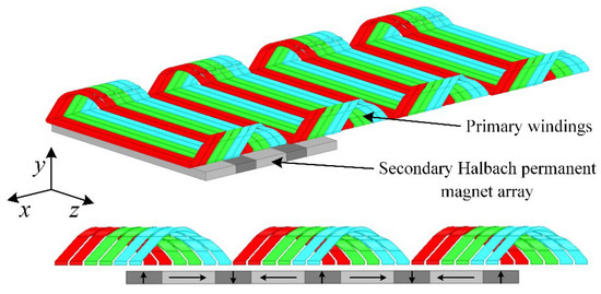
Figure 1.
Unilateral structure diagram of IHPMSLM.

Table 1.
Structure parameters of INPMSLM.
3. Magnetic Field Analysis and Finite Element Verification
3.1. Unilateral IHPMSLM Magnetic Field Resolution Model
Due to the unique structure of the IHPMSLM, the magnetic circuit is closed via the air gap. There are significant distortions in the excitation field at the side-end positions of the secondary permanent magnet array, so it is necessary to consider the side-end effects of the secondary field to accurately solve the air-gap magnetic field distribution and calculate the periodic steady-state electromagnetic thrust.
As shown in Figure 2, according to the finite element static field simulation results of the Halbach permanent magnet array, the whole array with length L in the x-direction can be divided into three parts, namely, the sinusoidal-like region and the edge-end distortion region, according to the actual distribution of the magnetic induction intensities Bxpm and Bypm at the position of line one in the air gap. If the pole pitch of the permanent magnet array is τ, the symmetry period of the air-gap magnetic density in the sine-like zone is still 2τ. Still, the air-gap magnetic density in the end distortion zone does not follow this symmetry law. Define ɛ as the distance from the edge of the permanent magnet array when the magnetic field decays to zero. Based on the results of the finite element static magnetic field simulation, it can be approximated as ɛ = τ; i.e., the magnetic fields do not affect each other when the distance between two adjacent permanent magnet arrays is 2ɛ. As shown in Figure 3, assuming that the permanent magnet array is infinitely long in the x-direction, the permanent magnet array after considering the edge-end effect will be symmetrically periodic, which is said to be a mechanical pseudo-period [11]; i.e., λ = L + 2τ.
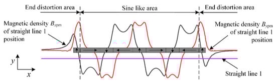
Figure 2.
Air-gap Magnetic Field Distribution of the Halbach Permanent Magnet Array.
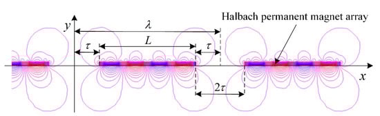
Figure 3.
Infinitely long Halbach permanent magnet array.
If we consider the influence of the IHPMSLM secondary permanent magnetic array edge effect, the mechanical pseudo-periodic constant λ can be used as the period of the modified Fourier series; that is, the end distortion area of the permanent magnet array itself plus the magnetic field is regarded, as a whole, as the period of integration of the magnetization strength M and no longer takes 2τ as the integration period. Magnetization intensity M is the line integrated over the range λ to obtain the spatial distribution of the magnetization intensity, thus solving for the air-gap magnetic field on the solid side of the Halbach permanent magnet array and accounting for the side-end effect with the help of the magnetic vector potential and boundary conditions. To establish an analytical model of the IHPMSLM air-gap magnetic field considering the secondary side-end effect, the Halbach permanent magnet array magnetic field and the primary six-phase winding magnetic field can be solved separately and then superimposed, and based on the bilateral symmetric structure of the IHPMSLM, only a single-sided air-gap magnetic field needs to be solved. Therefore, an analytical model of the single-sided IHPMSLM magnetic field with infinite length in the x-direction is established, as shown in Figure 4. Regions I, II, and III are the permanent magnet array region, the air-gap region on the weak magnetic side of the permanent magnet array, and the air-gap region on the solid magnetic side of the permanent magnet array, respectively, and are used for solving the secondary Halbach permanent magnet array air-gap magnetic field accounting for the edge-end effects. Regions IV, V, and VI are the primary six-phase winding region and the air-gap regions on both sides of the winding and are used for solving the primary winding air-gap magnetic field. In Figure 4, hm is the thickness of the permanent magnet array, hc is the thickness of the winding, and is the air-gap length.
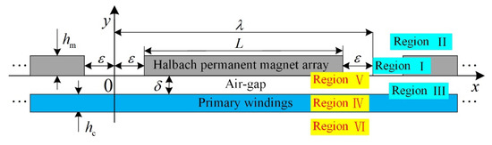
Figure 4.
Unilateral IHPMSLM magnetic field analysis model.
This paper separately solves the IHPMSLM primary and secondary air-gap magnetic fields using magnetic vector potential. To simplify the calculation, the basic assumptions are as follows: (1) There is no change in the magnetic field along the z-direction, and only the directional component of the primary winding current exists. (2) The IHPMSLM extends infinitely along the x-direction. (3) Each permanent magnet in the Halbach permanent magnet array is uniformly magnetized and non-demagnetized. The recovery curve coincides with the demagnetization curve, and the permeability is equal to the air permeability.
3.2. Halbach Permanent Magnet Array Magnetic Field Analysis and Element Verification
An analytical model of the magnetic field of the Halbach permanent magnet array with one mechanical pseudo-cycle is shown in Figure 5.
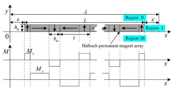
Figure 5.
Analytical model of the Halbach permanent magnet array magnetic field.
In Figure 5, bm is the width of the permanent magnet magnetized in the y-direction, and the pole arc factor αp of the Halbach permanent magnet array is bm/τ. The arrow indicates the direction of magnetization of the permanent magnet.
Based on the basic assumption (3), the spatial distribution function of the magnetization intensity of the Halbach permanent magnet array can be expressed as follows:
According to the principle of the Fourier series decomposition of square waves, the following equation can solve Mx and My in Figure 5:
where m1 = 2nπ/λ.
The following equation can calculate the Fourier coefficients an and bn:
In the above formula, Br is the remanent magnetization of the permanent magnet.
The equivalent magnetization current density of the Halbach permanent magnet array is
The two-dimensional constant electromagnetic field equation is
In addition, the introduction of vector magnetic potential A makes
Substituting Equation (5) into Equation (4), we obtain
Therefore, there are only z-directional components of A and J, so Equation (7) can be reduced to
Thus, the expressions for the magnetic induction strengths Bx and By are as follows:
The magnetic vector potential of region i (I = I, II, III) is assumed to be Ai (x, y), thus establishing the magnetic field equation for each region vector magnetic potential as shown in Equation (4) and obtaining the general solution of each region vector magnetic potential in the equation via the method of separating variables.
The regions in Figure 5 satisfy the following boundary conditions:
We bring the boundary conditions in Equation (11) into the vector magnetic potential general solution and obtaining the coefficients in the general solution. Afterward, insert the vector magnetic potential expression into Equation (9) to obtain the analytical equation of the Halbach permanent magnet array air-gap magnetic density in the region, considering the edge-end effect as follows:
To verify the correctness of the analytical result of Equation (12), a two-dimensional static magnetic field finite element simulation model of a finite-length Halbach permanent magnet array, as shown in Figure 2, is built in the software named ANSYS Electronics Desktop 2021 R1, and balloon boundary conditions are imposed. To obtain the magnetic density waveform at the position, we use in Figure 5, as shown in Figure 6.
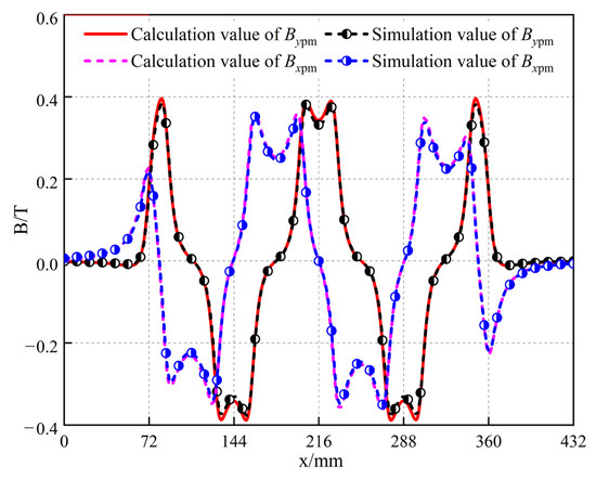
Figure 6.
Finite element verification of Halbach permanent magnet array air-gap magnetic density analysis results.
In Figure 6, the Bxpm and Bypm waveforms obtained by the analytical and finite element methods agree. The error between the simulated and calculated values at each position in the curve as a proportion of the amplitude of the waveform obtained from the simulation was used to measure the maximum error. The maximum errors are 4.28% and 5.15% of the amplitudes obtained from the simulation, respectively. The analyzed values of the air-gap magnetic density are slightly more prominent because the results of the analytical method based on ideal assumptions are more idealized.
A comparison of the calculated air-gap magnetic field values, Bxpm and Bypm, of the Halbach permanent magnet array when the edge-end effect is considered and the calculated air-gap magnetic field values, Bxn and Byn, of the Halbach permanent magnet array when the edge-end effect is not considered is shown in Figure 7.
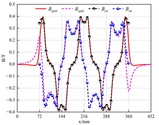
Figure 7.
Comparison of magnetic field edge-end effects.
The results show that the Halbach permanent magnet array magnetic field solution method based on a mechanical pseudo-period can accurately portray the actual distribution of the air-gap magnetic field, thus laying the theoretical foundation for the accurate solution of the electromagnetic thrust and normal electromagnetic force.
3.3. Primary Winding Magnetic Field Analysis and Finite Element Verification
The analytical model of the magnetic field of the primary six-phase winding is shown in Figure 8.
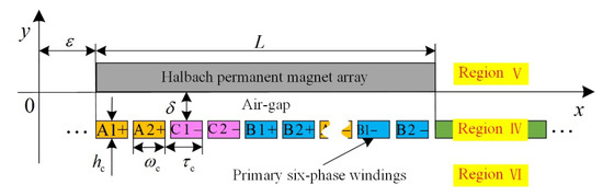
Figure 8.
Analytical model of primary winding magnetic field.
Define the single primary winding pseudo-pole arc factor as αc = ωc/τc, where ωc is the width of the single winding, and τc is the width of the space occupied by the single winding.
The single-sided IHPMSLM primary six-phase semi-symmetric winding current expression is as follows:
In Formula (13), Im is the primary current amplitude, and θ0 is the initial phase angle of the primary current.
Since the expressions of the current and electric density of each phase winding are similar, only the difference in phase sequence exists; therefore, only the A1 phase winding current density needs to be solved by shifting the A1 phase winding current density τc to obtain the Fourier series expansion of the remaining phase winding current density.
The expression for the current density of the A1 phase winding is as follows:
If kπ/τc = 6 m2, then the Fourier series expansion of the A1 phase winding current density in the coordinate system in Figure 8 is as follows:
Therefore, the Fourier series expansion of the primary six-phase winding current density is
Similarly to the analytical process of the Halbach permanent magnet array air-gap magnetic field, the magnetic vector potential of region j (j = IV, V, VI) is assumed to be Aj (x, y) by establishing the magnetic field equations of the magnetic vector potential in three regions and using the variable separation method to obtain the general solution of each magnetic vector potential in the system shown in Equation (16).
The winding and air-gap areas in Figure 8 satisfy the following boundary conditions:
Bringing the boundary condition in Equation (18) into the vector magnetic potential flux solution and obtaining the expression of the magnetic vector potential Aj (x, y) to obtain the expression of the radial air-gap magnetic density of the A1 phase winding by shifting the phase, the radial air-gap magnetic density of the remaining phases is obtained, and finally, using the superposition principle, the air-gap magnetic density of the primary six-phase winding is solved:
To verify the correctness of (19), a single-sided IHPMSLM primary six-phase winding finite element two-dimensional transient field simulation model in ANSYS, with the winding excitation as shown in Formula (13) added to it, is applied to calculate the primary six-phase winding air-gap magnetic field distribution under load conditions, and this calculation is compared with the calculated results. Figure 9 shows the winding air-gap magnetic density at the initial moment under the three pairs of poles in the same position between the calculation model and the simulation model.
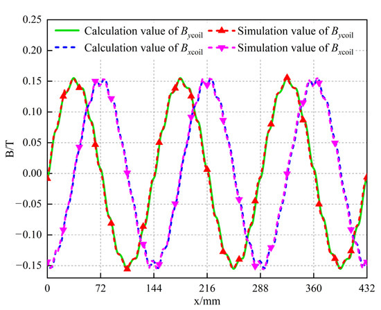
Figure 9.
Finite element verification of magnetic field analysis results of primary six-phase winding air gap.
The results show that the six-phase winding air-gap magnetic density of the Bxcoil and Bycoil waveforms obtained by the analytical and finite element methods in Figure 9 are in good agreement. Similarly, the maximum value of the error between the analyzed and simulated values at all positions as a proportion of the amplitude obtained from the simulation is called the maximum error. The maximum errors are 5.614% and 4.604% of the amplitudes obtained from the simulation, respectively, which verifies the correctness of the analytical results of the magnetic field of the primary winding.
3.4. Air-Gap Synthesis Magnetic Field Analysis and Finite Element Verification
By overlaying the radial and tangential components of the secondary permanent magnet array air-gap magnetic density and the primary winding magnetic density, the IHPMSLM air-gap composite magnetic density expression is
We added the excitation of the primary winding in Formula (13) to the simulation model of the transient field with a single-sided IHPMSLM and set the secondary motion’s velocity to 0 m/s. The analyzed and simulated values of the synthetic magnetic density are set at the center line of the air gap, considering the effect of the secondary side as shown in Figure 10, at the initial moment under the three pairs of poles in the same position between the calculation model and the simulation model.
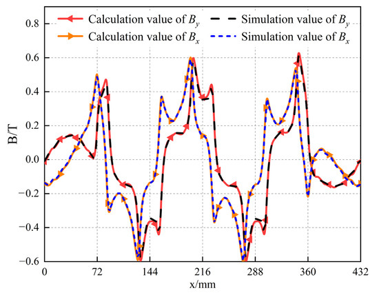
Figure 10.
Finite element verification of analytical results of air-gap synthesis magnetic field.
At any moment within a current cycle, the error between the analyzed and simulated values of the air-gap synthetic magnetic density is about 5%, which satisfies the need for engineering analysis and verifies the correctness of the theoretical derivation.
4. Electromagnetic Force Modeling and Optimization
4.1. Electromagnetic Force Calculation
Since the primary and secondary phases of the IHPMSLM are bilaterally symmetrical, we can only calculate one side of the electromagnetic force. The effect of the secondary side end effect is included in the Formula (12) of the resolved magnetic field of the permanent magnet array; therefore, the electromagnetic thrust Fx and the normal electromagnetic force Fy of the single-sided IHPMSLM at each moment when the secondary is running at the synchronous speed vs based on the result of the magnetic field analysis of the load air-gap calculation can be used using the Maxwell tensor method.
The Maxwell tensor method equates the mass force f in a magnetic field to a set of tensors and expresses it using the stress tensor T as
where V is the volume subregion enclosing the computational object, and S is the surface enclosing the V region.
For the plane-parallel electromagnetic field in this study, the surface integral can be further simplified to a curve integral, from which we can calculate the Fx and Fy of the IHPMSLM secondary permanent magnet array at a particular moment, respectively, as follows:
where l is the closed curve abcda enclosing the secondary permanent magnet array in Figure 11, w is the length of the z-direction of IHPMSLM, and nx, ny are the unit standard vector x and y plane components of dl, respectively.
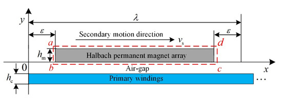
Figure 11.
Single-sided IHPMSLM electromagnetic thrust calculation model.
4.2. Finite Element Verification of Electromagnetic Force Calculation Results
We apply the excitation as formula (13) to the primary winding in the single-sided IHPMSLM finite element transient field simulation model and add a force matrix to the secondary permanent magnet array, which is set to move uniformly and linearly at a synchronous speed and along the positive axis direction. Then, we calculate Fx and Fy on the single-sided IHPMSLM secondary during the running time.
The calculated results of the single-sided IHPMSLM secondary electromagnetic force under the periodical steady-state operation condition obtained from the analytical calculation are compared with the finite element simulation results, Fx is shown in Figure 12a and Fy is shown in Figure 12b.
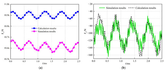
Figure 12.
Electromagnetic force verification.
The average values of unilateral electromagnetic thrust Fxavg obtained by the analytical method and the finite element method in Figure 12a are 10.901 kN and 10.623 kN, respectively, and there is a calculation error of 278 N between them, which accounts for about 2.55% of the average thrust obtained by the analytical method. The analytical result is significant because the Maxwell tensor method calculates the electromagnetic thrust directly by the air-gap magnetic field, and the calculation result of the air-gap magnetic field based on the ideal assumptions is slightly larger than the simulation value. The reason is that the Maxwell tensor method calculates the electromagnetic thrust directly from the air-gap magnetic field, and the calculation result of the air-gap magnetic field based on ideal assumptions is slightly larger than the simulated value, which leads to a sizeable analytical result of the electromagnetic force compared with the simulated value. Meanwhile, the peak values of unilateral electromagnetic thrust Fxpk obtained by the analytical method and the finite element method are 70.472 N and 87.356 N, respectively, and the errors of both are relatively small.
Since the IHPMSLM does not have a core, its unilateral normal electromagnetic force Fy is small. As shown in Figure 12b, the waveform trends obtained by the analytical method and the finite element method match, and the average values are −115.646 N and −105.084 N, respectively, which is about 9.13% of the average value obtained by the analytical method. The reason is that the current density in the winding area is equivalent to the wire density at the center of the winding in the analytical calculation, thus ignoring the effect of the skin effect of the conductor under high current excitation, which leads to extensive analytical results. However, the bilateral symmetric structure of the IHPMSLM will cancel Fy, making the overall normal electromagnetic force in the motor secondary zero.
From Formula (23), the load air-gap magnetic field will directly affect the electromagnetic thrust, impacting Fxavg and Fxpk. Therefore, optimizing the key structural parameters of the IHPMSLM is necessary to enhance Fxavg without increasing Fxpk, thus further increasing the power density.
4.3. Electromagnetic Thrust Optimization
The parameters αp, hm, hc, ωc, and are the critical variables of the IHPMSLM-loaded air-gap magnetic field. Due to the long stroke of the IHPMSLM in this study and the absence of core parts, the primary winding is only supported by the stator skeleton to avoid mechanical friction between moving parts and stationary parts due to force deformation during the non-periodic transient operation of the motor, the mechanical air-gap is still selected to be ẟ = 5 mm constant. Therefore, the parameters αp, hm, hc, and ωc can be used as optimization variables to find the optimal combination of optimization variables, which makes the calculated value of Fxpk not increase and places the maximum calculated value of Fxavg under the constraint that the thickness of theunilateral IHPMSLM is constant, i.e., hm + hc + = 20 mm, using a GA to obtain the best solution for the optimal design of the IHPMSLM. The optimization objective functions are as follows:
Considering the motor design, processing and assembly, and winding casting and molding, we can select the constraint range of optimization variables in Table 2 to make the optimization results more reasonable.
Table 2.
Optimizing the range of variable constraints.
To clarify the parameter sensitivity order and its contribution degree to the resounding optimization results and to determine the critical optimization variables, the correlation matrix of optimization variables in Figure 13 was calculated using a GA. The positive and negative signs of the elements in the figure represent positive and negative correlations, respectively, and the magnitude of the element values directly reflects the strength of the correlation between the parameters.
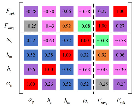
Figure 13.
Parameter correlation matrix.
Overall, the four optimization variables are all related to Fxavg and Fxpk to different degrees, among which only variable hm shows a strong positive correlation with Fxavg; i.e., an increase in the volume of permanent magnets will significantly increase the average thrust. In contrast, variable ωc shows a relatively strong negative correlation with Fxpk; i.e., a reasonable choice of winding width can effectively reduce the peak value of thrust fluctuation. Variables αp, and hc can reduce the peak value of thrust fluctuation while decreasing the average thrust. In addition, the interaction between optimization variables is more significant. Hence, optimizing a single variable often fails to meet the performance requirements. So, finding the optimal combination of optimization variables to meet the optimization objectives is the key to electromagnetic force optimization.
To further verify the parameter sensitivity analysis’s conclusions, draw the optimized variables’ response surfaces as shown in Figure 14 and Figure 15. Where Figure 14a,b show the response surface of the average thrust and Figure 15a,b show the response surfaces of peak to peak thrust fluctuations. The change in the value of αp can significantly affect Fxavg and reaches its maximum around 0.5, while Fxpk fluctuates more with the increase in the value of αp. At the same time, the increase in the value of hm causes a smaller change in Fxpk, but a more significant lift in Fxavg. In addition, the increase in the value of ωc can significantly reduce Fxpk and make Fxavg constant. Finally, Fxavg and Fxpk all decrease significantly with the increase in the value of hc. Therefore, we need to weigh the pros and cons of choosing parameters during optimization.
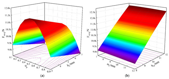
Figure 14.
Response surface of average thrust.
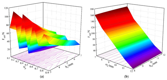
Figure 15.
Response surface of thrust fluctuation peak to peak.
The computational flow chart of the GA is shown in Figure 16.
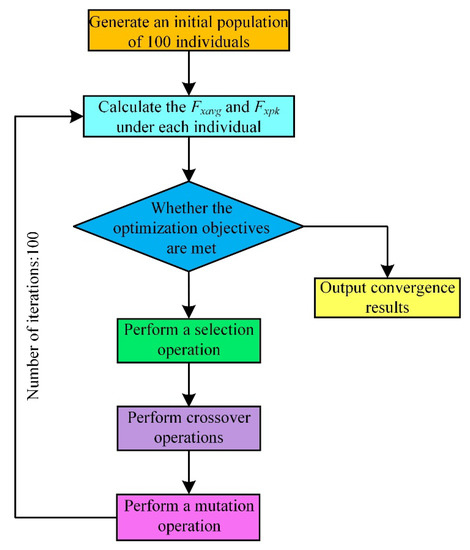
Figure 16.
GA flow chart.
A set of Pareto optimal solution sets satisfying the optimization objective is finally obtained by calculation, as shown in Table 3.
Table 3.
Optimal combination of optimization variables.
To verify the correctness of the above optimal combination of optimization variables, establish a one-sided IHPMSLM finite-element two-dimensional transient field parametric simulation model that uses the optimal combination of optimization variables in Table 3 as input to obtain the Fx optimization results shown in Figure 17.
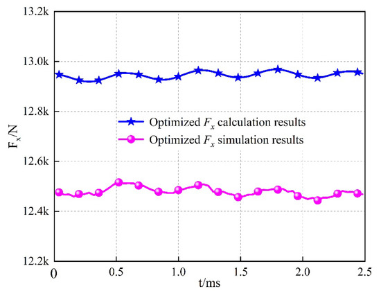
Figure 17.
Optimized electromagnetic thrust curve.
The optimization results are shown in Table 4 when compared to the pre-optimization Fx waveform in Figure 12.
Table 4.
Electromagnetic thrust optimization results.
As can be seen from Table 4, the optimized Fxavg calculated value is 18.75% higher, and the Fxpk calculated value is 30.27% lower, than before optimization, while the optimized Fxavg simulated value is 17.46% higher, and the Fxpk simulated value is 28.76% lower, than before optimization. The calculated results are in good agreement with the simulation results. In addition, the optimized unilateral IHPMSLM average thrust is improved significantly, and the thrust fluctuation is reduced significantly, which initially achieves the optimization goal and verifies the application of the GA and the correctness of the optimization results.
The good electromagnetic performance of the optimized IHPMSLM comes at the expense of its economic cost. The increase in hm leads to an 18% increase in permanent magnet usage, thus increasing the economic cost; however, reducing hc will reduce copper usage by 25.76%. Therefore, the optimal combination of variables can be used as a reference for the optimized design of the IHPMSLM, making it more suitable for high-power-density applications.
5. Conclusions
To solve the electromagnetic force optimization problem of the IHPMSLM, this paper adopts an optimization method based on the combination of analytical calculation and a genetic algorithm, which is fast and can greatly save calculation time. The specific conclusions are as follows:
- (1)
- A single-sided IHPMSLM magnetic field analytical model that can simultaneously solve the primary and secondary air-gap magnetic fields has been established, in which the secondary Halbach permanent magnet array magnetic field is solved by combining the pseudo-periodic idea with the equivalent magnetization strength method, which is less computationally intensive and accurately depicts the air-gap magnetic field in the sinusoidal-like region and the end aberration region of the permanent magnet array. Additionally, the primary six-phase winding magnetic field is solved using the Fourier series expansion method. By superposing the primary and secondary air-gap magnetic fields, the synthetic magnetic field of the IHPMSLM air gap is obtained, which fits the actual distribution of the magnetic field, and the error meets the needs of engineering analysis and matches well with the finite element results, which solves the problem of accurately solving the air-gap magnetic field of the IHPMSLM load.
- (2)
- Based on the solution results of the air-gap magnetic field, the Maxwell tensor method is used to establish the functional relationship between the tangential electromagnetic thrust and the normal electromagnetic force of the unilateral IHPMSLM and the main structural parameters of the motor, and the correctness of the electromagnetic force modeling is verified by the finite element, which provides the theoretical q for the calculation of the motor performance.
- (3)
- Taking the Halbach permanent magnet array and the main structural parameters of the primary winding as the optimization variables, based on the parameter sensitivity analysis and response surface calculation, within the constraints of the values of the optimization variables, the genetic algorithm is used to search for the Pareto optimal solution set of the optimization objective, and the computational results show that the average thrust of the unilateral IHPMSLM following the optimization is increased by 18.75%, the peak-to-peak thrust fluctuation is decreased by 30.27%, and the error is small compared with the finite element results. The decrease of 30.27% and the error with the finite element results are small, which verifies the reasonableness of the optimization method, and the optimization results can be used as a reference for the optimal design of IHPMSLM.
Author Contributions
Conceptualization, Z.S.; supervision Z.S. and C.H.; methodology, G.J.; validation, W.Z. and Y.M.; investigation, G.J.; data curation, G.J. and Z.L.; writing—original draft preparation, G.J.; writing—review and editing, Z.S.; project administration, C.H.; funding acquisition, C.H.; formal analysis, W.Z.; software, W.Z. and Y.M. All authors have read and agreed to the published version of the manuscript.
Funding
This research was funded by the National Natural Science Foundation of China, grant number 52077218.
Conflicts of Interest
The authors declare no conflict of interest.
References
- Yu, L.; Chang, S.; He, J.; Sun, H.; Huang, J.; Tian, H. Electromagnetic Design and Analysis of Permanent Magnet Linear Synchronous Motor. Energies 2022, 15, 5441. [Google Scholar] [CrossRef]
- Zhou, W.; Sun, Z.; Cui, F.; Mao, Y. Electromagnetic Design of High-Speed and High-Thrust Cross-Shaped Linear Induction Motor. IEEE Access 2021, 9, 87501–87509. [Google Scholar] [CrossRef]
- Zhang, Z.; Luo, M.; Duan, J.-A.; Kou, B. Design and Modeling of a Novel Permanent Magnet Width Modulation Secondary for Permanent Magnet Linear Synchronous Motor. IEEE Trans. Ind. Electron. 2022, 69, 2749–2758. [Google Scholar] [CrossRef]
- Choi, J.-S.; Yoo, J. Design of a Halbach Magnet Array Based on Optimization Techniques. IEEE Trans. Magn. 2008, 44, 2361–2366. [Google Scholar] [CrossRef]
- Wei, W.; Zhang, J.; Yao, J.; Tang, S.; Zhang, S. Performance Analysis and Optimization of Power Density Enhanced PMSM with Magnetic Stripe on Rotor. Energies 2020, 13, 4457. [Google Scholar] [CrossRef]
- Liu, X.; Zheng, X.; Wang, X. Modeling of Uneven Air Gap Magnetic Field for Disc Planetary Permanent Magnet Machine with Segmented Gap Halbach Array. IEEE Trans. Energy Convers. 2023, 38, 693–702. [Google Scholar] [CrossRef]
- Li, B.; Zhang, J.; Zhao, X.; Liu, B.; Dong, H. Research on Air Gap Magnetic Field Characteristics of Trapezoidal Halbach Permanent Magnet Linear Synchronous Motor Based on Improved Equivalent Surface Current Method. Energies 2023, 16, 793. [Google Scholar] [CrossRef]
- Zhang, X.; Zhang, C.; Yu, J.; Du, P.; Li, L. Analytical Model of Magnetic Field of a Permanent Magnet Synchronous Motor with a Trapezoidal Halbach Permanent Magnet Array. IEEE Trans. Magn. 2019, 55, 8105205. [Google Scholar] [CrossRef]
- Ladghem-Chikouche, B.; Boughrara, K.; Dubas, F.; Ibtiouen, R. 2-D Semi-Analytical Magnetic Field Calculation for Flat Permanent-Magnet Linear Machines Using Exact Subdomain Technique. IEEE Trans. Magn. 2021, 57, 8106211. [Google Scholar] [CrossRef]
- Cao, D.; Zhao, W.; Ji, J.; Wang, Y. Parametric Equivalent Magnetic Network Modeling Approach for Multiobjective Optimization of PM Machine. IEEE Trans. Ind. Electron. 2021, 68, 6619–6629. [Google Scholar] [CrossRef]
- Du, Y.; Huang, Y.; Guo, B.; Peng, F.; Dong, J. Semianalytical Model of Multiphase Halbach Array Axial Flux Permanent-Magnet Motor Considering Magnetic Saturation. IEEE Trans. Transp. Electrif. 2023, 9, 2891–2901. [Google Scholar] [CrossRef]
- Li, H.; Li, T. End-Effect Magnetic Field Analysis of the Halbach Array Permanent Magnet Spherical Motor. IEEE Trans. Magn. 2018, 54, 8202209. [Google Scholar] [CrossRef]
- Guo, L.; Zhou, Q.; Galea, M.; Lu, W. Cogging Force Optimization of Double-Sided Tubular Linear Machine with Tooth-Cutting. IEEE Trans. Ind. Electron. 2022, 69, 7161–7169. [Google Scholar] [CrossRef]
- Li, Z.; Xia, J.; Guo, Z.; Lu, B.; Ma, G. Reduction of Pole-Frequency Vibration of Surface-Mounted Permanent Magnet Synchronous Machines with Piecewise Stagger Trapezoidal Poles. IEEE Trans. Transp. Electrif. 2023, 9, 833–844. [Google Scholar] [CrossRef]
- Dreishing, F.; Kreischer, C. Optimization of Force-to-Weight Ratio of Ironless Tubular Linear Motors Using an Analytical Field Calculation Approach. IEEE Trans. Magn. 2022, 58, 7401704. [Google Scholar] [CrossRef]
- Zhao, Y.; Li, Y.; Lu, Q. An Accurate No-Load Analytical Model of Flat Linear Permanent Magnet Synchronous Machine Accounting for End Effects. IEEE Trans. Magn. 2023, 59, 8100111. [Google Scholar] [CrossRef]
- Kim, K.-H.; Cho, H.-K.; Woo, D.-K. 3D Characteristic Analysis of 3-Leg Linear Permanent Magnet Motor with Magnet Skew and Overhang Structure. IEEE Access 2021, 9, 153863–153874. [Google Scholar] [CrossRef]
- Song, Z.; Liu, C.; Feng, K.; Zhao, H.; Yu, J. Field Prediction and Validation of a Slotless Segmented-Halbach Permanent Magnet Synchronous Machine for More Electric Aircraft. IEEE Trans. Transp. Electrif. 2020, 6, 1577–1591. [Google Scholar] [CrossRef]
- Zhao, J.; Mou, Q.; Guo, K.; Liu, X.; Li, J.; Guo, Y. Reduction of the Detent Force in a Flux-Switching Permanent Magnet Linear Motor. IEEE Trans. Energy Convers. 2019, 34, 1695–1705. [Google Scholar] [CrossRef]
- Chi, S.; Yan, J.; Shan, L.; Wang, P. Detent Force Minimizing for Moving-Magnet-Type Linear Synchronous Motor. IEEE Trans. Magn. 2019, 55, 8102005. [Google Scholar] [CrossRef]
- Chung, S.-U.; Lee, J.-Y. Teeth Arrangement and Pole–Slot Combination Design for PMLSM Detent Force Reduction. Energies 2021, 14, 8141. [Google Scholar] [CrossRef]
- Cervone, A.; Slunjski, M.; Levi, E.; Brando, G. Optimal Third-Harmonic Current Injection for Asymmetrical Multiphase Permanent Magnet Synchronous Machines. IEEE Trans. Ind. Electron. 2021, 68, 2772–2783. [Google Scholar] [CrossRef]
- Huang, C.; Kou, B.; Zhao, X.; Niu, X.; Zhang, L. Multi-Objective Optimization Design of a Stator Coreless Multidisc Axial Flux Permanent Magnet Motor. Energies 2022, 15, 4810. [Google Scholar] [CrossRef]
- Grenier, J.-M.; Pérez, R.; Picard, M.; Cros, J. Magnetic FEA Direct Optimization of High-Power Density, Halbach Array Permanent Magnet Electric Motors. Energies 2021, 14, 5939. [Google Scholar] [CrossRef]
- Zhao, W.; Ma, A.; Ji, J.; Chen, X.; Yao, T. Multiobjective Optimization of a Double-Side Linear Vernier PM Motor Using Response Surface Method and Differential Evolution. IEEE Trans. Ind. Electron. 2020, 67, 80–90. [Google Scholar] [CrossRef]


Disclaimer/Publisher’s Note: The statements, opinions and data contained in all publications are solely those of the individual author(s) and contributor(s) and not of MDPI and/or the editor(s). MDPI and/or the editor(s) disclaim responsibility for any injury to people or property resulting from any ideas, methods, instructions or products referred to in the content. |
© 2023 by the authors. Licensee MDPI, Basel, Switzerland. This article is an open access article distributed under the terms and conditions of the Creative Commons Attribution (CC BY) license (https://creativecommons.org/licenses/by/4.0/).