Article

Performance Analysis of Solar Tracking Systems by Five-Position Angles with a Single Axis and Dual Axis

by
Nuttee Thungsuk
1,
Thaweesak Tanaram
2,
Arckarakit Chaithanakulwat
1,
Teerawut Savangboon
1,
Apidat Songruk
3,
Narong Mungkung
3,
Theerapong Maneepen
4,
Somchai Arunrungrusmi
3,*,
Wittawat Poonthong
5,
Nat Kasayapanand
5,*,
Siriwhut Nilwhut
6,
Hiroyuki Kinoshita
7 and
Toshifumi Yuji
8
1
Electrical Engineering, Dhonburi Rajabhat University Samut-Prakan, Samut-Prakan 10540, Thailand
2
Faculty of Industrial Technology, Pibulsongkram Rajabhat University, Phitsanulok 65000, Thailand
3
Department of Electrical Technology Education, King Mongkut’s University of Technology, 126 Pracha Uthit Rd., Bang Mot, Thung Khru, Bangkok 10140, Thailand
4
Department of Production Technology Education, King Mongkut’s University of Technology, 126 Pracha Uthit Rd., Bang Mot, Thung Khru, Bangkok 10140, Thailand
5
Energy Technology Program, School of Energy, Environment and Materials, King Mongkut’s University of Technology Thonburi, 126 Pracha Uthit Rd., Bang Mod, Thung Khru, Bangkok 10140, Thailand
6
Faculty of Industrial Technology, Nakhon Phanom University, Nakhon Phanom 48000, Thailand
7
Mechanical Design Systems Engineering, Faculty of Engineering, University of Miyazaki, 1-1, Gakuenkibanadai-nishi, Miyazaki 889192, Japan
8
Faculty of Education, University of Miyazaki, 1-1, Gakuenkibanadai-nishi, Miyazaki 889192, Japan
*
Authors to whom correspondence should be addressed.
Energies 2023, 16(16), 5869; https://doi.org/10.3390/en16165869
Submission received: 23 February 2023 / Revised: 22 June 2023 / Accepted: 3 July 2023 / Published: 8 August 2023
(This article belongs to the Section A2: Solar Energy and Photovoltaic Systems)

Abstract

:
This research presents an analysis of the five-position angle in both single-axis (one-axis tracking) and dual-axis (two-axis tracking) solar tracking systems. The study compares these tracking systems, where four solar panels move simultaneously, with a fixed solar panel system. The findings revealed that the five-position angle Sun-tracking technique resulted in lower energy consumption by the tracking mechanism than in the case of an all-time solar tracking system. The key component of the implemented system is a light-dependent resistor (LDR) sensor for controlling the motion of the motor for five positions on the vertical axis and horizontal axis, processed by a microcontroller to ensure the necessary solar tracking always moves in a perpendicular direction. According to the results, the voltage, current, and power increased with both one-axis and two-axis tracking compared to those of the fixed solar panel system under the same conditions. However, when evaluating the total energy with numerical integration methods, one-axis and two-axis provided 183.12 Wh and 199.79 Wh, respectively. Consequently, the energy production of the one-axis tracking system and the one-axis tracking system was found to be 16.71% and 24.97%, respectively, when compared to the fixed-axis system. Thus, the five-position angles of the sun-tracking technique resulted in lower energy consumption than is the case of an all-time solar tracking system.

1. Introduction

A solar cell is a device designed to directly convert light energy into electrical energy, making it highly suitable for the production of electricity. A standalone solar system is also well-suited for areas that are not connected to a power grid [1,2,3,4]. Furthermore, a solar farm exists for the purpose of generating electricity to be supplied to a power grid system. Solar power plants must incorporate appropriate designs of components such as inverters and transformers to effectively reduce costs and minimize energy losses [5]. However, it has been reported that maximum conversion efficiency requires direct sunlight perpendicular to the solar panel [6,7,8]. Most solar panel installations in Thailand currently use a fixed mounting system at an approximate angle of 15 degrees from the ground’s surface. Since the direction of sunlight is not always perpendicular to the solar panel [9], it is not possible to generate electrical energy throughout the day at full capacity. Therefore, a solar cell that can move to an alternative position according to that of the Sun is preferable since it can produce electricity efficiently all day long. Thus, a solar tracking system with a single axis [10,11,12,13] is widely used.
Many researchers have attempted to develop and invent a dual-axis solar tracking system using different technologies like mobile solar cell panels, which can track the position of the Sun based on calculations in each period of the year, or employing a control system with linear IC devices. Both systems have different advantages and disadvantages. The system controlled by a computer is expensive and needs to operate continuously all day, resulting in damage. The system with linear IC is more cost-effective but less efficient and flexible. Moreover, it responds to the system very slowly. According to the literature, microcontrollers are considered to be more flexible [4]. They are also accurate and reliable when used for long periods. Many manufacturers develop microcontrollers such as Atmel, Microchip, etc. [14,15,16].
One way of increasing the production of electrical energy is to use solar tracking that can operate in a perpendicular direction. Such a solar tracking system can have one axis or two axes. However, since a solar tracking system operates continuously, energy loss occurs in the motor drive and may be higher than the energy generated. In addition, the Sun’s solar radiation angle constantly changes throughout the day in different areas, and this is a factor to consider. Therefore, it is better for the propulsion system to use limited energy to follow the direction of sunlight from a solar tracking system in five-position angles. Using a microcontroller to control the solar tracking position with detection from an LDR sensor results in a simple and low-cost system. In this research, the study and analysis of the five-position angles of a solar tracking system involve a comparison of the one-axis (one-axis tracking) and dual-axis (two-axis tracking) solar tracking systems and the fixed solar panel system.

2. Theory of Solar Radiation

In the past, many people believed that if an area is sunny and hot, then it must have high potential for generating electricity from solar cells. However, an essential element to consider when installing solar panels to generate electricity is the radiant flux received by a surface per unit area (irradiance, I). The installation area is directly related to the generation of electricity. Light from the Sun is produced by a thermonuclear reaction, or a nuclear fusion reaction in the sun, becoming a source of energy and radiating to Earth. Figure 1 and Figure 2 show the geometric relationship between the plane of the Earth at any time of day and the direct rays of the Sun’s position relative to the plane.
Solar energy flux per unit area:
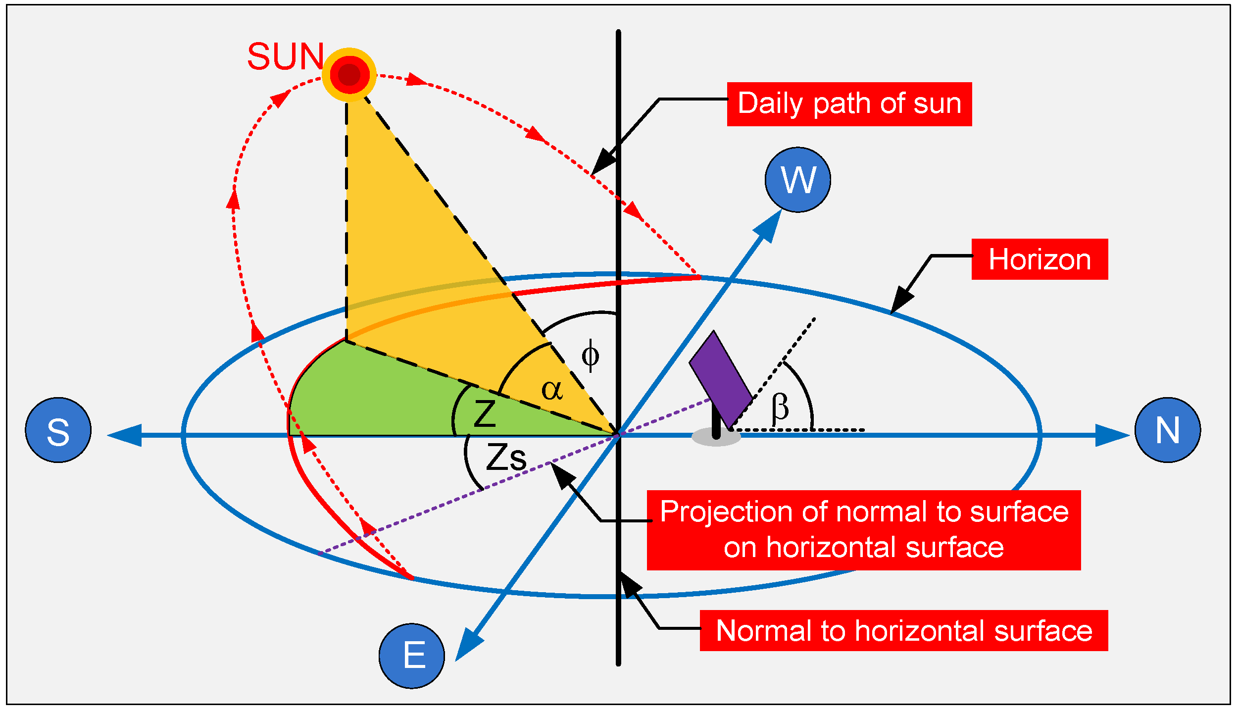
  • Latitude (L) is the angle north or south of the equator when measured to the north; positive and negative when measured to the south, ranging from −90 to 90 degrees;
  • The hour angle (h) represents the position of the Sun from the local meridian to the east or west. It is negative before the solar-noon period and positive after the solar-noon period, with a value of 15 degrees per hour;
  • The declination angle ( δ ) is the angle between the Sun’s rays in the solar-noon period and the equatorial plane. It is assigned a positive value when measuring north and a negative value when measuring south. The declination angle changes daily between −23.45 and 23.45 degrees. It can be calculated from Equation (1) [17].
    δ = 23.45   s i n 360 ( 284 + N ) 365
  • The solar altitude angle (a) is the angle between the Earth’s plane and the direct solar rays. The solar zenith angle (F) is the angle between natural and vertical solar radiation, as shown in Equation (2) [17].
    sin α = cos Φ = sin L sin α + c o s ( L ) cos δ cos h
  • The surface azimuth angle (Zs) is the angle between the south and the facing direction of the solar panel. It ranges from −180 to 180 degrees, and is zero, positive, or negative when the direction of the solar panel faces south, west, and east, respectively. Furthermore, b refers to the surface tilt angle from the horizontal plane.
  • The solar azimuth angle (Z) is the angle between the Sun’s vertical plane and the local meridian plane. The solar azimuth angle ranges from −180 to 180 degrees. The reference of the solar azimuth angle at the south (true south) is zero, while the south-to-west and south-to-east are positive and negative, respectively. It can be given as Equation (3) [17].
    sin Z = cos δ sin h cos α

3. Design and Experimental Setup

The technique presented in this study uses five-position control and four-panel tracking together with a one-axis and two-axis solar panel control tracking system. This technology differs from that used by other researchers, as detailed in Table 1. The design is divided into two parts: the structure and control system of solar panel tracking [18]. The details are as follows:
I.
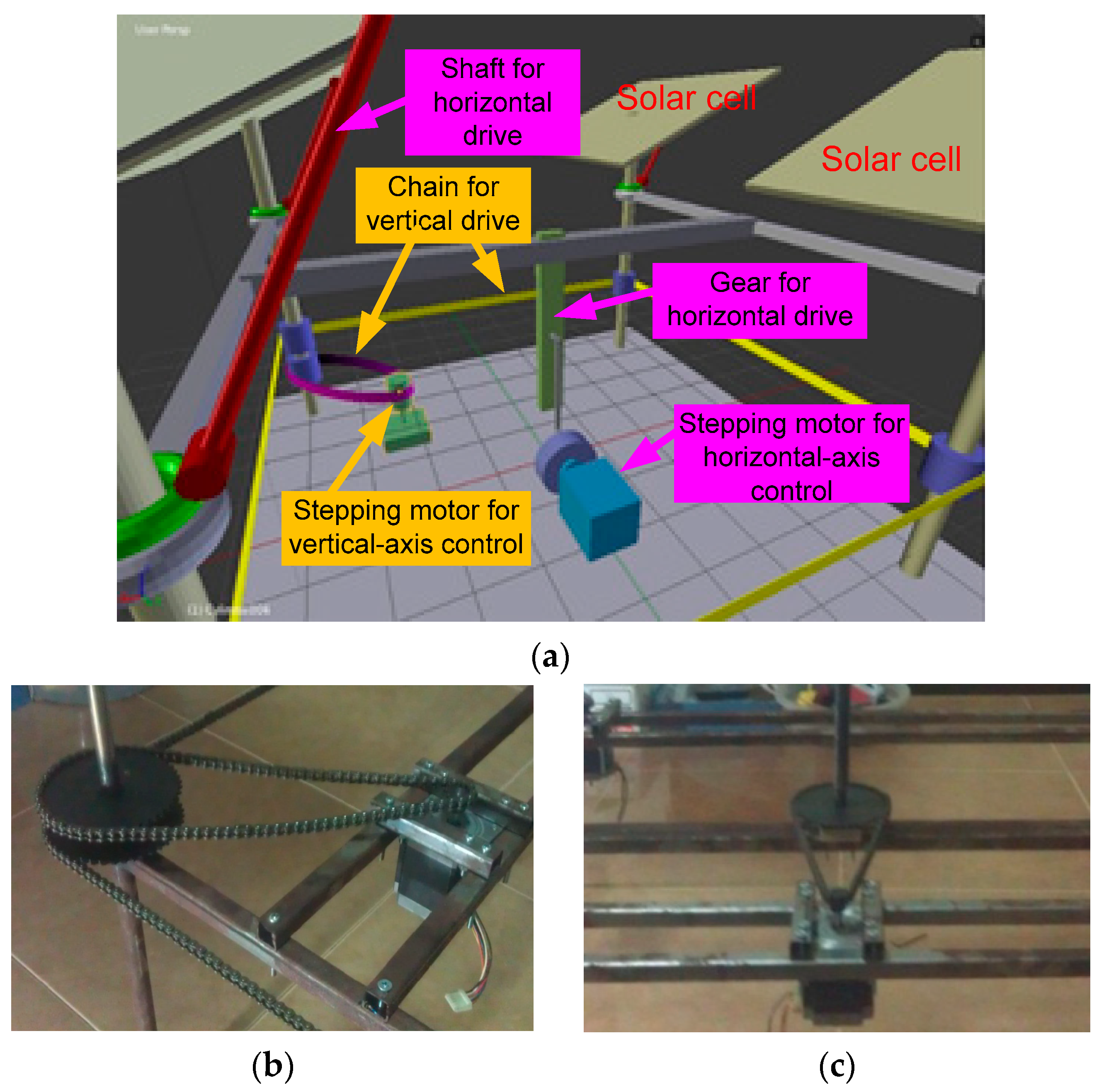
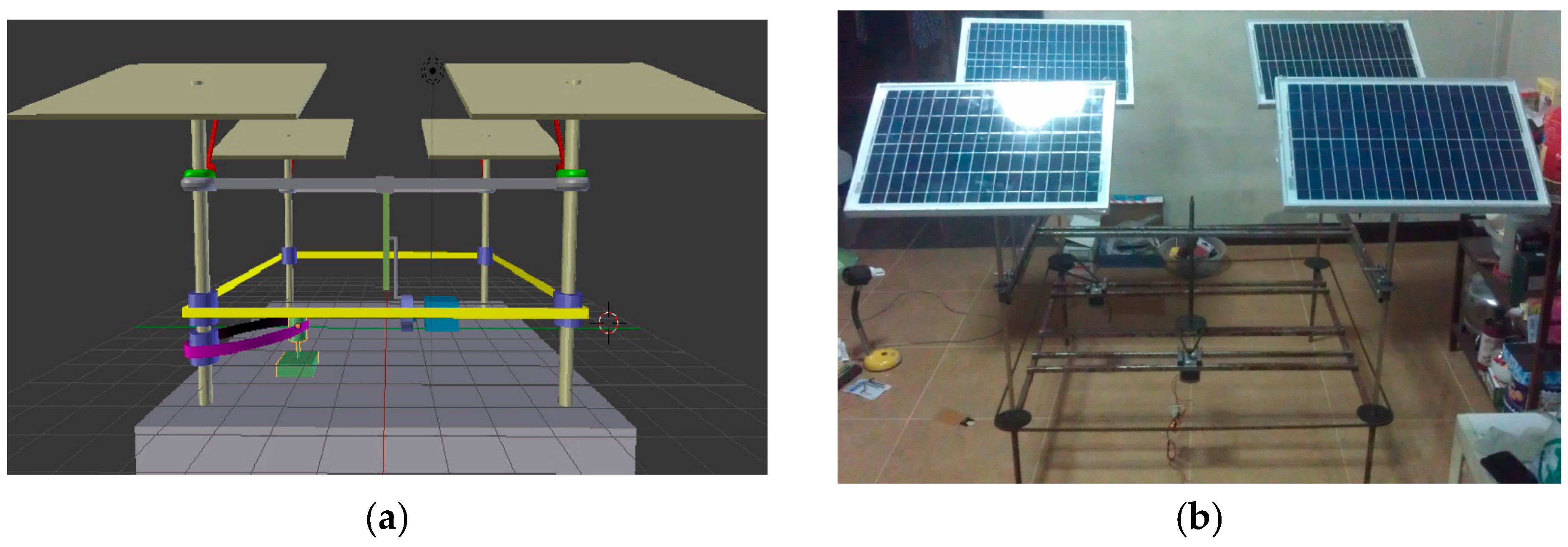
The structural design comprises four 10 W solar panels and two stepping motors, model syn 103h7124-1011, installed vertically and horizontally to drive the four solar panels moving together, as shown in Figure 3. All four solar panels are moved simultaneously using a chain and gear drive system for both vertical and horizontal axis movement, described as follows [11,22,23]:
  • Vertical axis movement uses the stepping motor (green motor in Figure 3a) to drive and transmit power through purple chains and the blue gear. The four rods with solar panels are installed on top, and the blue gears are wrapped around them with yellow chains. When the stepping motor is running, the purple chain mounted on the stepping motor drives the four blue gears mounted on each rod, with the four rods moving simultaneously, as shown in Figure 4.
  • Horizontal axis movement uses the stepping motor (blue motor in Figure 3a) to drive the crankshaft system which in turn drives the gray beams for the up-and-down movement of the solar panel. The red shaft is installed with solar panels and a ball-rolling rod. When the gray beams are raised, the red shafts move at a different angle, resulting in the solar panels tilting along the horizontal axis, as shown in Figure 4.
Figure 4. Equipment installed on the five-position angles of the axis solar panel tracking system. (a) Three-dimensional program; (b) vertical drive; (c) horizontal drive.
Energies 16 05869 g004
II.
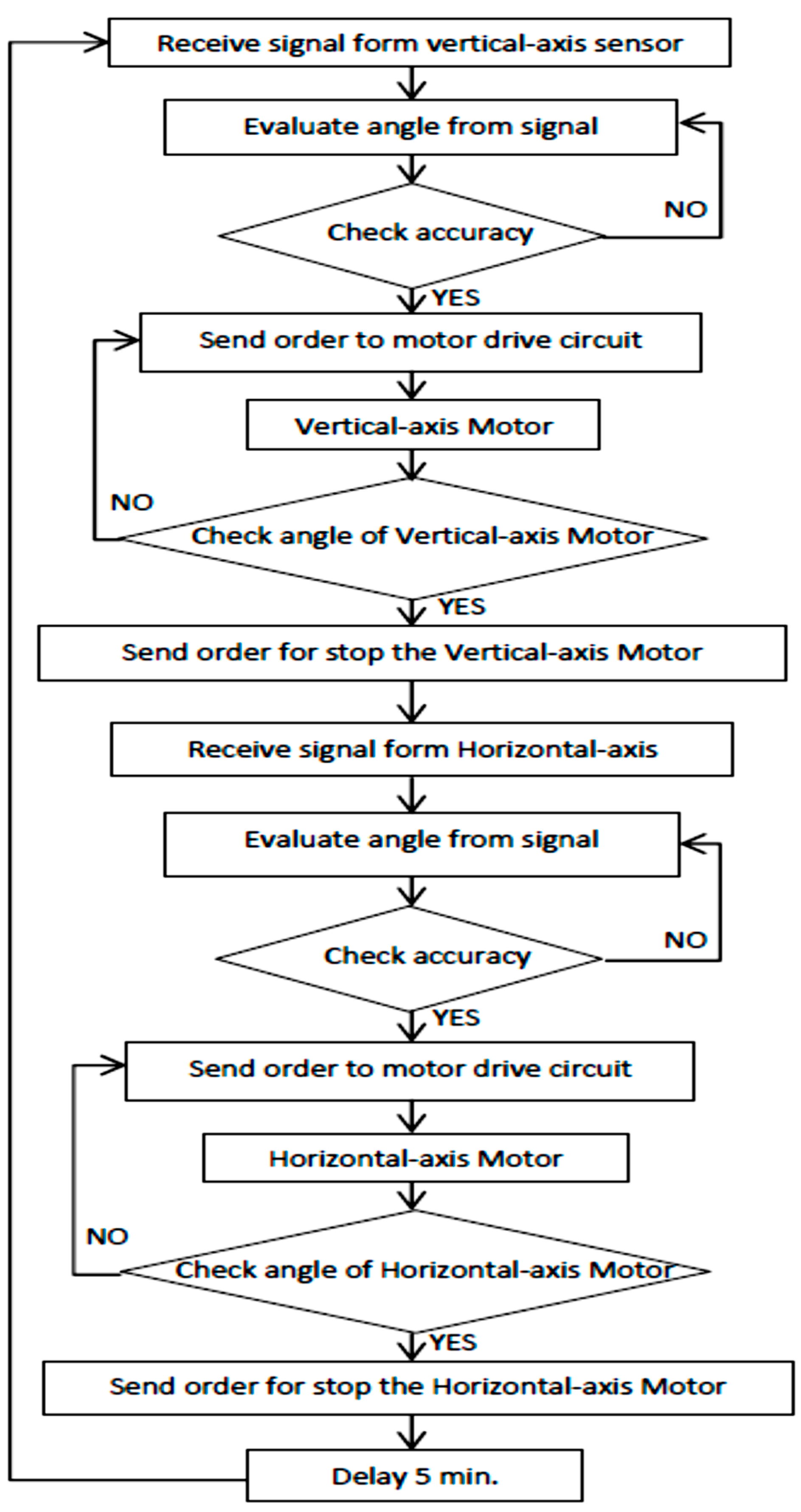
The control system for both stepping motors to drive the solar panel was designed using an Arduino microcontroller (ET-EASY MEGA 1280). The key component is the vertical and horizontal light receiver circuit, which uses an LDR device for receiving light to control the motion of the motor, processed by a microcontroller [24,25]. The design details of the light-receiving circuit are as follows:
  • The vertical light-receiving circuit causes the solar panels to move. The LDR is installed on all four sides of the light-receiving-circuit box in positions V1, V2, V3, and V4. When the LDR is exposed to sunlight, its resistance is lower, as shown in Figure 5.
Figure 5. Operation of the LDR in relation to the microcontroller for vertical movement.
Energies 16 05869 g005
Figure 5 shows the operation of the LDR in relation to the microcontroller for vertical movement. The five angle positions (0, 45, 90, 135, and 180 degrees) are controlled by tracking. When only the V1 of the LDR is detected, the angle is between 67.5 and 112.5 degrees in the east. The results showed that the vertical axis was in position at 0 degrees. Subsequently, when the Sun is at an angle between 112.5 degrees and 157.5 degrees, the V1 and V2 of LDR are detected, and signals are sent to the microcontroller causing the vertical axis to rotate to the southeast at 45 degrees. Next, the vertical axis rotates to 90 degrees only when V2 is detected and rotates to 157.5 degrees and 202.5 degrees following the operation displayed in the table in Figure 5. The vertical axis moves to a 180-degree position when exposure is at an angle between 247.5 and 292.5 degrees. However, when only V4 is detected, the vertical axis does not move, which may be due to an error in light detection. When setting up the vertical light detection unit, the V4 sensor must align with the north.
b.
The horizontal light-receiving circuit is used for the horizontal movement of the solar panel. The design shows the LDR installed in all four positions (H1, H2, H3, and H4) on top of the light-receiving circuit box. Between H1, H2, H3, and H4, there is a shading shield in the middle, separating the LDR into two sets, although all LDR light detection operates independently. Figure 6 shows the operation of the microcontroller when the LDR sends the signal for the horizontal movement of five positions (30, 60, 90, 120, and 150 degrees). At sunrise, the H1 and H2 of the LDR can detect the angle between 0 and 45 degrees horizontally with the Earth and send the signal to the microcontroller to adjust the horizontal axis to 30 degrees. When the Sun rises at an angle horizontal to the Earth between 45 and 75 degrees, H1, H2, and H4 can be detected, sending the signal to the microcontroller to adjust the horizontal axis to 45 degrees. The solar panel is perpendicular to the Earth when all horizontal LDRs (H1, H2, H3, and H4) are detected. Likewise, 120 and 150 degrees of the horizontal axis show LDR detection from the operation table presented in Figure 6. However, when all horizontal LDRs (H1, H2, H3, and H4) cannot detect sunlight, the horizontal axis does not move [25].
Figure 7 shows the circuit diagram of the five-position angles in the axis solar panel tracking system, divided into two parts: the sensor mounted on the box and the microcontroller-based control unit. The sensor box has an LDR as a light receiver, and ar1 to ar8 wires connect to the microcontroller. Figure 7a shows the light-receiving-circuit diagram of the five-position angles in the axis solar panel tracking system, in which LDR1–LDR4 represent the vertical light-receiving circuit, and LDR5–LDR8—the horizontal light-receiving circuit. The 5-V power supply for the light-receiving circuit is obtained from the microcontroller board. The resistance generated is different when the LDR is exposed to light compared to when it is not. Therefore, the adjustable resistor R1-8 is in series to the LDR in order to adjust the resistance to make it the same for easy control and processing [4]. Figure 7b shows the microcontroller circuit diagram and connecting pin for driving the stepping motor when the light-receiving circuit (ar1–ar8) is connected to the analog input of the microcontroller at pins AIN1 to AIN8, respectively [18]. The IC-STK673 uses a driver stepping motor on the vertical axis and horizontal axis, as indicated by the flowchart in Figure 8.
Figure 8 shows the working procedure of the microcontroller. Initially, when a signal is sent from the LDR to the vertical sensor, the microcontroller then estimates the angle to be used for moving the motor by checking the angle of the current. If the checked LDR signal is confirmed to be the original signal, the system will not send a signal to the drive motor. However, if it detects a new signal, the microcontroller system sends a signal to allow the stepping motor to drive the vertical-axis solar panel when the movement of the vertical-axis solar panel is 45 degrees in each cycle. The vertical-axis displacement conditions are shown in Figure 5. The microcontroller system then monitors the signal from the horizontal LDR sensor, and signal detection and control of the horizontal system are like those of the vertical system, while the moving angles between the horizontal system and the vertical system is different. The horizontal system moves 30 degrees in each cycle, as shown in Figure 6. There is a five-minute delay in the system at the start of a new round of signal detection and control.
Electrical generation was compared between the fixed solar panel system, one-axis solar panel tracking system, and two-axis solar panel tracking system, with the three methods installed in the same area. For experimental purposes, the fixed solar panel system was set at a 15-degree angle to the south. The one-axis solar panel tracking system only controlled the horizontal movement, and the solar cell panel was fixed to the south at all times. The two-axis solar panel tracking system was set up to the south in the beginning, and in sunlight conditions, the system automatically adjusted the direction of the solar panel as programmed. All four solar panels, size 12 V, 10 W, were divided into two sets connected in series. Two sets from the series were connected in parallel in order to drive a 100 W load. The 100 W load was used to test both solar panel systems by recording electrical data (voltage current and power) every 15 min from 6:00 a.m. to 6:00 p.m. via a Zupcon data logger model R3000 [23]. Data on all three systems were recorded for one year at the same time. However, Thailand experiences three distinct seasons: summer, rainy, and winter, with each season lasting approximately four months. Notably, the rainy season in Thailand occurs from July to September, spanning a period of three months [26]. Conversely, the summer season, characterized by higher solar radiation, extends from February to May.

4. Results and Discussion

The data from all three systems, collected simultaneously over the course of one year, are in Figure 9. The three systems under study included the fixed-axis solar panel system, one-axis solar tracking system, and two-axis solar tracking system, with the corresponding data being voltage, current, and power. The x-axis of the graph represents the time at which the electrical data was recorded by the data logger, spanning from 6:00 a.m. to 6:00 p.m. The data displayed for each month represents the average values of voltage, current, and power recorded.
Upon analyzing the voltage graph, it is evident that the fixed-axis system exhibited significantly lower voltage levels compared to those of the sun-tracking systems. The voltage range of the fixed-axis system during the period of 9:00 a.m. to 3:00 p.m. was approximately 15–21 V, while the solar tracking system showed a higher voltage range of approximately 16–22 V during the same period. Notably, during the timeframe of 7:00 a.m. to 9:00 a.m., the voltage of the fixed-axis system was notably lower than that of the solar tracking system. Furthermore, it is worth mentioning that both the one-axis and two-axis solar tracking systems demonstrated consistent high stability between 9:00 a.m. and 4:00 p.m.. However, after 4:00 p.m. until 6:00 p.m., the voltage levels of all three systems experienced a sharp decline. This decrease could be attributed to the combination of low irradiance and high ambient temperatures during that period.
The fixed-axis system generated a current ranging from 0.7 A to 1.1 A, whereas the tracking systems exhibited higher current values. Specifically, the one-axis solar tracking system recorded current levels of approximately 0.7 A to 1.3 A, while the two-axis solar tracking system showcased a current ranging from 0.8 A to 1.4 A. It is evident that the current of the fixed-axis solar panel system was significantly lower than that of both the one-axis and two-axis solar tracking systems [27]. However, further clarification is required to determine whether the current of the one-axis or two-axis solar panel tracking system was higher, given their similarities in performance.
Upon analyzing the power graph, it becomes evident that the graph’s characteristics in the three power conditions, fixed-axis solar panel, one-axis solar tracking, and two-axis solar tracking, exhibited behavior similar to that observed in the voltage data. Especially after 4:00 p.m., the power output of all three systems experienced a sharp decline. Furthermore, it was clear that the power generated by the fixed-axis condition was significantly lower than that of both the one-axis and two-axis solar panel tracking systems, which could be attributed to the lower voltage and current values in the fixed-axis system. However, when examining the data for both the one-axis and two-axis tracking systems, it was challenging to determine which system produced the highest power output. Therefore, the utilization of mathematical methods becomes necessary to accurately assess the voltage, current, and power of the fixed-axis, one-axis solar panel tracking, and two-axis solar panel tracking systems [28]. Additionally, it is worth noting that the graph reflects higher voltage, current, and power values during the period from March to May, primarily due to the summer season and the subsequent increase in irradiance.
However, in order to ensure effective analysis of the data, it is crucial that it is presented in a comprehensible manner. Therefore, numerical integration methods were used for analysis. These methods are preferred due to their superior suitability for weather conditions characterized by frequent partial cloud cover. Figure 10 shows the voltage, current, and power characteristics of the fixed-axis system, one-axis tracking system, and two-axis tracking system, based on yearly averages. The time scale on the x-axis ranges from 6:00 a.m. to 6:00 p.m. in all graphs. Nevertheless, a detailed comparison of the voltage, current, and power among the three systems can be observed in Figure 11, Figure 12 and Figure 13.

4.1. Part A. Analysis of the Energy in Each System

The voltage data in one year in the three systems could be compared in Figure 11. Figure 11 shows a voltage comparison between the fixed-axis, one-axis tracking, and two-axis tracking. The voltage of the fixed-axis system (black bar) was found to be lower than that of the one-axis and two-axis tracking systems, with the peak voltage being about 18.5 V at 2:15 p.m.; after that, the voltage decreased rapidly from 2:15 p.m. until 6:00 p.m. However, when considering the one-axis (blue line) and two-axis tracking (red line) systems, the voltage level was found to be relatively stable from 10:00 a.m. to 4:00 p.m. After 4:00 p.m., the voltage level was lower, and at the end time of 6:00 p.m., it fell to 9.0 V in both one-axis and two-axis tracking systems. In the fixed-axis system, the voltage dropped significantly after 3:00 p.m. since the solar panel was not perpendicular to the sunlight. This was different from a system in which the solar panels were controlled to remain perpendicular to the sunlight. In particular, scenarios with two-axis control had higher voltage levels than one-axis systems did [29]. However, in the two-axis tracking system, more angle control was required than in the one-axis tracking system.
The current comparison between the fixed-axis system (black bar), one-axis tracking system (blue bar), and two-axis tracking system (red bar) is in Figure 12. The current from the 100 W resistive load of the fixed-axis system was obviously lower than that of the one-axis and two-axis tracking systems, [30,31]. Of particular interest was the remarkable rise in current observed in both the one-axis and two-axis tracking systems compared to that of the fixed-axis system between 6:00 a.m. and about 9:00 a.m.. This difference was also evident in the voltage graph, as depicted in Figure 11. The noticeable difference stems from the superior ability of the sun-tracking system to effectively control the orientation of the solar panels compared to that of the fixed-panel system. Additionally, it was observed that the current of the one-axis was lower than that of the two-axis tracking system. Moreover, the graph characteristics observed after 3:00 p.m. were similar to those displayed in Figure 13 when the current in one-axis and two-axis tracking systems decreased. In comparison, the current of the fixed-core system current began to decline around 3:00 p.m., which was at a faster rate than that of the solar-tracking system due to the fixed-axis system being unable to adjust the angle of the solar panels to achieve its full potential irradiance.
The power comparison between the fixed-axis system (black bar), one-axis tracking system (blue bar), and two-axis tracking system (red bar) is shown in Figure 13. The graph is similar to those displayed in Figure 11 and Figure 12 due to power resulting from voltage and current. This confirmed that the fixed-axis system generated less power and could therefore not adjust the direction of the solar panel according to the movement of sunlight in the perpendicular direction. In a fixed-axis system, maximum power reached approximately 18 W at around 2:15 p.m.. However, power output exhibited unstable characteristics, unable to maintain a consistent level. On the other hand, the solar tracking system achieved a maximum power output of around 20–21 W, which was similar for both the one-axis and two-axis tracking systems. In addition, when comparing tracking systems, the one-axis system was found to be less effective than the two-axis system since with only one axis of rotation, it was unable to make the solar panel angle sufficiently perpendicular to the sunlight. Thus, the results confirmed that the two-axis tracking system provided more power than the other two mentioned systems did since it could adjust the angle of the solar panel in both vertical and horizontal directions, providing better orientation for the solar panel, thus enabling it to be perpendicular to the sunlight [19,32,33,34].
The area under a power curve generates energy in watt-hour (Wh) units. It was confirmed that the areas under a power angle for the fixed-axis system, one-axis tracking system, and 2twoaxis tracking system were about 153.47 Wh, 183.12 Wh, and 199.79 Wh, respectively. Thus, it can be confirmed that the two-axis tracking system generated the most electrical power. Nevertheless, it was necessary to consider the energy used in driving the motor. In the one-axis tracking system, the motor and controller operated eight times per day, while the two-axis tracking system was in operation 16 times per day. Hence, it was observed that the energy required for driving the motor and controller of the two-axis tracking system must have been double that of the one-axis tracking system. In order to obtain the total energy required, the energy obtained must be subtracted from that used for driving and control.

4.2. Part B. Analysis of the Relationship between Irradiation and Tracking Angles

Thailand is located near the equator. According to information from the Ministry of Energy of Thailand, each year, the country receives the potentially highest irradiation between April and May, with values ranging from 5.56 to 6.67 kWh/m2 per day. The average irradiation across Thailand from all areas equates to 5.05 kWh/m2 per day. Figure 14 shows the country’s altitude and azimuth angles in one year. The azimuth in the north is set at 0 degrees, resulting in the east, south, and west angles being 90, 180, and 270 degrees, respectively [35]. Additionally, the altitude angle can be represented within a circle diagram with each circle increasing by 10 degrees. The lines in the figure represent the Sun’s movement at different times over a 12-month period. Other time markers are shown within the lines, and depicted in green, yellow, pink, red, and black, representing 6:00, 9:00, 12:00, 15:00, and 18:00, respectively. It can be observed that the azimuth and altitude angles differ according to the month and time. The line characteristic for December is confirmed as the straightest, while June is curved.
The relationship between time and degrees using a microcontroller within a 12-month period in Thailand is presented in Table 2. This data, obtained from the two-axis solar tracking system, refers to the time interval from 6:00 a.m. to 7:00 p.m. within a 12-month period. When the LDR sensor received the signal according to the control system in Figure 8, the system controlled the vertical and horizontal axis within five steps. The five steps of angles for both the vertical and horizontal axis are related to the azimuth and altitude angles shown in Figure 5 and Figure 6, respectively. Table 2a shows the angle of the vertical axis in the sun-tracking system for every month of the year. At 6:00 a.m., the vertical axis rotated at an angle of 0 degrees (east), while at 7:00 p.m., it rotated at an angle of 180 degrees (south). The vertical axis of the solar-tracking system was rotated from 0 degrees to 180 degrees every day and reversed from 180 degrees to 0 degrees the next day. Thus, each day, the system was driven a total of eight times (four times from 0 degrees to 180 degrees, and four times from 180 degrees to 0 degrees). In addition, within a 12-month period, the rotation direction of 0 and 180 degrees was observed to occur more frequently than in any other direction [11,36,37,38].
Furthermore, Table 2b shows the solar tracking angles on the horizontal axis for each month of the year. The horizontal axis was 30 degrees at 6:00 a.m. and 150 degrees at 5:00 p.m. In the morning of the next day, the horizontal axis returned to its original position; at an angle of 30 degrees. In every month of the year, the horizontal axis rotated four times from morning to evening from 30–60, 60–90, 90–120, and 120–150 degrees at different times each month. However, in the morning, when sunlight was detected by the sensor, it caused the horizontal axis to rotate back from 150 degrees to 30 degrees (four times). The energy for the horizontal allowed the axis to be driven eight times per day. The comparison of energy production by different PV systems ( P V ) is shown in Equation (4), where ET is the energy generated by solar tracking, EPV is the energy of a fixed system without solar tracking, and EC is the energy consumption of the tracking mechanism [39].
P V = ( E T ( E P V + E C ) ) E P V × 100
The relationship between irradiance and energy driving the one-axis and two-axis systems, for just one day in December 2021 and June 2022, respectively, is shown in Figure 15a,b. Nevertheless, in Figure 14, the azimuth and altitude angles in December and June are represented by the lines in the lower and upper margins, respectively. The drive unit consists of a microcontroller and a stepping motor. As can be observed from Figure 14, the intersection of the altitude and azimuth angles form lines in December and June, appearing as the lower and upper edges, respectively. The solar irradiance measurement was conducted using a pyranometer model PMA2144 Class II, with data recorded at intervals of 20 min using a Wisco model DL2200 data logger. Irradiance started at about 6:00 a.m. and ended at about 6:00 p.m., as indicated in Figure 14.
In addition, Figure 15a shows the data for December; the total energy consumed in driving the vertical axis eight times from the azimuth angle was 4.0 Wh per day and 1.0 Wh per day from the horizontal axis. In addition, Figure 15b shows the data for June, when the total energy consumed when driving the vertical axis and horizontal axis for eight times was also 4.0 Wh per day, the same as in December. Thus, it can be confirmed that the energy required for driving the vertical axis and horizontal axis remained the same throughout the year since each day, the azimuth and altitude angles moved from 0–180 and 30–150 degrees, respectively.
Furthermore, irradiance was found to peak at about noon, producing approximately 800 W/m2, with most of the irradiance intensity occurring between 10:00 a.m. and 2:00 p.m. It can be observed that within a year, the rotation between 0 and 180 degrees occurred more frequently than in any other direction. However, during the hours from 6:00 a.m. to 10:00 a.m. and from 2:00 p.m. to 6:00 p.m., irradiance was less intense, representing one quarter of the total period using integrals. According to Table 2a, between 10:00 a.m. and 2:00 p.m. in April to August, a slight change occurs in the azimuth angle. It can be observed that during these times and months, there are very few times when the Sun passes through azimuth angles of 90 and 135 degrees. On the other hand, when considering Table 2b, during these times and months, the altitude angle changes markedly. Therefore, it may not be necessary to rotate the vertical axis because the azimuth angle changes slightly from the altitude angle. However, the energy required to drive the systems of the vertical axis and horizontal axis cannot be reduced since they need to move eight times a day in every month of the year. Therefore, it was interesting to analyze the efficiency of the system according to Equation (4) when the energy consumption data for driving the vertical and horizontal axis has been examined [40].

4.3. Part C. Analysis of the Sun-Tracking System

A comparison between the energy generated and consumed in driving the three systems of the one year could be present as show Figure 16. The green bar represents the energy generated from the fixed-axis system, one-axis tracking system, and two-axis tracking systems, namely 153.47 Wh, 183.12 Wh, and 199.79 Wh, respectively, as presented in Figure 13. Additionally, the orange bar refers to the power used to drive the movement of the solar panel, as indicated in Figure 15. However, the solar panels were required to move eight times and 16 times per day in the one-axis and the two-axis tracking systems, respectively. Therefore, the energy for driving the one-axis and two-axis tracking systems was 4 Wh and 8 Wh per day, respectively. Since the fixed system could not move the solar panel, no energy was required; thus, the drive consumed zero power. On the other hand, the one-axis and two-axis tracking systems required energy to move the solar panels using the drive unit. Accordingly, the total power of the fixed-axis system, one-axis tracking system, and two-axis tracking system was about 153.47 Wh, 179.12 Wh, and 191.79 Wh, respectively. Consequently, the energy production of the one-axis tracking system and the two-axis tracking system, when compared to that of the fixed-axis system, exhibited an increase of 16.71% and 24.97% respectively. Furthermore, the energy production of the two-axis system was 8.13% higher than that of the one-axis tracking system [41].

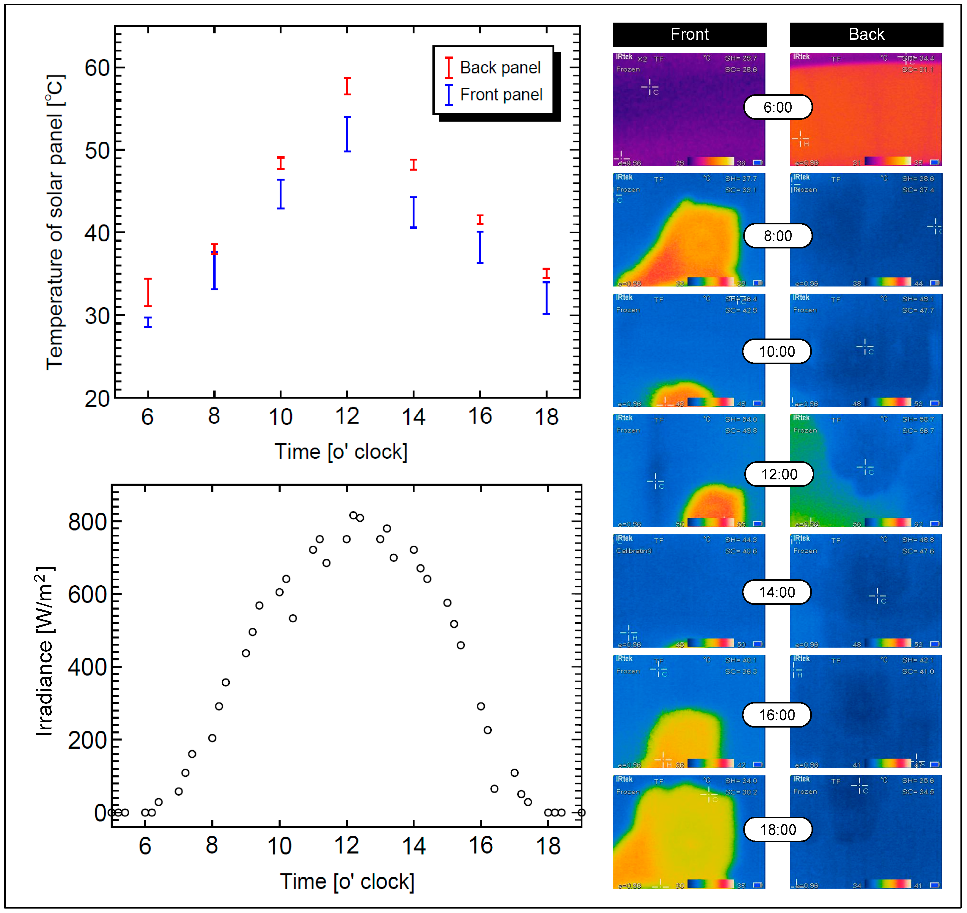
4.4. Part D. Analysis of the Solar Panel Temperature

A comparison between the temperature of the solar panel and irradiance is shown Figure 17. The figure displays three components: a photograph illustrating the temperature of the solar panel, a thermal graph depicting the temperature variations of the solar panels, and a depiction of irradiance. Temperature photographs of the solar panels were captured at 2 h intervals from 6:00 a.m. to 6:00 p.m., encompassing images taken from both the front and back sides of the solar panels. Based on the photographic data, when plotting the relationship between solar panel temperature and time, it was observed that the temperature on the back side of the solar panel exceeded that of the front side panel. The highest temperatures were recorded at noon, with readings of approximately 56–58 degrees Celsius on the back side of the solar panels and 49–54 degrees Celsius on the front side. At 6:00 a.m. and 6:00 p.m., the temperatures were similarly low, measuring around 28–34 degrees Celsius at the back side of the solar panel and 31–35 degrees Celsius at the front side. It was confirmed that there existed a temperature difference of approximately 40 degrees Celsius between the lowest and highest recorded temperatures. It was observed that the generated heat corresponded consistently to the irradiance during each period, as recorded by the pyranometer. The maximum irradiance measured was 800 W/sq.m. at noon. It has been recorded that each 1 °C increase in temperature from 25 °C resulted in a decrease in solar cell efficiency ranging from 0.3% to 0.5% [42]. Therefore, at noon, the time when the temperature was at its highest, the solar cell efficiency experienced a decrease of approximately 12%. However, the average temperature of approximately 40 degrees Celsius resulted in a solar cell efficiency decrease of around 6%. Hence, the energy production of the one-axis tracking system should increase from 16.71% to about 22.71%, and that of the two-axis tracking system should increase from 24.97% to 30.97% when operating at a temperature of 25 degrees Celsius. However, considering the actual usage in the tropical climate of Thailand, it is unlikely that the temperature will fall to 25 degrees Celsius. Therefore, the energy production of the one-axis tracking system was 16.71%, while that of the two-axis tracking system achieved a practical efficiency of 24.97%.

5. Conclusions

One-axis and two-axis solar panel tracking systems, operating on the principle of simultaneously adjusting four panels, had the capacity to generate higher voltage, current, and power compared to those of a fixed solar panel system under identical conditions. The drive unit was controlled by a microcontroller to move the solar panels using a stepping motor 16 times/day and eight times/day in the two-axis and one-axis tracking systems, respectively. The driving energy of the one-axis tracking system was half that of the two-axis tracking system. Consequently, the power used in driving the one-axis and two-axis tracking systems was 4 Wh/day and 8 Wh/day, respectively. Very little energy was consumed in moving the solar panels because the vertical or horizontal axis drive used energy only eight times per day, unlike in an all-time solar tracking system. In addition, when electrical energy from the five-position angles in a Sun-tracking system using one axis or two axes was subtracted from the electrical power of the drive system, it still generated more energy than that lost in the drive unit due to the control technique used in the five-position angles of the Sun-tracking system. Therefore, the energy production of the one-axis and two-axis systems was 16.71% and 24.97%, respectively. The difference in energy production between the one-axis and two-axis systems was 8.26%, which could be considered significant. Energy production depends on geographical location and the energy consumed by the drive system. Since Thailand is located near the equator, very small shifts occur in the azimuth and altitude angles. A small change in both angles results in less energy being required to drive the vertical and horizontal axes. Furthermore, the five-position angle Sun-tracking technique requires less energy for the tracking mechanism than is the case of an all-time solar tracking system.

Author Contributions

Conceptualization, N.T. and T.Y.; Methodology, N.T. and H.K.; Validation, N.T., W.P. and S.A.; Formal analysis, N.T., T.S. and N.K.; Investigation, N.T., A.C., T.T., N.M. and S.A.; Resources, A.S.; Funding acquisition, N.M., N.K. and S.A.; Writing—original draft, N.T. and N.M.; Writing—review & editing, N.T., N.K. and S.A.; Visualization, N.T., T.M. and S.N.; Supervision, N.M. All authors have read and agreed to the published version of the manuscript.

Funding

This work was supported by King Mongkut’s University of Technology Thonburi (KMUTT), Thailand, and under the project of the Research, Innovation, and Partnerships Office (RIPO) with the Faculty of Industrial Education and Technology Research Funding.

Data Availability Statement

The data presented in this study are available on request from the corresponding authors.

Conflicts of Interest

The authors declare no conflict of interest.

References

  1. Al-Amin, M.; Chowdhury, N.B.; Rabby, F.; Banik, S.C.; Islam, Z. Study of Construction and Analysis of a vehicle using Solar energy with Solar Tracking System. Int. J. Nov. Res. Electr. Mech. Eng. 2014, 1, 44–50. [Google Scholar]
  2. Sharma, C.; Sharma, A.K.; Mullick, S.C.; Kandpal, T.C. Assessment of solar thermal power generation potential in India. Renew. Sustain. Energy Rev. 2015, 42, 902–912. [Google Scholar] [CrossRef]
  3. Charafeddine, K.; Tsyruk, S. Automatic Sun-Tracking System. In Proceedings of the 2020 International Russian Automation Conference (RusAutoCon), Sochi, Russia, 29 September 2020. [Google Scholar]
  4. Kumar, V.S.S.; Suryanarayana, S. Automatic Dual Axis Sun Tracking System using LDR Sensor. Int. J. Curr. Eng. Technol. 2014, 4, 3214–3217. [Google Scholar] [CrossRef] [Green Version]
  5. Thungsuk, N.; Mungkung, N.; Tanaram, T.; Chaithanakulwat, A.; Arunrungsusmi, S.; Poonthong, W.; Songruk, A.; Tunlasakun, K.; Chunkul, C.; Tanitteerapan, T.; et al. The Characterization Analysis of the Oil-Immersed Transformers Obtained by Area Elimination Method Design. Appl. Sci. 2022, 12, 3970. [Google Scholar] [CrossRef]
  6. Theraja, B.L.; Theraja, A.K. A Text Book of Electrical Technology; AC & DC Machines in S.I: New Delhi, India; Volume 2.
  7. Wang, Q.; Zhang, J.; Hu, R.; Shao, Y. Automatic Two Axes Sun-Tracking System Applied to Photovoltaic System for LED Street Light. Appl. Mech. Mater. 2010, 43, 17–20. [Google Scholar] [CrossRef]
  8. Ponciano, V.D.F.G.; Ponciano, I.D.M.; Alves, D.G.; Saretta, E.; Coelho, R.D. Conversion of solar photovoltaic energy into hydraulic energy applied to irrigation systems using a manual sun tracking. Irrig. Drain. 2020, 25, 508–520. [Google Scholar] [CrossRef]
  9. Rizi, A.P.; Ashrafzadeh, A.; Ramezani, A. A financial comparative study of solar and regular irrigation pumps: Case studies in eastern and southern Iran. Renew. Energy 2019, 138, 1096–1103. [Google Scholar] [CrossRef]
  10. Nadia, A.R.; Isa NA, M.; Desa MK, M. Efficient single and dual axis solar tracking system controllers based on adaptive neural fuzzy inference system. J. King Saud Univ. -Eng. Sci. 2020, 32, 459–469. [Google Scholar]
  11. Al-Rousan, N.; Isa, N.A.M.; Desa, M.K.M. Advances in solar photovoltaic tracking systems: A review. Renew. Sustain. Energy Rev. 2018, 82, 2548–2569. [Google Scholar] [CrossRef]
  12. Akbar, H.S.; Siddiq, A.I.; Aziz, M.W. Microcontroller based dual axis sun tracking system for maximum solar energy generation. Am. J. Energy Res. 2017, 5, 23–27. [Google Scholar]
  13. Maharaja, K.; Xavier, R.J.; Amla, L.J.; Balaji, P.P. Intensity based dual axis solar tracking system. Int. J. Appl. Eng. Res. 2015, 10, 19457–19465. [Google Scholar]
  14. Huang, C.-H.; Pan, H.-Y.; Lin, K.-C. Development of Intelligent Fuzzy Controller for a Two-Axis Solar Tracking System. Appl. Sci. 2016, 6, 130. [Google Scholar] [CrossRef] [Green Version]
  15. Hijawi, H.; Arafeh, L. Design of dual axis solar tracker system based on fuzzy inference systems. Int. J. Soft Comput. Artif. Intell. Appl. 2016, 2016 5, 23–35. [Google Scholar] [CrossRef]
  16. Homadi, A.; Hall, T.; Whitman, L. Using solar energy to generate power through a solar wall. J. King Saud Univ. -Eng. Sci. 2020, 32, 470–477. [Google Scholar] [CrossRef]
  17. Kalogirou, S.A. Solar Energy Engineering Processes and Systems, 2nd ed.; Academic Press (Elsevier): Cambridge, MA, USA, 2014; ISBN 978-0-12-397270-5. [Google Scholar]
  18. Mahdavi, M.; Li, L.; Zhu, J.; Mekhilef, S. An adaptive Neruo-Fuzzy controller for maximum power point tracking of photovoltaic systems. In Proceeding of the IEEE Region 10 Conference TENCON, Macao, China, 1–4 November 2015. [Google Scholar]
  19. Hariri, N.G.; AlMutawa, M.A.; Osman, I.S.; AlMadani, I.K.; Almahdi, A.M.; Ali, S. Experimental Investigation of Azimuth- and Sensor-Based Control Strategies for a PV Solar Tracking Application. Appl. Sci. 2022, 12, 4758. [Google Scholar] [CrossRef]
  20. Angulo-Calderón, M.; Salgado-Tránsito, I.; Trejo-Zúñiga, I.; Paredes-Orta, C.; Kesthkar, S.; Díaz-Ponce, A. Development and Accuracy Assessment of a High-Precision Dual-Axis Pre-Commercial Solar Tracker for Concentrating Photovoltaic Modules. Appl. Sci. 2022, 12, 2625. [Google Scholar] [CrossRef]
  21. Ruelas, J.; Muñoz, F.; Lucero, B.; Palomares, J. PV Tracking Design Methodology Based on an Orientation Efficiency Chart. Appl. Sci. 2019, 9, 894. [Google Scholar] [CrossRef] [Green Version]
  22. Sharma, M.; Gupta, S. Adaptive neuro fuzzy inference system technique for photovoltaic array systems. Sol. Energy Mater. Sol. Cells 2015, 46, 1229–1245. [Google Scholar]
  23. Reddy, K.H.; Ramasamy, S.; Ramanathan, P. Hybrid adaptive neuro fuzzy based speed controller for brushless DC motor. Gazi Univ. J. Sci. 2017, 30, 93–110. [Google Scholar]
  24. Kiyak, E.; Gol, G. A comparion of fuzzy logic and PID controller for a single-axis solar tracking system. Renew Wind. Water Sol. 2016, 3, 7. [Google Scholar] [CrossRef] [Green Version]
  25. Aleem, A.; El-Sharief, M.A.; Hassan, M.A.; El-Sebaie, M.G. Implementation of Fuzzy and Adaptive Neuro-Fuzzy Inference Systems in Optimization of Production Inventory Problem. Appl. Math. Inf. Sci. 2017, 11, 289–298. [Google Scholar] [CrossRef]
  26. Kuttybay, N.; Mekhilef, S.; Saymbetov, A.; Nurgaliyev, M.; Meiirkhanov, A.; Dosymbetova, G.; Kopzhan, Z. An Automated Intelligent Solar Tracking Control System with Adaptive Algorithm for Different Weather Conditions. In Proceedings of the 2019 IEEE International Conference on Automatic Control and Intelligent Systems (I2CACIS), Shah Alam, Malaysia, 29 June 2019; pp. 315–319. [Google Scholar]
  27. Sidek, M.; Azis, N.; Hasan, W.; Ab Kadir, M.; Shafie, S.; Radzi, M. Automated positioning dual-axis solar tracking system with precision elevation and azimuth angle control. Energy 2017, 124, 160–170. [Google Scholar] [CrossRef]
  28. Seme, S.; Srpčič, G.; Kavšek, D.; Božičnik, S.; Letnik, T.; Praunseis, Z.; Štumberger, B.; Hadžiselimović, M. Dual-axis photovoltaic tracking system-design and experimental investigation. Energy 2017, 139, 1267–1274. [Google Scholar] [CrossRef]
  29. Maiga, A. Theoretical Comparative Energy Efficiency Analysis of Dual Axis Solar Tracking Systems. Energy Power Eng. 2021, 13, 448–482. [Google Scholar] [CrossRef]
  30. Allw, A.S.; Shallal, I. Evaluation of Photovoltaic Solar Power of a Dual-Axis Solar Tracking System. J. Southwest Jiaotong Univ. 2020, 55. [Google Scholar] [CrossRef]
  31. Ferdaus, R.A.; Mohammed, M.A.; Rahman, S.; Salehin, S.; Mannan, M.A. Energy Efficient Hybrid Dual Axis Solar Tracking System. J. Renew. Energy 2014, 2014, 629717. [Google Scholar] [CrossRef]
  32. Awasthi, A.; Shukla, A.K.; S.R., M.M.; Dondariya, C.; Shukla, K.N.; Porwal, D.; Richhariya, G. Review on sun tracking technology in solar PV system. Energy Rep. 2020, 6, 392–405. [Google Scholar] [CrossRef]
  33. Batayneh, W.; Bataineh, A.; Soliman, I.; Hafees, S.A. Investigation of a single-axis discrete solar tracking system for reduced actuations and maximum energy collection. Autom. Constr. 2019, 98, 102–109. [Google Scholar] [CrossRef]
  34. Seme, S.; Štumberger, B.; Hadžiselimović, M.; Sredenšek, K. Solar Photovoltaic Tracking Systems for Electricity Generation: A Review. Energies 2020, 13, 4224. [Google Scholar] [CrossRef]
  35. Farrar-Foley, N.; Rongione, N.A.; Wu, H.; Lavine, A.S.; Hu, Y. Total solar spectrum energy converter with integrated pho-tovoltaics, thermos-electrics, and thermal energy storage: System modeling and design. Int. J. Energy Res. 2021, 46, 5731–5744. [Google Scholar] [CrossRef]
  36. Gbadamosi, S.L. Design and implementation of IoT-based dual-axis solar PV tracking system. Przegląd Elektrotechniczny 2021, 2021, 57. [Google Scholar] [CrossRef]
  37. Hamad, B.A.; Ibraheem, A.M.; Abdullah, A.G. Design and Practical Implementation of Dual-Axis Solar Tracking System with Smart Monitoring System. Przegląd Elektrotechniczny 2020, 96. [Google Scholar] [CrossRef]
  38. SKivrak, S.; Gunduzalp, M.; Dincer, F. Theoretical and experimental performance investigation of a two-axis solar tracker under the climatic condition of Denizil, Turkey. Przegląd Elektrotechniczny 2012, 88, 332–336. [Google Scholar]
  39. Kuttybay, N.; Saymbetov, A.; Mekhilef, S.; Nurgaliyev, M.; Tukymbekov, D.; Dosymbetova, G.; Meiirkhanov, A.; Svanbayev, Y. Optimized Single-Axis Schedule Solar Tracker in Different Weather Conditions. Energies 2020, 13, 5226. [Google Scholar] [CrossRef]
  40. Božiková, M.; Bilčík, M.; Madola, V.; Szabóová, T.; Kubík, Ľ.; Lendelová, J.; Cviklovič, V. The Effect of Azimuth and Title Anglea. Changes on the Energy Balance of Photovoltaic System Installed in the Southern Slovakia Region. Appl. Sci. 2021, 11, 8998. [Google Scholar] [CrossRef]
  41. Orłowski, P. Analysis of two-criteria optimization problem with application to automatic orders control system for inventory with long-delay supply with feedback—Feedforward controller and Smith predictor. Przegląd Elektrotechniczny 2016, 92, 218–221. [Google Scholar]
  42. Utomo, B.R.; Sulistyanto, A.; Riyadi, T.W.B.; Wijayanta, A.T. Enhanced Performance of Combined Photovoltaic–Thermoelectric Generator and Heat Sink Panels with a Dual-Axis Tracking System. Energies 2023, 16, 2658. [Google Scholar] [CrossRef]
Figure 1. The angle when the Sun moves across from sunrise to sunset.
Energies 16 05869 g001
Figure 2. Solar angle diagram.
Energies 16 05869 g002
Figure 3. The five-position angle axis controlled by the solar panel tracking system. (a) Three-dimensional program design; (b) solar panel when installed with the structure.
Energies 16 05869 g003
Figure 6. Operation of the LDR in relation to the microcontroller for horizontal movement.
Energies 16 05869 g006
Figure 7. Circuit diagram of the five-position angles axis solar panel tracking system. (a) Light-receiving circuit diagram; (b) microcontroller circuit diagram.
Energies 16 05869 g007
Figure 8. Microcontroller procedure.
Energies 16 05869 g008
Figure 9. Data in one year of voltage, current, and power in the three systems.
Energies 16 05869 g009
Figure 10. The average data in one year of voltage, current, and power in the three systems.
Energies 16 05869 g010
Figure 11. Voltage comparison between the three systems.
Energies 16 05869 g011
Figure 12. Current comparison between the three systems.
Energies 16 05869 g012
Figure 13. Power comparison between the three systems.
Energies 16 05869 g013
Figure 14. Altitude and azimuth angles over a 12-month period in Thailand.
Energies 16 05869 g014
Figure 15. Relationship between irradiance and driving energy of the solar tracking system.
Energies 16 05869 g015
Figure 16. Comparison between the energy generated and that required for driving the three systems.
Energies 16 05869 g016
Figure 17. Comparison between the temperature of the solar panel and irradiance.
Energies 16 05869 g017
Table 1. Technology used in related trackers.
Axis TrackerTracker SensorTypeControlRef.
Single-axisLDRAll time trackerPID control[19]
Dual-axismicro-electromechanical solar sensorAll time trackerArduino board in a closed-loop control[20]
Dual-axis-3-point trackerFPGA boards[21]
Table 2. Relationship between time and degree of control by the microcontroller over a 12-month period in Thailand.
Energies 16 05869 i001Energies 16 05869 i002
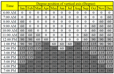
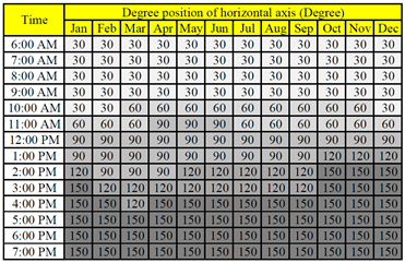
(a) Degree position of the vertical axis(b) Degree position of the horizontal axis
Disclaimer/Publisher’s Note: The statements, opinions and data contained in all publications are solely those of the individual author(s) and contributor(s) and not of MDPI and/or the editor(s). MDPI and/or the editor(s) disclaim responsibility for any injury to people or property resulting from any ideas, methods, instructions or products referred to in the content.

