Abstract
The present paper treats a black-box estimation of the three independent parameters of a reciprocal lossy two-port network whose terminals are supposed to be accessible to an impedance measurement device. The discussed estimation method is based on the availability of a number of data pairs made of external load admittances paired to equivalent external admittances affected by measurement errors. The proposed method is framed as a squared-estimation-error minimization problem that leads to a system of three nonlinear equations in the three unknown parameters. A key observation is, however, that a core subsystem of two equations may be turned exactly to a linear form and hence may be solved in closed form. The purely real-valued case is treated first since it serves to clarify the optimization problem at hand and the structure of its solution. In the purely real-valued case, a statistical analysis is carried out as well, which affords the evaluation of the effects of the measurement errors. The results of the statistical analysis afford quantifying the dependence of the estimation errors from the number of samples and from the variance of the measurement errors. Subsequently, the full complex-valued case is treated. Results of numerical simulations complement and illustrate the theoretical findings. The obtained numerical results confirm the statistical analysis and that the proposed external identification method is effective.
1. Introduction
Linear two-port and multiport networks have found widespread application in engineering and in applied sciences to model multivariable interaction phenomena. A recent reference on multiport networks and on their energy-exchange properties published on Energies is [1], while a general-purpose textbook that includes multiport elements is [2].
Multiport networks have been used in the modeling of complex mechanical systems [3], in waveguides modeling and calibration [4] as well as in antennas modeling and optimization [5], in modeling bioheat transfers in lungs (in particular during thoracic and open-heart surgery) [6], in the analysis of power delivery in electrical railways systems [7], in modeling low dropout voltage regulators [8] as well as in modeling and analyzing multiple grid-connected voltage source converter systems [9], in the modeling of electrochemical transport processes through biological membranes [10], as well as in the modeling and simulation of acoustic systems [11] even by two-port circuit models derived from the linearized Navier–Stokes equations [12]. In addition, nonlinear multiterminal electronic devices or portions of electronic circuits may be represented, in the small-signal hypothesis, as linear multiport networks.
Most black-box modeling techniques of linear interaction phenomena involve two-port circuits. However, multiport circuit models are of prime importance when a large number of variables are involved in an interaction phenomenon. As a specific application to exemplify the usefulness of multiport identification, consider the electronic chip package/connector de-embedding problem tackled in [13]. The plastic package of an electronic chip embeds a number of highly conductive wires whose function is to connect the internal electronic chip to the external pins. At very high frequencies (in the range of GHz), a number of parasitic effects show up and, in particular, the connecting wires interact to each other electromagnetically in such a way that they may no longer be regarded as simple wires. In [13], the package is modeled as a reciprocal, linear, time-invariant multiport network, which is supposed to be accessible by n internal electrical ports and n external electrical ports. The identification of the circuit model, represented through its admittance matrix, is carried out by measuring the admittance of the external ports by a vector network analyzer. Once identified, the model is used to de-embed the internal chip, namely, to decouple the signals to/from the chip’s pins which become mixed up by the connector. A further example concerns modeling microvascular networks [14], where two-port models are used to compute biohydraulic quantities related to fluid circulation in thin blood vessels. In such an application, hence, neither the modeled phenomenon nor the variables of interest are of electric type.
Two-port networks turn out to be useful tools that afford analyzing the behavior and performance of linear networks that may be accessed by two pairs of terminals. Two-port network models are electrical circuits that embody a mathematical representation of the relationship occurring between the two independent voltages and two independent currents at their terminals. There exist six common types of two-port network models, classified as impedance, admittance, hybrid, and transmission type [15,16].
One of the challenges of using two-port network models is identifying the values of their independent parameters. There exist different methods to accomplish such a task, such as short-circuit, open-circuit, and known-load tests [2]. Each method implies applying known voltages and currents to the terminals and measuring the resulting voltages and currents. The choice of one specific method depends on the feasibility and accuracy of the available measurement devices. In the present research work, we deal specifically with the problem of the external identification of the three independent parameters of a reciprocal, lossy Y-type two-port network. Lossy networks characterize, among others, transmission media that entail some form of energy dissipation, such as energy loss due to nonideal conducting walls [17,18].
A basic assumption behind the present research is that the terminals of the two-port network are accessible to an impedance-measurement analyzer. Through such device, a number of test loads may be subjected to measurement of admittance. Next, such known loads may be connected to one of the ports of the network, and the equivalent admittance at the other port may be measured. In this way, a dataset may be collected, made of external load admittance values paired to equivalent external admittance values.
The collected data pairs are supposed to be affected by measurement errors whose entity depends on the quality of the measurement device and on the competence in the investigation. Whenever the measurement errors affecting the data available to accomplish the identification task are not negligible, the classical identification methods may be severely affected in a negative way. (In dimensions higher than two, such problem is even more severe, as illustrated, for instance, in [1].) In these instances, alternative identification methods may, hence, prove viable. A summary of three methodologies to accomplish identification are summarized in Table 1.

Table 1.
Advantages and drawbacks of three categories of external identification methods.
The method utilized to estimate the values of the parameters is based on a squared-estimation-error minimization procedure. Such formulation leads to a system of three nonlinear equations in the three (independent) unknown parameters of the Y-type two-port network model. A subsystem of two equations is then isolated, and it will be shown that such a subsystem may be turned exactly (i.e., without any approximation) to linear by an appropriate ansatz and may hence be solved in closed form.
The first part of the present paper deals with the purely real-valued case that serves to clarify the problem and the found solution. The relative simplicity of the equations pertaining to the purely real case affords a statistical analysis to quantify the effects of the measurement errors on the quality of the solution, under the form of the mean values and the variances of the deviations of the estimates to the actual values, evaluated to lowest order of approximation. In the second part of the paper, the full complex-valued case is treated, although with fewer details compared to the real-valued case since the equations are similar to the ones found for the purely real case.
The present analysis is of methodological value and does not imply any in-lab experimentation. Results of numerical simulations are hence displayed and discussed to complement and illustrate the theoretical findings throughout the paper.
2. Nomenclature Summary
The present paper includes several variables and constants. Table 2 summarizes the principal symbols used in the following sections and is meant as a guide for readers throughout the extensive notation used.
Table 2.
List of the principal symbols used within this manuscript and their description.
3. Problem Formulation for the Real-Valued Case
In the present work, we shall assume that a two-port system is represented by a impedance matrix . Since the working hypotheses are that the system being modeled is lossy, reciprocal, and memoryless, we shall assume that the matrix Y is symmetric, real-valued, and positive definite, namely, that it possesses the structure and that the following constraints on the three independent parameters hold:
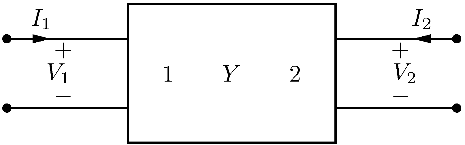
which inherently imply that as well. A diagram of a two-port is shown in Figure 1.

Figure 1.
Two-port network diagram. The symbol Y denotes the type of representation; the marks 1 and 2 denote the port number. The diagram also shows the port-1 and port-2 voltage–current pairs.
Upon loading the second port by a resistor of conductance , the equivalent conductance h at the first port reads
Notice that ; therefore, by definition of the conductance g and by virtue of the constraints (1), it holds that , namely, the whole bipole behaves as a passive resistor. Since , the above relationship may be rewritten as the following constraint on the unknown triple
Clearly one single measurement testing is not enough to determine three unknowns, nor would be three tests, because of inherent measurement errors. We shall henceforth admit a number of independent tests, which provide a set of pairs , with . Due to measurement errors, none of such pairs exactly meet the relationship (3). The discrepancy of the left-hand side to zero will be denoted as modeling error and defined as
where each and each . As a global model-to-data mismatch figure, we defined the index
Optimal estimation consists in determining the values of the two-port parameters that minimize the quadratic error J and that meet the constrains (1).
4. Closed-Form Solution to the Optimization Problem for the Real-Valued Case
The first fundamental observation is that the pairwise modeling error appears as a polynomial in the three variables x, y, and z. As a consequence, the global mismatch figure J also takes the form of a polynomial in such three variables. In fact, it takes the expression
where we introduce the following constants that depend only on the dataset :
It is interesting to underline that the constants D and E appear to be scaled versions of the sample mean value of the datasets and , respectively, and the constants C and G appear as scaled versions of the variances of the two sets, while the constant B appears as a correlation coefficient between the data sequences (up to scaling and shifting). Such observations will become useful in evaluating the positive definiteness of the Hessian matrix associated with the error function J.
It is also useful to highlight that, since any value and , any coefficient in the list (7) is also strictly positive. Such observation will turn out to be worthy in the evaluation of the shape of the feasible region.
In order to determine the critical points of the global error, it is necessary to compute the partial derivatives of the function J with respect to its three variables and to set them to zero. In order to confirm that such critical points correspond to minima of the criterion function, it will also be necessary to compute the Hessian matrix of the mismatch function J and to make sure that it is positive definite. The sought partial derivatives read
Some observations are worth highlighting. The first observation is that one trivial solution arising by setting the partial derivative to zero would be ; we shall, however, rule out such a solution that would imply the absence of interaction between the two ports, hence making the problem essentially unworthy examining. A second observation is that the variable y appears always at the power of two; such observation leads to the conclusion that, within the present framework, it is impossible to determine the right sign of the parameter y and, hence, that this method always produces two possible solutions, namely, and .
A third observation of interest is that from the equation , arising from the relation (9), we may directly express the unknown y in terms of the unknowns as
By replacing such a result back into the first equation of the system, (8), and into the third Equation (10), we may simplify the identification problem to a two-variable optimization problem. But there is more to that, since the resulting system of equations turns out to be linear and may hence be solved in closed form. In fact, the equations and lead to the linear system
where we have defined the two-variable unknown array t, the system matrix M, and the coefficients array d. Notice that the matrix M results to be symmetric.
The solution of the linear system (12) reads , where the inverse of the coefficient matrix M takes the form
with . Henceforth, the solution in closed form reads
The Hessian matrix of the global modeling error J with respect to the variables reads , hence the solution to the above linear system of equations represents a minimum of the global error only if the matrix M is positive definite. Positive definiteness of such Hessian matrix holds only if
We will verify that such constraints are, in fact, always met. The first constraint, , may be recast explicitly as . Upon defining
simple calculations show that . Analogously, upon defining
the last one being a correlation coefficient, it turns out that and that ; therefore,
Since the value of the correlation coefficient is strictly less than 1, the second constraint is unconditionally met as well.
Notice that the positive definiteness of the matrix implies the invertibility of the matrix M which, in turn, implies that linear system of Equation (12) certainly admits a solution.
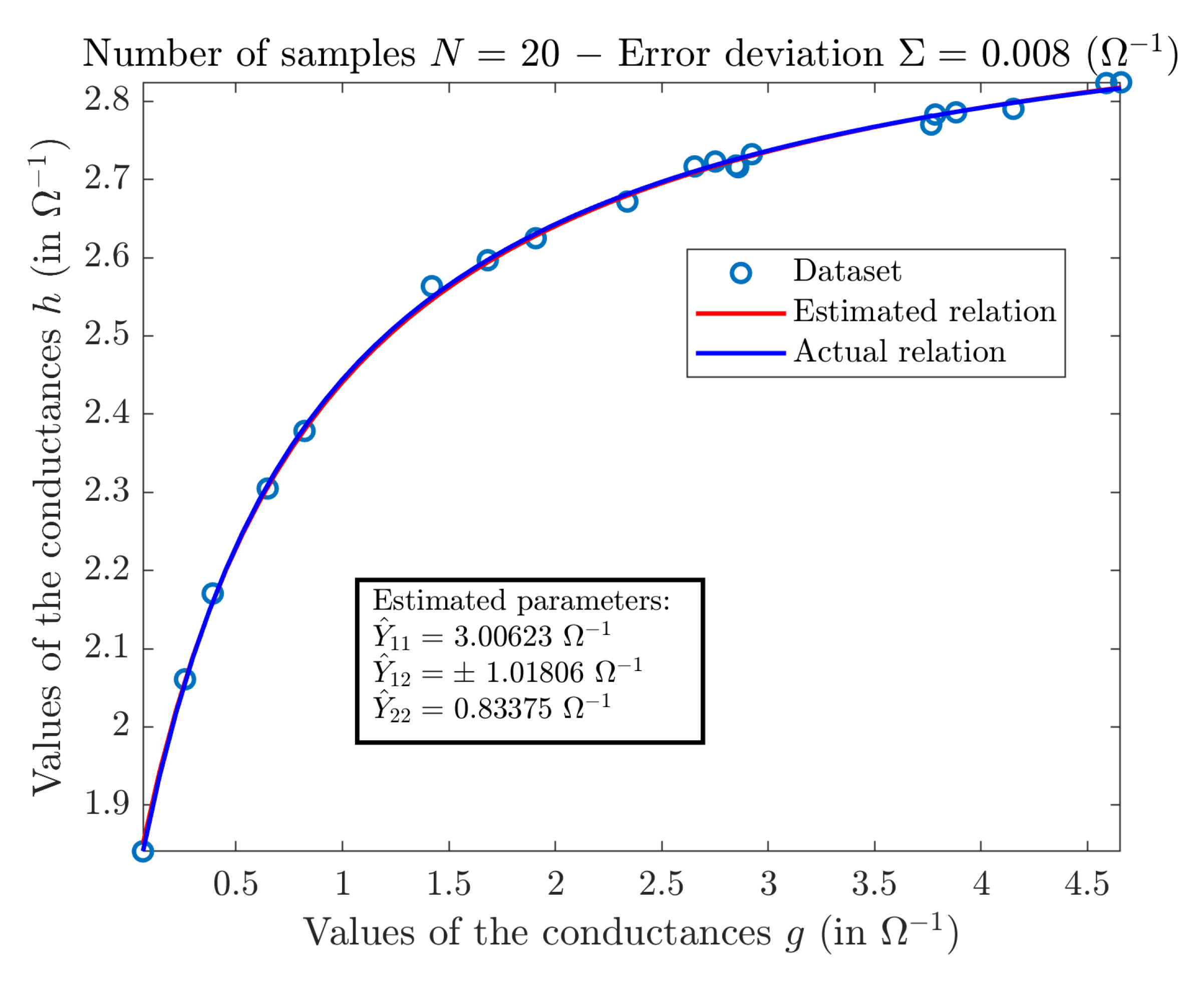
Figure 2 shows the result of a numerical test. In this test, the actual values of the parameters are , , and , and the values of g are drawn randomly from a uniform distribution in . The measurement error is herewith assumed to be a random noise with normal distribution. Namely, we shall assume that each true value is affected by an additive normal measurement error, such that the value that is effectively collected is , with and that each true value is affected by an additive normal measurement error, such that the collected value is , where . The quantity denotes the variance of the zero-mean measurement error.
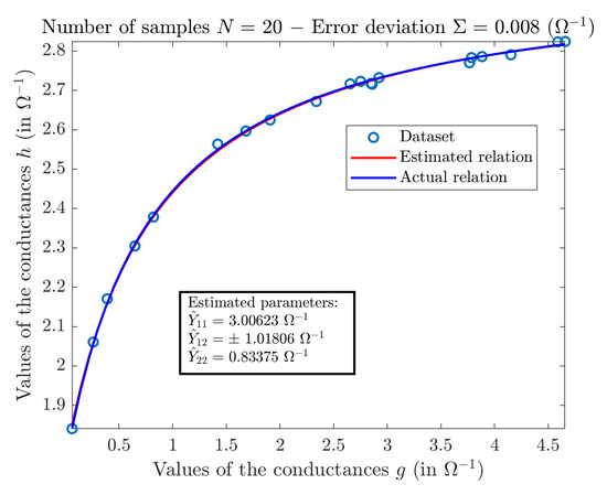
Figure 2.
Result of a numerical test in the real-valued estimation case. The estimated/actual relation refers to the function with set to the estimated values in the first case and to the actual values in the second case. Notice that the red line and the blue line are hardly distinguishable because they are almost perfectly superimposed, which testifies that the developed estimation method provides a result hardly distinguishable, in practice, from the actual values of the sought parameters.
The achieved minimal squared error is .
We further notice that the definiteness constraint may be rewritten in terms of the variables only, through the relationship (11), as
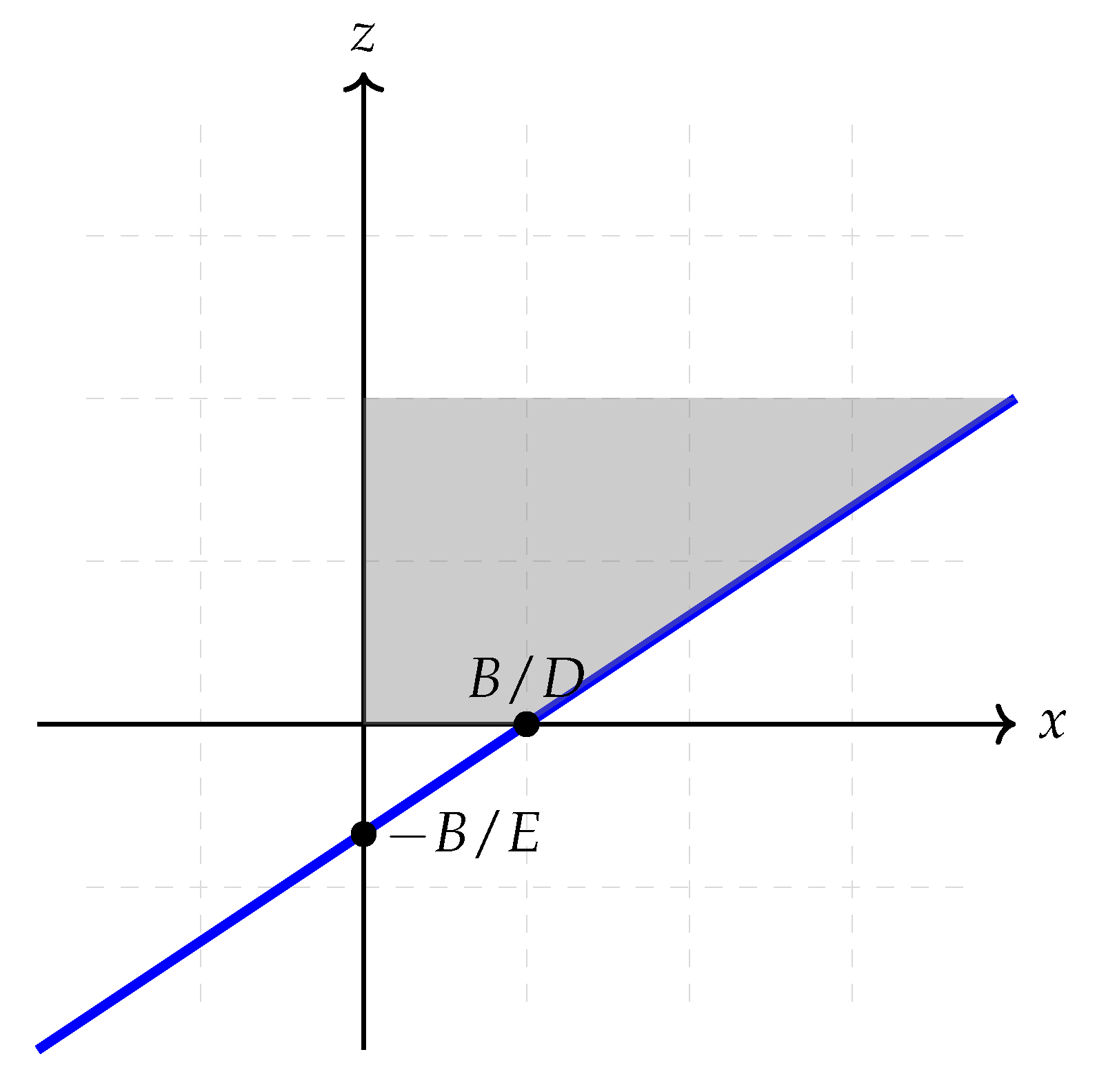
Such inequality, together with the further definiteness constraint , individuates the feasible set of acceptable solutions situated in the upper-right quadrant of the plane , as shown in Figure 3. The feasible region is characterized by the axes intercepts and (since , as recalled at the beginning of the present section). We shall remark that, in particular, whenever the actual value of z is approximately zero (yet being positive), the feasible solution for x is approximately .
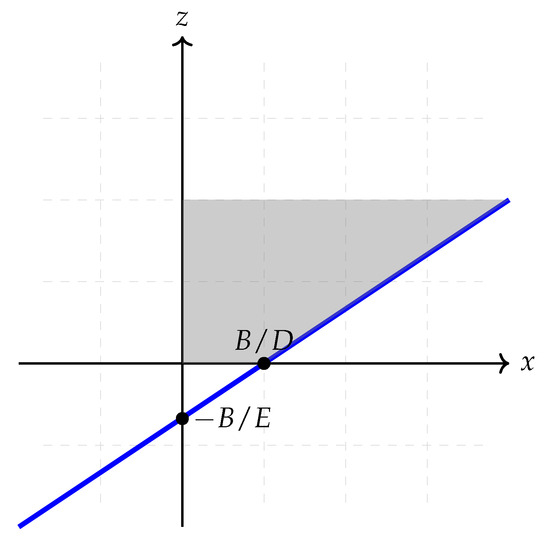
Figure 3.
Shape of the feasible region in the x–z plane in gray color.
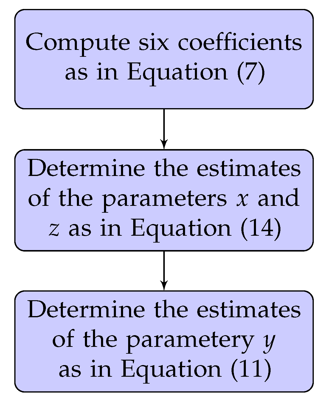
The proposed external identification approach, resulting from the above mathematical developments, is summarized by the flowchart displayed in Figure 4.
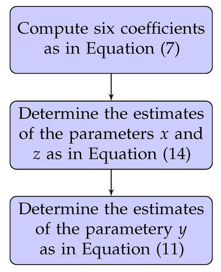
Figure 4.
Flowchart summary of the proposed external identification approach.
5. Special Case of the Parameter Known in the Real-Valued Case
A special measurement setting may be exploited to obtain an approximation of the parameter of the two-port. In the following, we make a number of assumptions to formalize such a special case:
- The second port of the two-port network may be closed by a short-circuit, which corresponds to assuming ; notice that this is an assumption that does not necessarily correspond to a real-world case since, at high frequency, a short-circuit is not necessarily so.
- The equivalent conductance h, in this particular measurement setting, may be measured with negligible measurement error; even this assumption will, most likely, appear just as a case study.
Under the above assumptions, the fundamental relationship (2) returns , namely, the value of the variable x may be measured directly and hence is to be considered, in principle, as known.
Now, before presenting the resulting closed-form expression of the variable z, it pays to define a reduced error function that is obtained by plugging the relation (11) into the error function (6) to obtain
If the value of the parameter x is known, the reduced error function is a function of the variable z only, whose optimal value is obtained by setting , which gives
Aside, we deem it quite interesting the observation that the sharpness of the paraboloid described by the function along both axes is determined by the two coefficients and that are proportional to the sample variance of the data subsets and .
Moreover, we notice that if the physical system that is being modeled by a two-port network allows swapping of the first port with the second port, namely, the first port may be loaded on a known load and the second port is accessible for conductance measurement, then the above considerations may be repeated with the assumption that the parameter be known. In this way, both parameters and may be measured directly and the remaining parameter , the transfer admittance, may be estimated through a series of further measurements.
6. Statistical Analysis for the Real-Valued Case
The present analysis is based on the assumption that the measurements are the realizations of a random variable g and that the measurements are the realizations of a random variable h. We may then define a new error-type random variable
On the basis of such assumption, we shall be able to estimate a number of statistical characteristics of the modeling error and of the deviations of the parameters estimations to their actual values.
6.1. Statistical Analysis of the Modeling Error
It is instrumental to estimate the average value and the variance of the error variable .
With regard to the average value, it holds that
where we make use of the statistical expectation operator .
The actual average values may be estimated through the relevant coefficients (7) normalized by the integer N, namely, to first order
We already showed in Section 4 that the quantity equals when the triple is the one estimated by the devised optimization algorithm; therefore, it holds that .
Likewise, the variance of the error-type random variable may be approximated, to first order, as
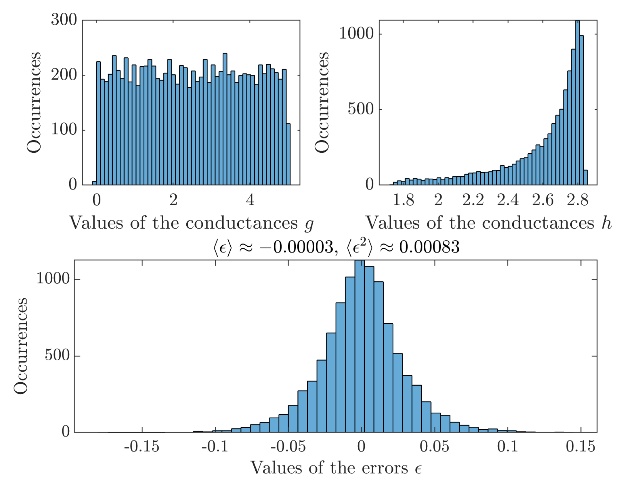
Figure 5 shows the probabilistic distributions of the random variables g, h, and and correspond to the numerical test whose results were illustrated in Figure 2, except that, to obtain a meaningful statistical result, an enlarged dataset of 10,000 samples was generated.

Figure 5.
Statistics pertaining to the numerical test of Figure 2 on an enlarged dataset.
It is immediately visible how the statistical distribution of the random variable is centered at 0 within a good approximation range, as predicted.
6.2. Statistical Analysis of the Perturbations of the System (12)
In order to evaluate the effect of the measurement errors on the estimation of the parameters of the two-port, we shall perform a perturbation analysis on the system (12) written in short as and we shall further conduct a statistical analysis on the perturbations.
The seven coefficients A, B, C, D, E, F, and G that enter the linear system depend entirely on the dataset . Whenever the dataset is affected by measurement noise, such seven coefficients are subjected to deviations that may be assumed to be small enough to legitimate a low-order perturbation analysis.
In order to perform a perturbation analysis, we shall assume that the matrix M changes to and that the vector d changes to . Accordingly, the solution t deviates to . For first order, we hence obtain that ; therefore,
where the deviations of the coefficient vector d and of the coefficient matrix M take the expressions
Notice that the matrix deviation is symmetric. We remark that, in the above and following expressions of the present section, the coefficients A, B, C, D, E, F, G, and the matrix M, as well as the arrays t and d, refer to the errorless case, namely, to the case that the measurements of the conductances and are unaffected by measurement errors. The measurement errors are accounted for by the random variables and already introduced at the end of Section 4.
We shall make the following reasonable assumptions on the zero-mean Gaussian measurement errors of standard deviation :
- The sequence of random variables is uncorrelated, namely, , where denotes the Kronecker’s delta;
- The sequence is uncorrelated, namely, ;
- The two sequences and are statistically independent, hence , since they were supposed to be zero-mean.
Notice that both random errors are assumed to have the same variance because both measurements are supposed to be taken through the same measurement device.
On the basis of such assumption, it is possible to evaluate the deviation of each coefficient from its errorless value. With regard to the calculations about the deviation of the coefficient A, we have that from which, by expanding the multiplications, we may obtain the expression of the deviation , and likewise for the remaining deviations. The obtained results are summarized as follows:
Applying the statistical expectation operator to both sides of the above expressions yields, at the lowest degree of approximation,
thanks to the assumption on the measurement errors being statistically independent and zero-mean.
From the above results and from the relationships in (27), it turns out that the average deviation in the array d and in the matrix M take the expressions
Through these quantities, it is possible to evaluate the average mismatch in the solution array that reads
The closed-form expressions of the average deviations of the single parameters, to the lowest degree of approximation, may hence be computed as
Notice that, although the matrix M is certainly positive definite, as shown in Section 4, it might happen to be close to singularity, in which case the inverse might amplify the deviation in the parameters. The larger the norm , the larger the amplification of the deviations.
Notice that the average deviation only depends on the coefficients . A further observation is that, although it is not surprising that the average deviations and depend linearly on the actual values x and z (given that a first-order analysis is being carried out), it is interesting to notice that the deviation only depends on the value of x, while the deviation only depends on the value of z.
Along with the mean value of the mismatch in the estimation of the parameters x and z, the covariance matrix of such mismatch may be computed, which is defined as
While the mean value of the mismatch fixes a reference for the estimation errors, the covariance quantifies the extent of the deviation around such reference.
The value of the entries of the covariance matrix may be evaluated in closed form provided some assumptions and simplifications are made. In particular, besides the assumptions on their statistical distributions and mutual uncorrelation, we shall also ignore all terms in the expressions that are proportional to a power of the measurement errors’ standard deviation, , with . For instance, we notice from the expression (32) that ; therefore, we shall neglect such a term in the computation of the entries of the matrix . As a consequence, we only need to evaluate the (symmetric) matrix .
From the expression (26), we obtain that the uncentered component of the sought covariance matrix takes the expression
to come to which we make use repeatedly of the property of the matrix M (and hence of the matrix ) to be symmetric. In order to facilitate the evaluation of the above expression, it pays to define a vector of coefficient deviations as
Then, the vector-valued quantities and may be expressed as
where we have introduced the following two matrices that help link the deviations in the coefficients A, B, C, …, G to the deviations and :
Consequently, the expression (34) may be recast more conveniently through the relation
where we use the inner covariance matrix , to be evaluated, which describes the dispersion of the random variables A, B, …, G around their errorless values.
The covariance matrix Q includes the auto- and cross-correlation values of all coefficient variations due to measurement errors. In the following, we shall present a detailed derivation of the expression of one of them and then, directly, the results of such calculations about every entry of the matrix Q (a total of 28 independent values). As we shall see, every entry of the covariance matrix Q is proportional to , where the proportionality coefficients are combinations of the quantities A, B, C, …, G plus some ad hoc new coefficients to be defined that depend on higher-order powers of the measurement errors and of their products (which may be read as sorts of higher-order correlation expressions).
We start by examining the detailed derivation of the expression of . By definition, it holds that
In the above equations chain, we make use repeatedly of the statistical properties of the involved random variables as, for instance, the property that . Also, denotes a Landau symbol. In addition, we may notice that the sum coincides with the coefficient C and the quantity coincides with the coefficient G, as defined in (7).
Gathered together, the seven coefficients in the first row of the matrix Q read, up to higher-order terms in the variance :
where we made use of the following additional coefficients:
The six independent coefficients in the second row of the matrix Q, up to higher-order terms in the variance , take the expressions
where we made use of the additional coefficient .
The five independent coefficients in the third row of the matrix Q, up to higher-order terms in the variance , read
Continuing with the evaluation of the entries of the matrix Q, the four independent coefficients in its fourth row read, up to higher-order terms in the variance :
Likewise, up to higher-order terms in the variance , the three independent coefficients in the fifth row of the covariance matrix Q read
The last three independent coefficients from the sixth and seventh rows of the matrix Q are expressed, up to higher-order terms in the variance , as follows:
where we have defined the further coefficient .
By chaining the above relations and operating the indicated matrix calculations, the sought-after covariance matrix may be obtained. Although such covariance matrix is of size , its entries are too complicated to be expressed in closed form. Nevertheless, we observe that such covariance matrix may be broken down as
where the cross-covariance terms are neglected. We should perhaps remark that, due to the limited number N of samples and of the simplifications performed, the numerically estimated covariance matrix might result as only positive semidefinite. The quantities and represent the variances of the deviations of the two parameters of the admittance matrix Y (on the main diagonal).
On the basis of the estimated average deviations and of their variances, the statistical estimations of the actual (errorless) values of the parameters x and z may be presented as
where the confidence intervals are assumed to be as large as and .
As a safety-check test, the external identification method summarized in the flowchart of Figure 4 was applied to a dataset composed of randomly generated data-pairs with , namely, when no measurement errors are present. The actual admittance matrix was taken as . The estimation algorithm returns the two possible solutions and the statistical estimation returns and , with .
As a numerical example, on the basis of the simulation conditions described at the end of Section 4, the average estimation error reads
and the inner covariance matrix reads
which leads to the covariance of the deviation of the solutions
The results predicted by the statistical analysis are, hence,
that, in fact, agree with the results presented in Figure 2.
7. Covering of the Complex-Valued Case
In the most general case, which also covers the frequency-domain representation of a two-port network, the involved quantities (i.e., the known loads and the parameters of the two-port circuit model) are complex-valued. Since the two-port network is supposed to be reciprocal and lossy, its admittance matrix reads
with , , and being three complex-valued parameters and the constraint must hold, which means that the conductive component of the admittance matrix must be positive definite (besides being symmetric). The susceptive component of the matrix Y just needs to be symmetric without any further constraints.
In order to estimate the unknown values of the three complex-valued parameters , , and , in the same spirit of the real-valued case, N independent tests are supposed to have been conducted by loading the second port with a series of known impedances of admittance , and by collecting as many equivalent admittance values . Such values are related by
The approximation is due, once again, to unknown measurement errors. The pairwise estimation error may be defined, in this case, as
on the basis of which a global squared estimation error may be defined as
where the notation denotes the modulus of a complex number. The best estimation of the three coefficients arises from the minimization of the global squared estimation error.
In the present complex-domain instance, the minimization of the criterion J may still be achieved by setting its “derivative” to zero, as long as a notion of derivative with respect to a complex-valued variable is defined properly. We define the derivative (or “gradient” or “del operator”) with respect to one of its arguments as (see, e.g., [19])
where i denotes the imaginary unit. Calculations lead to the following expressions of the complex derivatives
to be set to zero, where the superscript denotes complex conjugation. As for the real-valued case, we shall discard the trivial solution that would imply a null transfer admittance; hence, the second equation would be . This condition, however, implies that the second sum on the right-hand side of the first and of the third relations are identically zero. Therefore, the system of equations to solve reads
Interestingly, such expressions appear as sums of errors—weighted by data—set to zero.
Upon plugging-in the expression of the error , we obtain the following system of polynomial equations:
where the constant coefficients of the systems are defined as
The system (60) appears as a set of three nonlinear equations, which may, however, be rendered in linear form. In fact, from the second equation, one may infer that
henceforth, the first and third equations in (60) may be rewritten as the linear system
The solution to such system of equations may be written again as , to determine the optimal values of the parameters and . In addition, the relationship
involving complex-valued square-rooting, may be used to determine two (indistinguishable, in fact) optimal values of the parameter .
As a numerical result, taking as actual value of the admittance matrix
and setting a value for the standard deviation of the measurement error , the optimal values obtained through the optimization-based estimation method are
which is, of course, in excellent agreement with the actual value (notice the sign flip in the off-diagonal entries). Figure 6 shows the statistical distribution of the real and imaginary part of the dataset enlarged to samples to obtain a meaningful representation (since the samples are generated randomly by a computer code, the number N of samples may be inflated at will).

Figure 6.
Statistics pertaining to the numerical test on the complex-valued estimation case.
8. Conclusions
The problem of the estimation of the three independent parameters of a reciprocal, lossy Y-type two-port network was dealt with, under the assumption that its terminals are accessible to an impedance-measurement analyzer. A number of test loads are first subjected to measurement of admittance; next, such loads are connected to one of the ports of the network, and the equivalent admittance seen from the other port is collected.
The data pairs collected during the execution of such procedure are affected by measurement errors; therefore, the optimal parameter estimation method utilized is based on a squared-estimation-error minimization. Such formulation leads to a system of three nonlinear equations in the three unknown parameters of the Y-type two-port network model. A subsystem of two equations is then isolated, which may be turned exactly to linear, and may be solved in closed form.
The first part of the paper dealt with the purely real-valued case that served to clarify the problem and its solution. The purely real-valued case also affords a statistical analysis that enables an analytic, as well as a numerical, evaluation of the effects of the measurement errors on the quality of the solution. Such statistical analysis yields, as a result, the mean values and the variances of the deviations of the estimates to the actual values. The full complex-valued case was treated in the second part of the paper with fewer details since the equations are similar to the ones found for the purely-real case.
The results of some numerical experiments, both for the real-valued and for the complex-valued cases, were displayed and discussed to complement and illustrate the theoretical findings.
The present research work constitutes the first step in the external characterization by multiport networks on the basis of a black-box modeling procedure. The full case of a -terminal network will be investigated in forthcoming research endeavors.
Author Contributions
Conceptualization, S.F.; methodology, S.F. and C.C.; software, S.F. and C.C.; formal analysis, S.F.; writing—original draft preparation, S.F.; writing—review and editing, S.F. and C.C. All authors have read and agreed to the published version of the manuscript.
Funding
This research received no external funding.
Data Availability Statement
This research is not based on any specific dataset.
Conflicts of Interest
The authors declare no conflict of interest.
References
- Fiori, S.; Wang, J. External identification of a reciprocal lossy multiport circuit under measurement uncertainties by Riemannian gradient descent. Energies 2023, 16, 2585. [Google Scholar] [CrossRef]
- Smith, K.C.A.; Alley, R.E. Electrical Circuits: An Introduction; Electronics Texts for Engineers and Scientists; Cambridge University Press: Cambridge, MA, USA, 1992. [Google Scholar] [CrossRef]
- Alazard, D.; Perez-Gonzalez, J.A.; Loquen, T.; Cumer, C. Two-input two-output port model for mechanical systems. In Proceedings of the Scitech 2015—53rd AIAA Aerospace Sciences Meeting, Kissimmee, FL, USA, 5–9 January 2015. [Google Scholar]
- Farina, M.; Morini, A.; Rozzi, T. A calibration approach for the segmentation and analysis of microwave circuits. IEEE Trans. Microw. Theory Technol. 2007, 55, 2124–2134. [Google Scholar] [CrossRef]
- Aberle, J. Two-port representation of an antenna with application to non-foster matching networks. IEEE Trans. Antennas Propag. 2008, 56, 1218–1222. [Google Scholar] [CrossRef]
- Duhé, J.F.; Victor, S.; Melchior, P.; Abdelmounen, Y.; Roubertie, F. Two-port network modeling for bio-heat transfers in lungs. IFAC-PapersOnLine 2021, 54, 169–174. [Google Scholar] [CrossRef]
- Lee, H.; Lee, C.; Jang, G.; Kwon, S.H. Harmonic analysis of the Korean high-speed railway using the eight-port representation model. IEEE Trans. Power Deliv. 2006, 21, 979–986. [Google Scholar] [CrossRef]
- Zaman, M.; Mustafa, M.; Hussain, A. Black-box modeling of low dropout voltage regulator based on two-port network parameter identification. In Proceedings of the 2015 IEEE 11th International Colloquium on Signal Processing & Its Applications (CSPA), Kuala Lumpur, Malaysia, 6–8 June 2015; pp. 78–83. [Google Scholar]
- Chou, S.F.; Wang, X.; Blaabjerg, F. Extensions to two-port network modeling method and analysis of multiple-VSC-based systems. In Proceedings of the 2019 20th Workshop on Control and Modeling for Power Electronics (COMPEL), Toronto, ON, Canada, 17–20 June 2019; pp. 1–8. [Google Scholar]
- Mikulecky, D. A network thermodynamic two-port element to represent the coupled flow of salt and current. Improved alternative for the equivalent circuit. Biophys. J. 1979, 25, 323–340. [Google Scholar] [CrossRef] [PubMed]
- Mimani, A.; Munjal, M. Acoustical analysis of a general network of multi-port elements—An impedance matrix approach. Int. J. Acoust. Vib. 2012, 17, 23–46. [Google Scholar]
- Veijola, T. A two-port model for wave propagation along a long circular microchannel. Microfluid. Nanofluid. 2007, 3, 359–368. [Google Scholar] [CrossRef]
- Ballicchia, M.; Farina, M.; Morini, A.; Turchetti, C.; Orcioni, S. A methodology for RF modeling of packages with external pin measurements. Int. J. Microw.-Comput.-Aided Eng. 2014, 24, 623–634. [Google Scholar] [CrossRef]
- Frasch, H.; Kresh, J.; Noordergraaf, A. Two-port analysis of microcirculation: An extension of windkessel. Am. J. Physiol. 1996, 270, 376–385. [Google Scholar] [CrossRef] [PubMed]
- Svoboda, J.A.; Dorf, R.C. Introduction to Electric Circuits, 9th ed.; Wiley: Hoboken, NJ, USA, 2013. [Google Scholar]
- Izadian, A. Two-Port Networks. In Fundamentals of Modern Electric Circuit Analysis and Filter Synthesis: A Transfer Function Approach; Springer International Publishing: Cham, Switzerland, 2023; pp. 609–669. [Google Scholar] [CrossRef]
- Hernández-Escobar, A.; Abdo-Sánchez, E.; Mateos-Ruiz, P.; Esteban, J.; María Martín-Guerrero, T.; Camacho-Peñalosa, C. An Equivalent-Circuit Topology for Lossy Non-Symmetric Reciprocal Two-Ports. IEEE J. Microwaves 2021, 1, 810–820. [Google Scholar] [CrossRef]
- Zappelli, L. Equivalent Circuits of Lossy Two-Port Waveguide Devices. IEEE Trans. Microw. Theory Tech. 2019, 67, 4095–4106. [Google Scholar] [CrossRef]
- Fiori, S. Extended Hebbian learning for blind separation of complex-valued sources. IEEE Trans. Circuits Syst. II Analog. Digit. Signal Process. 2003, 50, 195–202. [Google Scholar] [CrossRef]

Disclaimer/Publisher’s Note: The statements, opinions and data contained in all publications are solely those of the individual author(s) and contributor(s) and not of MDPI and/or the editor(s). MDPI and/or the editor(s) disclaim responsibility for any injury to people or property resulting from any ideas, methods, instructions or products referred to in the content. |
© 2023 by the authors. Licensee MDPI, Basel, Switzerland. This article is an open access article distributed under the terms and conditions of the Creative Commons Attribution (CC BY) license (https://creativecommons.org/licenses/by/4.0/).