Insights into the Fusion Correction Algorithm for On-Board NOx Sensor Measurement Results from Heavy-Duty Diesel Vehicles

Abstract

Over the last decade, Nitrogen Oxide (NOx) emissions have garnered significantly greater attention due to the worldwide emphasis on sustainable development strategies. In response to the issues of dynamic measurement delay and low measurement accuracy in the NOx sensors of heavy-duty diesel vehicles, a novel Multilayer Perceptron (MLP)–Random Forest Regression (RFR) fusion algorithm was proposed and explored in this research. The algorithm could help perform post-correction processing on the measurement results of diesel vehicle NOx sensors, thereby improving the reliability of the measurement results. The results show that the measurement errors of the On-board Nitrogen oxide Sensors (OBNS) were reduced significantly after the MLP-RFR fusion algorithm was corrected. Within the concentration range of 0–90 ppm, the absolute measurement error of the sensor was reduced to ±4 ppm, representing a decrease of 73.3%. Within the 91–1000 ppm concentration range, the relative measurement error was optimised from 35% to 17%, providing a reliable solution to improve the accuracy of the OBNS. The findings of this research make a substantial contribution towards enhancing the efficacy of the remote monitoring of emissions from heavy-duty diesel vehicles.

1. Introduction

In the past decade, nitrogen oxide (NOx) emissions have attracted more attention as the strategy of sustainable development has become a global focus. In China, all China VI diesel vehicles are equipped with selective catalytic reduction (SCR) technology, which has resulted in an average reduction of 84% in NOx emissions from the tailpipe [1]. Since over 80% of road transport NOx emissions come from diesel vehicles, it is increasingly important to strengthen regulations on emissions from these vehicles during actual operation [2]. In order to evaluate the NOx emission level during the actual operation of diesel vehicles, a compliance test method was proposed in the China VI emission standard based on a portable emission measurement system (PEMS) [3].

The PEMS test has been widely recognised to provide vehicles with a more realistic emission characteristic during real-world driving conditions [4,5,6,7]. However, due to the high cost of the equipment and relatively low test efficiency, there remain challenges for the PEMS method to meet the monitoring requirements of large-scale, long-term, and dynamically changing test environments [8,9]. Hence, it is very urgent to develop a low-cost and efficient monitoring technology for heavy-duty vehicle emissions that covers the entire vehicle lifecycle. A remote monitoring approach to test emissions from heavy-duty vehicles based on terminal data has become more necessary. According to the China VI emission standards, heavy-duty diesel vehicles must be equipped with remote emission monitoring relevant on-board terminals [10].

On-board nitrogen oxide sensors (OBNS) are one of the most important data sources for the remote monitoring of actual driving emissions in heavy-duty diesel vehicles. The most common reaction in NOx sensors is the oxidation–reduction reaction, which converts the NOx concentration into an electrical signal. The accuracy of the measurement results from on-board NOx sensors directly affects the results of vehicle emission assessments. Compared to PEMS with nondispersive ultraviolet (NDUV) or chemiluminescence detection (CLD) techniques, there are some advantages to OBNS, such as the lower cost, smaller size, and easier integration, which make the OBNS more suitable for large-scale emissions monitoring for diesel vehicles.

However, it is challenging to achieve a high accuracy of OBNS measurements. The important research findings in NOx sensor correction are summarised in Table 1. Hofmann et al. [11] compared the discrepancies in measurements between the OBNS and standard CLD emission analysers on a heavy-duty diesel engine test bench. It was found that there was an uncertain delay in the measurement signals of the OBNS compared to the CLD analysers. Moreover, the cross-sensitivity of the OBNS to NH₃ led to a poor consistency between the OBNS and the CLD analyser, especially in measuring a low range of NOx concentration. To address the issue of NH₃ cross-sensitivity in OBNS, Giampà et al. [12] developed a fusion algorithm to correct the measurement values of the OBNS. By using Fourier transform infrared spectrometry, this algorithm estimated the cross-sensitivity of the actual sensor, thereby correcting the NOx sensor measurements.

In addition, OBNS measurements are more sensitive to the actual working environment due to their electrochemical reaction characteristics [13,14]. Fischer et al. [13] and Just et al. [14] demonstrated that the measurement accuracy of the OBNS was strongly affected by the temperature and humidity of the working conditions. The traditional method for sensor measurement compensation is hardware compensation, which requires a high detection performance by a complex and costly design of a sensor control circuit [15,16]. Meantime, software compensation has become a prevalent and accurate method with the advantages of various optimization algorithms. Using long short-term memory (LSTM) networks, Huang et al. [17] trained a temperature and humidity compensation method for OBNS based on sensor measurements, actual NOx concentrations, and the tested gases’ temperature and relative humidity. This method exhibited a suitable temperature and humidity compensation performance and effectively improved the accuracy of the OBNS. Li et al. [18] proposed corresponding correction equations to enhance the measurement accuracy of the OBNS after investigating the influence of actual operating environmental factors, such as temperature and humidity.

Table 1. Important research findings in NOx sensor correction.

Publication Year	Key Advances	Main Authors
2004	The measurement delay and cross sensitivity of NOx sensors were investigated.	Hofmann et al. [11]
2009	A data fusion algorithm was developed to account for the temperature and NH3 slip effects on NOx measurement.	Giampà et al. [12]
2010	A measurement method using zirconia-based potentiometric lambda sensors was presented to distinguish exhaust gas components accurately.	Fischer et al. [13]
2015	A mixed-potential electrochemical gas sensor with a three-dimensional three-phase boundary was investigated to detect NO2 at elevated temperatures.	Liu et al. [15]
2016	An adaptive-network-based fuzzy inference system was used to develop an algorithm that corrected the NOx sensor readings.	Wang et al. [14]
2020	A method based on an LSTM network for temperature and humidity compensation of the on-board NOx sensors was proposed.	Huang et al. [17]
2021	A formula for on-board NOx correction to ambient humidity and temperature was fitted using a big data approach.	Li et al. [18]

Table 1. Important research findings in NOx sensor correction.

Publication Year	Key Advances	Main Authors
2004	The measurement delay and cross sensitivity of NOx sensors were investigated.	Hofmann et al. [11]
2009	A data fusion algorithm was developed to account for the temperature and NH3 slip effects on NOx measurement.	Giampà et al. [12]
2010	A measurement method using zirconia-based potentiometric lambda sensors was presented to distinguish exhaust gas components accurately.	Fischer et al. [13]
2015	A mixed-potential electrochemical gas sensor with a three-dimensional three-phase boundary was investigated to detect NO2 at elevated temperatures.	Liu et al. [15]
2016	An adaptive-network-based fuzzy inference system was used to develop an algorithm that corrected the NOx sensor readings.	Wang et al. [14]
2020	A method based on an LSTM network for temperature and humidity compensation of the on-board NOx sensors was proposed.	Huang et al. [17]
2021	A formula for on-board NOx correction to ambient humidity and temperature was fitted using a big data approach.	Li et al. [18]

In summary, the studies mentioned above mainly focused on examining and correcting the impacts of temperature, humidity, and NH₃ on the OBNS measurements. However, few studies focused on the characteristics of the OBNS during the actual driving process of diesel vehicles. Furthermore, no investigation was reported on utilising fusion correction algorithms of machine learning to enhance the OBNS measurement accuracy for heavy-duty diesel vehicles. Machine learning techniques have demonstrated powerful capabilities in correcting measurement data errors, particularly in complex and large-scale datasets [19,20,21,22]. Regarding measurement data, machine learning techniques can assist in error correction due to the following advantages: the identification and correction of common error types, the development of highly accurate models, handling large volumes of data, and adaptive correction.

Therefore, this research analysed the measurement characteristics of the OBNS during the actual driving process of heavy-duty vehicles using machine learning techniques and provided insights into the multilayer perceptron (MLP)–random forest regression (RFR) fusion correction algorithm for OBNS measurement results. For this research paper, the main contributions are as follows: (1) The proposal and exploration of a novel MLP-RFR fusion algorithm to address the issues of dynamic measurement delay and low measurement accuracy in NOx sensors of heavy-duty diesel vehicles. (2) The application of the MLP-RFR fusion algorithm for post-correction processing on the measurement results of diesel vehicle NOx sensors, resulting in improved reliability of the OBNS measurement results. (3) The findings of this research also have the potential to contribute substantially to developing approaches for improving the measurement accuracy of the OBNS and facilitating the highly effective remote monitoring of NOx emissions from heavy-duty diesel vehicles. The rest of the paper is organised as follows: Section 2 introduces the research method. Section 3 presents the results and discussion of this research. Section 4 presents the conclusions and future work.

2. Research Method

Figure 1 presents a flowchart to illustrate the research methodology clearly. First, multiple real-world driving tests were conducted on a heavy-duty diesel vehicle. NOx emission data were synchronously collected in real-time using a PEMS and an OBNS, which were utilised for subsequent model training and validation. Second, the acquired experimental data underwent preprocessing to ensure data quality and consistency, providing reliable input for machine learning training. The preprocessed data were divided into a development set and a test set, which were used for model training and validation, respectively. Third, a classification algorithm was employed to construct an OBNS measurement delay correction model, aiming at identifying the measurement delay of the OBNS compared to the PEMS and conducting subsequent delay correction. Fourth, based on the data corrected for measurement delay in the previous step, a regression algorithm was utilised to build an OBNS measurement concentration deviation correction model, which was intended to correct the measurement bias of OBNS. Finally, a fusion algorithm was employed for training using the development set data, and different classification and regression algorithms were explored to optimise the models and assess their performance.

2.1. Experimental Facilities

In order to investigate the measurement characteristics of an OBNS during the actual driving process, this research conducted 13 road tests using a China VI heavy-duty diesel vehicle. The experiments were mainly conducted in the Dongli District, Tianjin, China. During the experiments, the altitude ranged from 0 to 200 m above sea level. The measurement points for the OBNS and PEMS can be seen in Figure 2. The experimental operating conditions encompassed typical road scenarios, including urban, rural, and highway driving, and some typical vehicle manoeuvres, such as acceleration, deceleration, and steady-state driving.

The PEMS device used in this research was a gas analyser (M.O.V.E, AVL, Graz, Austria), which adopts the NDUV analysis method to measure the volumetric concentrations of NO and NOx in the exhaust. The PEMS On-Board Diagnostics (OBD) data collector was connected to the vehicle to acquire vehicle information, including the engine torque, engine speed, and vehicle speed. In addition, the PEMS was equipped with a Global Positioning System (GPS) to calculate the instantaneous vehicle speed.

The tested vehicle was equipped with a current-type NOx sensor (EGS-NX2, BOSCH, Stuttgart, Germany), which utilises the Nernst equation and the limiting current principle to indirectly calculate the NOx content in the exhaust gas by measuring the oxygen concentration generated through the decomposition of NOx. Moreover,

Table 2. Key specifications of the NOx sensor and PEMS.

Facility	Manufacturer and Model	Measurement Range	Precision (Steady State)
OBNS	BOSCH EGS-NX2		0–90 ppm: ±10 ppm
		0–2750 ppm	91–1500 ppm: ±8% rel.
			1501–2750 ppm: ±12% rel.
PEMS	AVL M.O.V.E.	0–5000 ppm (NO)	0–5000 ppm: ±2% rel. (NO)
		0–2500 ppm (NO2)	0–2500 ppm: ±2% rel. (NO2)

provides key information about the OBNS and the PEMS system used in the experiments under laboratory conditions.

2.2. Data Processing and Segmentation

During the experiments, data items, such as vehicle speed and OBNS, were collected from the vehicle’s Controller Area Network (CAN) bus, while the PEMS was used to collect the reference data consisting of the NOx concentration and other key information. After the completion of the experiments, the collected data underwent the following preprocessing steps: (1) elimination of invalid OBNS measurements, such as data obtained before the NOx sensor dew point release; (2) alignment of the CAN bus and PEMS data based on the vehicle speed.

To minimise the experimental workload while ensuring model accuracy, as few data points as possible for model training were utilised in this research. The first 90% of the experimental data were selected as the model training and optimisation development set. The remaining 10% of the data served as the testing set solely for evaluating the model’s generalisation performance.

2.3. MLP-RFR Fusion Correction Model

Due to the dynamic delay of the OBNS during the actual measurements, it is quite challenging to achieve satisfactory correction results via a single regression algorithm. Therefore, this research initially proposes the MLP-RFR fusion correction model for correcting the OBNS, as illustrated in Figure 2. The relevant items’ meanings in Figure 3 can be found in

Table 3. The relevant items’ meanings in Figure 3.

Symbol Variable	Symbolic Meaning	Model Affiliation
MA30	Moving average of 30 s window of raw measurements from OBNS	Classification Model
STD30	Standard deviation of 30 s window of raw measurements from OBNS
Lag_t	Actual delay of in-vehicle NOx sensor
Lag_OBNS	Measurement delay correction data for OBNS	Regression Model
MA5	Moving average of Lag_OBNS over a 5 s window
MA10	Moving average of Lag_OBNS over a 10 s window
STD5	Standard deviation of Lag_OBNS over a 5 s window
STD10	Standard deviation of Lag_OBNS over a 10 s window
PEMS	PEMS measurement value

.

First, the dynamic measurement delay of the OBNS was identified and corrected using machine learning classification algorithms. Then, based on this, a regression algorithm was employed to establish the mapping relationship between the OBNS and PEMS tests, enabling accurate correction of the sensor concentration measurements.

2.3.1. Delay Correction Model for the OBNS Measurement (Time Alignment)

The basis for correcting measurement data is identifying the delay between the OBNS and PEMS tests. Figure 4 shows that the response of the OBNS lagged behind the PEMS system, and the lag time varied at different instances.

Hence, the five data processing steps were performed as follows:

(1) The OBNS measurement data was shifted forward by t (s) to construct different measurement delay-corrected datasets, denoted as data_t.

(2) Since the data collection frequency was 1 Hz, and the OBNS measurement delay was within 4 s, t (s) was set to be 0, 1, 2, 3, and 4, respectively.

(3) We extracted window data from the processed data of the five different shifted time series and the PEMS test data using the sliding window method. The sliding window size was 30 s, and the sliding step was 5 s. The measurement delay of each window dataset was calculated using Equation (1) to represent the time delay differences of the OBNS.

The sum of the squared errors was utilised to characterise the measurement delay of the OBNS relative to the PEMS within each sliding window. The calculation process for the measurement delay of each sliding window was as follows: (a) Sequentially calculate the sum of the squared errors (${se}_{t,1}$) between the first sliding window dataset of the OBNS with time-delay adjustment t and the first sliding window dataset of PEMS (where t ranged from 0 s to 4 s); (b) Select the time delay t corresponding to the minimum ${se}_{t,1}$ as the actual measurement delay of the OBNS within the first sliding window; (c) calculate the measurement delay (${se}_{t,m}$) of the OBNS for the remaining sliding windows using the same process as (a) and (b).

$${se}_{t,m}={\sum }_{i=1}^n{\left(y_{p,i}-y_{o,i}\right)}^2,$$

(1)

where $y_{p,i}$ denotes the i_th data sample within the sliding window of PEMS; $y_{o,i}$ denotes the i_th data sample within the sliding window of the OBNS after different time-shifting processes; n denotes the sliding window size.

(4) The measurement delay identification model for the OBNS was constructed by utilising the average value (MA30) and standard deviation (STD30) of the measurements in 30 s sliding windows as learning features. Moreover, different classification algorithms were employed to construct the measurement delay identification models by using the calculated measurement delay Lag_t for each sliding window as the learning label.

(5) The measurement delay of the OBNS was predicted for different sliding windows using the measurement delay identification model. Then, based on the prediction results, the delay-corrected data for the measurement delay (Lag_OBNS) were reconstructed by selecting the corresponding sliding window data.

2.3.2. Correction Model of Concentration Deviation for OBNS Measurement

Based on the sensor’s measurement delay correction and different regression algorithms to correct the concentration deviation, the mapping relationship between the delay-corrected data of the OBNS and the PEMS test were established as the training and prediction features in this research. Those datasets had a five-dimensional feature: Lag_OBNS, MA5, MA10, STD5, and STD10.

2.4. Optimisation and Performance Evaluation of the Machine Learning Models

Machine learning is a method to study algorithms and select one by comparing the performances of the algorithms.

Table 4. The commonly used machine learning algorithms.

Algorithms	For Problem Types
Decision tree	Regression, classification
Support vector machine (SVM)	Regression, classification
Naive Bayes	Classification
MLP network	Regression, classification
Random forest (RF)	Regression, classification

summarises the commonly used machine learning algorithms.

Decision trees, support vector machines (SVM), eXtreme Gradient Boosting (XGBoost), Naive Bayes, MLP, and random forest (RF) are popular algorithms in machine learning [23,24,25]. These all belong to the supervised learning category, where models are trained using labelled training sets to make predictions on unlabelled data.

RF is an ensemble learning algorithm based on decision trees, known for its stability and predictive performance [26]. The basic structure of the RF algorithm is illustrated in Figure 5. Multiple decision trees can be utilised in an RF to perform prediction and classification tasks, and then the final decision can be obtained by combining the results of these trees. The primary advantage of the RF is effectively reducing overfitting and improving individual decision trees’ generalisation ability. For regression problems, random forest utilises the variance or the mean square error (MSE) as the criteria for feature selection.

MLP is a feedforward artificial neural network commonly used for classification and regression problems [27]. Meanwhile, MLP has become a valuable tool in machine learning with the advantages of modelling nonlinear relationships, automatically extracting meaningful features, analysing feature weights, and reducing data dimensions [24,25]. Figure 6 depicts the basic structure of an MLP, which consists of at least three layers: input, hidden, and output. The core idea of the MLP is to construct a multilayer neural network, where each layer consists of nodes with weighted connections. The input layer receives data and passes it through the network, the hidden layers perform weighted processing of the signals using activation functions, and the output layer generates results. Then, the backpropagation algorithm of an MLP is used to train the model, which propagates the error from the output layer back to the hidden layers and input layer. This process is iterated for a certain number of iterations until the error reaches an acceptable level.

The core of machine learning lies in achieving accurate predictions on unknown samples based on known information. During the training process, as errors are inevitable, reasonable calibration and evaluation should be conducted to address these errors and prepare for utilisation. To fully utilise the information in the dataset and mitigate the risk of overfitting due to insufficient data, this work employed the tenfold cross-validation method to evaluate the performance of the machine learning models. In cross validation, the input development dataset is divided into 10 equally sized and mutually exclusive subsets. Nine subsets are used as training sets, while the remaining subset is used as a validation set. With 10 iterations of training and validation, the average of all test results is taken as the final model’s predictive performance. This approach provides a more objective assessment of the model’s ability to perform on new data and avoids potential bias from relying solely on a single training set and validation set [28].

Furthermore, to prevent overfitting, different algorithms adjust specific parameters. For instance, in decision tree and random forest algorithms, the maximum depth of the tree and the minimum number of samples in leaf nodes are limited. In the MLP algorithm, dropout layers are introduced to randomly discard a portion of neuron outputs, reducing the complexity of the neural network [29].

In this study, grid search was employed to optimize the hyperparameters of different algorithms. For instance, in the random forest algorithm, parameters such as the number of decision trees (n_estimators), the maximum number of features to consider (max_features), and the minimum samples required to split a node (min_samples_split) were tuned. In the MLP algorithm, parameters like the size of hidden layers (hidden_layer_sizes), activation function type (activation), and dropout layer parameters are optimized using grid search. Grid search is one of the most widely used parameter optimisation algorithms in machine learning [30]. This algorithm first divides the entire parameter space into a grid of all possible parameter combinations. Then, it iteratively traverses each intersection point on the grid, applies cross validation to calculate the error for each parameter set, and finally identifies the parameter set with the minimum error as the global optimum. The algorithm can obtain the best solution from various parameters through grid search.

In the measurement delay correction model of the OBNS, accuracy is used as the evaluation metric for the model’s prediction accuracy. A higher score indicates better classification performance. The calculation formula is as follows:

$$accuracy=\frac{t_p}{t_p+f_p},$$

(2)

where $t_p$ represents the number of samples in which the actual measurement delay of the OBNS is the same as the predicted delay by the model, and $f_p$ represents the number of samples in which the actual measurement delay of the OBNS is different from the predicted delay.

In the concentration deviation correction model of the OBNS, the MSE and coefficient of determination ($R^2$) are used to characterize the model’s prediction accuracy. The MSE represents the average of the squared differences between the predicted values and the actual values, and a smaller value indicates a better prediction performance. $R^2$ represents the model’s goodness of fit and has a range of 0 to 1. If $R^2$ is close to 1, it indicates that the model has good explanatory power for the actual data. The calculation formulas for the MSE and $R^2$ are as follows:

$$\mathrm{M}\mathrm{S}\mathrm{E}=\frac{1}{n}{\sum }_{i=1}^n{(y_i-{\widehat{y}}_i)}^2,$$

(3)

$$R^2=1-\frac{{\sum }_{i=1}^n{(y_i-{\widehat{y}}_i)}^2}{{\sum }_{i=1}^n{(y_i-\overline{y})}^2},$$

(4)

where $n$ denotes the number of samples, $y_i$ and ${\widehat{y}}_i$ denote the measured values and predicted values of the PEMS at the i_th second, repetitively. $\overline{y}$ denotes the average value of all measured values of the PEMS.

3. Results and Discussion

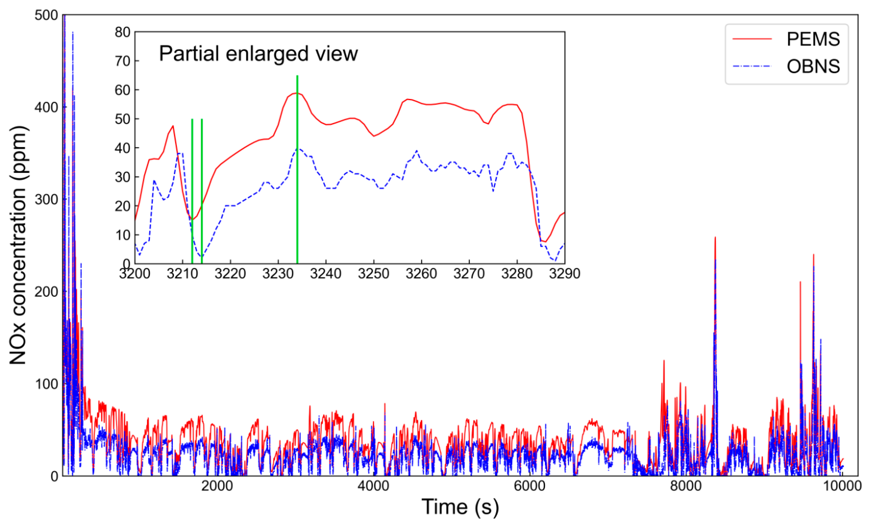
3.1. Analysis of the OBNS Measurement Characteristics

Figure 7 compares the transient measurement results of the OBNS and the PEMS in a test process. Figure 8 shows the cumulative relative error of the NOx mass emission calculated based on the OBNS and PEMS test data in 13 consecutive road tests. The calculation method for the cumulative relative error of NOx mass emission in a single test is as follows:

$${\epsilon }_M=\frac{\left|{\sum }_{i=1}^n{y}_{o,i}\ast -{\sum }_{i=1}^n{y}_{p,i}\right|}{{\sum }_{i=1}^n{y}_{p,i}}\ast 100$$

(5)

where ${\epsilon }_M$ represents the cumulative relative error of the NOx mass emission, $y_{o,i}$ represents the measured value of the OBNS at the i_th second, $y_{p,i}$ represents the PEMS test value at the i_th second, and n represents the number of the test data.

Figure 7 shows that compared to the PEMS emission analyser, the OBNS exhibited the following characteristics in practical operation. First, the average OBNS measurement deviation for the range of 0–50 ppm, 50–100 ppm, and 100 ppm was 12 ppm, 26 ppm, and 70 ppm, respectively. Second, the OBNS exhibited a response delay with an inconsistent time due to the complex and variable nature of actual exhaust environments. Figure 8 indicates that during 13 actual road driving tests, the cumulative relative error of the NOx mass emissions calculated through the OBNS compared to the PEMS tests exceeded 24%. Therefore, it is evident that the original OBNS measurement values are inadequate for accurately representing the actual NOx emissions.

3.2. Delay Correction for the OBNS Measurement

Table 5. Predictive performance of five classification algorithms.

Classification Algorithms	Average Cross-Validation Accuracy (%)	Training Time (s)
Decision tree	32.8	0.3
Naive Bayes	23.9	0.05
SVC	40.8	51.0
XGBoost	37.8	24.3
MLP	43.4	9.1

demonstrates the predictive performance of five classification algorithms on the measurement delay of the OBNS. It can be observed that the MLP algorithm exhibited significantly better performance in predicting the OBNS measurement delay compared to other classification algorithms. Although the decision tree and Naive Bayes algorithms had faster training processes, the classification accuracy was unsatisfactory. Compared to the SVC and XGBoost algorithms, a higher accuracy of 43.4% was achieved by the MLP algorithm, which also had the advantage of a shorter training time. Therefore, there is great practical value in predicting the OBNS measurement using the MLP classification algorithm.

Figure 9 presents the delay correction results of the OBNS measurement based on the MLP algorithm for the testing set. It can be observed that the measurement delay correction model based on the MLP algorithm exhibited superior correction effectiveness. The window proportion with a 0 s measurement delay increased from 11.8% to 45.6%, while the proportions of 2 s and 4 s decreased significantly. Consequently, the MLP algorithm was adopted to construct the measurement delay correction for the OBNS in the following research.

3.3. Correction of the Concentration Deviation for the OBNS Measurement

Table 6. OBNS measurement deviation correction based on different regression algorithms.

Regression Algorithms	MSE	R2	Training Time (s)
MLP	108.53	0.919	17.7
Decision tree	103.90	0.922	4.5
XGBoost	105.37	0.921	25.3
RFR	102.91	0.923	7.7

presents the computed results of the OBNS measurement deviation correction models based on different regression algorithms. The results show that all MLP, decision tree regression, XGBoost regression, and RFR exhibited good fitting effects, with an $R^2$ higher than 0.91. Among them, the RFR algorithm had the lowest MSE and the highest $R^2$. Moreover, in terms of the computation time, decision tree regression and RFR had relatively shorter computation times. Therefore, the RFR algorithm was selected to construct the OBNS measurement deviation correction model in this research.

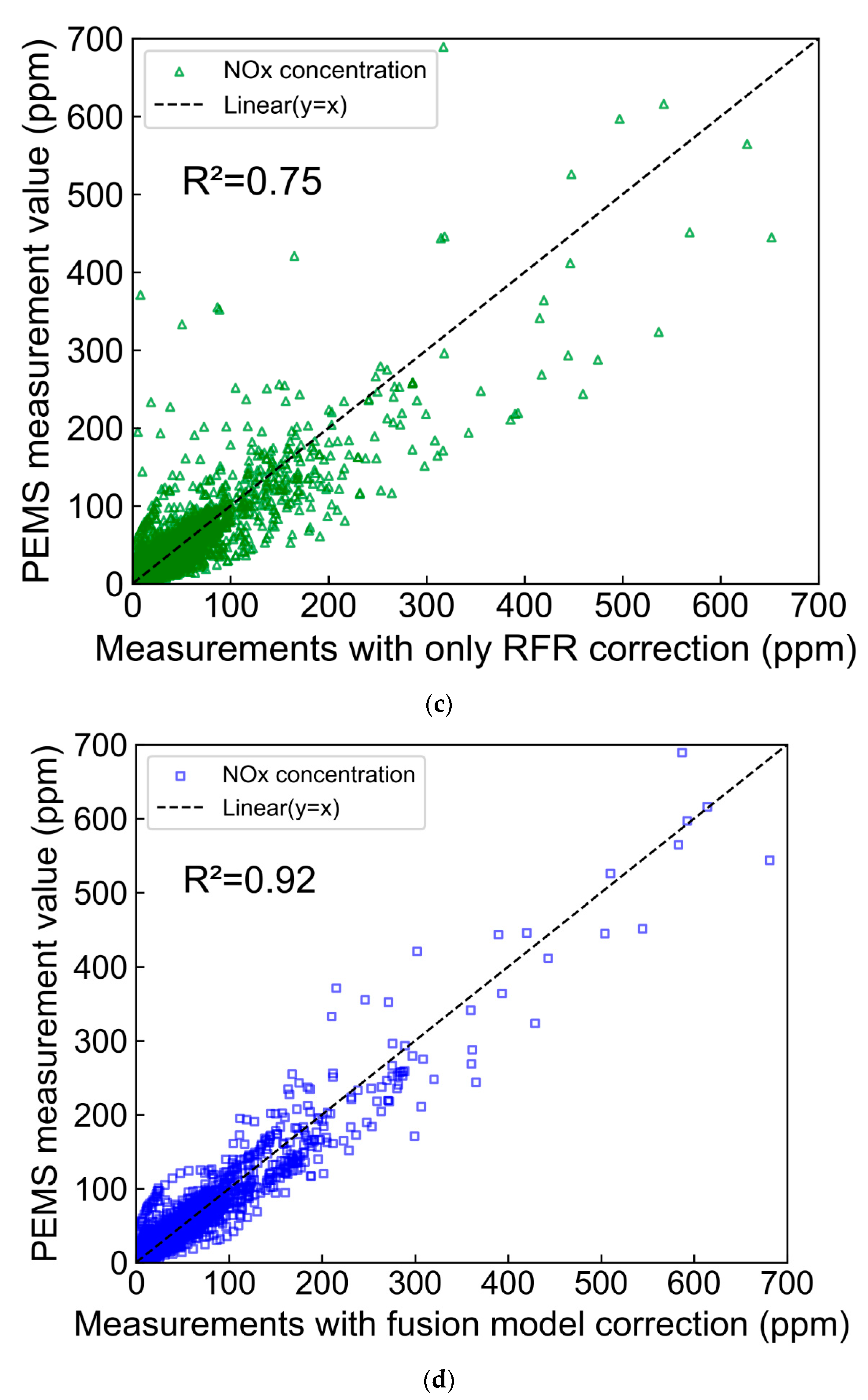
3.4. Evaluation of the MLP-RFR Fusion Algorithm Performance

Figure 10 compares the OBNS’s original measurement values, the PEMS test values, and the corrected OBNS concentration data based on the MLP-RFR fusion algorithm. Due to the extended duration of the experiment, the data curves were dense. Hence, the entire test process was divided into four parts according to the time sequence to facilitate the analysis of the fusion algorithm’s correction effectiveness. It can be seen that under most steady-state operating conditions, the deviation between the fusion algorithm’s corrected values and the PEMS test values was quite small. The correction effectiveness of the fusion algorithm was slightly worse only for a few peak operating points with significant emission variations. This can be attributed to poorer model fitting by insufficient data for such operating conditions in the training set. Firstly, when selecting the training dataset for the model, it was impossible to cover all the operating points of the diesel engine, negatively impacting the prediction accuracy. Secondly, there were subjective factors in the parameter selection and data processing. Third, there may have been some outliers in the experimental data, leading to prediction errors. In general, excellent correction performance for the OBNS measurement values can be seen in the MLP-RFR fusion algorithm.

Figure 11 and Figure 12 present the comparative results of the $R^2$ and MSE between the OBNS’s original measurement values, the corrected values using only MLP model, the corrected values using only the RFR model, the corrected values using the MLP-RFR fusion algorithm, and the PEMS test values. It can be seen that the MLP-RFR fusion algorithm exhibited a high goodness of fit for the OBNS signal. The $R^2$ moved from 0.56 to 0.92, while the MSE decreased from 586.72 to 109.42, obtaining a reduction of 81.3%. The results indicate that the MLP-RFR fusion algorithm can significantly improve the sensor’s measurement accuracy. It should also be noted that the RF algorithm without the MLP correction did not achieve satisfactory correction effectiveness for the OBNS measurement values. This demonstrates that the measurement delay correction forms the basis for correcting the measurement values of the OBNS.

Table 7. Measurement error performance of the OBNS and the fusion mode.

Type	Measurement Error
Corrected values using the MLP-RFR fusion algorithm	0–50 ppm: ±4.1 ppm (abs)
	50–100 ppm: ±6.1 ppm (abs) 50–100 ppm: ±9.3% (rel.)
	100–150 ppm: ±27.2 ppm (abs) 100–150 ppm: ±22.4% (rel.)
	150–200 ppm: ±30.6 ppm (abs) 150–200 ppm: ±18.1% (rel.)
	200–300 ppm: ±41.1 ppm (abs) 200–300 ppm: ±17.5% (rel.)
	>300 ppm: ±72.0 ppm (abs) >300 ppm: ±15.9% (rel.)
OBNS original measurement values	0–50 ppm: ±12.1 ppm (abs)
	50–100 ppm: ±25.6 ppm (abs) 50–100 ppm: ±41.5% (rel.)
	100–150 ppm: ±42.8 ppm (abs) 100–150 ppm: ±34.9% (rel.)
	150–200 ppm: ±63.6 ppm (abs) 150–200 ppm: ±37.0% (rel.)
	200–300 ppm: ±89.0 ppm (abs) 200–300 ppm: ±37.4% (rel.)
	>300 ppm: ±214.4 ppm (abs) >300 ppm: ±45.5% (rel.)

presents the measurement error performance of the OBNS and the fusion model on the test set. It can be seen that after incorporating the MLP-RFR fusion algorithm correction, the measurement error was significantly reduced, particularly in the low NOx concentration range (<90 ppm). The relevant error decreased from ±15 ppm to ±4 ppm, obtaining a reduction of 73.3%. In the high NOx concentration range (91–1000 ppm), the relative measurement error decreased from 35% to 17%, which was not strong as the low NOx concentration range. This is mainly due to the relatively limited high NOx concentration data in the training set, which hindered the fusion model from achieving outstanding learning effects.

4. Conclusions and Future Work

To address the issue of the low measurement accuracy of the OBNS, this research constructed a machine learning model based on the MLP-RFR fusion of classification and regression algorithms for the real-time signal correction of the OBNS. The findings of this research could significantly help to achieve the effective remote monitoring of emissions from heavy-duty diesel vehicles. The main conclusions of this research can be drawn as follows:

(1) Delay identification models for the OBNS measurement and deviation correction models for concentration were constructed based on different classification and regression algorithms, respectively. The computation results demonstrate that the delay identification model based on the multilayer perceptron algorithm achieved the highest prediction accuracy, while the deviation correction model based on the random forest regression algorithm performed the best.

(2) The measurement accuracy of the OBNS was significantly improved by the MLP-RFR fusion model. In the concentration range of 0–90 ppm, the absolute measurement error of the sensor decreased from ±15 ppm to ±4 ppm, resulting in a 73.3% reduction in measurement error. In the concentration range of 91–1000 ppm, the relative measurement error of the sensor decreased from 35% to 17%.

In this study, measurement errors of the vehicle-mounted NOx sensors were successfully corrected using machine learning algorithms, and promising results were achieved. However, certain limitations that offer valuable insights for further development and improvement of the model must be acknowledged. For instance, the training data primarily originated from the low concentration range of NOx data (<90 ppm) when the emission state of the test vehicle was relatively favourable. As a consequence, good performance in correcting low-concentration NOx data was demonstrated by the model. Nevertheless, when higher concentrations of NOx data were confronted, the correction effectiveness of the model decreased due to inadequate representation in the training data. This limitation can potentially impact the accuracy and stability of high-concentration NOx data correction in real-world applications, thereby necessitating further research and refinement.

Furthermore, consideration should also be given to the possibility that other factors, such as sensor ageing and variations in the environmental temperature, may influence the corrected measurement data in practical applications. Hence, future research efforts could address these issues and comprehensively consider various interfering factors and alternative algorithm choices to achieve a more precise and reliable NOx data correction method.

References

1. Li, X.; Ai, Y.; Ge, Y.; Qi, J.; Feng, Q.; Hu, J.; Porter, W.C.; Miao, Y.; Mao, H.; Jin, T. Integrated effects of SCR, velocity, and Air-fuel Ratio on gaseous pollutants and CO2 emissions from China V and VI heavy-duty diesel vehicles. Sci. Total Environ. 2022, 811, 152311. [Google Scholar] [CrossRef] [PubMed]
2. Zhang, X.; Li, J.; Liu, H.; Li, Y.; Li, T.; Sun, K.; Wang, T. A fuel-consumption based window method for PEMS NOx emission calculation of heavy-duty diesel vehicles: Method description and case demonstration. J. Environ. Manag. 2023, 325, 116446. [Google Scholar] [CrossRef] [PubMed]
3. Wang, Y.; Yin, H.; Wang, J.; Hao, C.; Xu, X.; Wang, Y.; Yang, Z.; Hao, L.; Tan, J.; Wang, X.; et al. China 6 moving average window method for real driving emission evaluation: Challenges, causes, and impacts. J. Environ. Manag. 2022, 319, 115737. [Google Scholar] [CrossRef]
4. Sharp, C.A.; Feist, M.D.; Laroo, C.A.; Spears, M.W. Determination of PEMS Measurement Allowances for Gaseous Emissions Regulated Under the Heavy-Duty Diesel Engine In-Use Testing Program: Part 3—Results and Validation. SAE Int. J. Fuels Lubr. 2009, 2, 407–421. [Google Scholar] [CrossRef]
5. Zheng, X.; Wu, Y.; Zhang, S.; Hu, J.; Zhang, K.M.; Li, Z.; He, L.; Hao, J. Characterizing particulate polycyclic aromatic hydrocarbon emissions from diesel vehicles using a portable emissions measurement system. Sci. Rep. 2017, 7, 10058. [Google Scholar] [CrossRef]
6. Mądziel, M. Liquefied Petroleum Gas-Fuelled Vehicle CO2 Emission Modelling Based on Portable Emission Measurement System, On-Board Diagnostics Data, and Gradient-Boosting Machine Learning. Energies 2023, 16, 2754. [Google Scholar] [CrossRef]
7. Jaworski, A.; Lejda, K.; Mądziel, M.; Ustrzycki, A. Assessment of the emission of harmful car exhaust components in real traffic conditions. IOP Conf. Ser. Mater. Sci. Eng. 2018, 421, 042031. [Google Scholar] [CrossRef]
8. Cheng, Y.; He, L.; He, W.; Zhao, P.; Wang, P.; Zhao, J.; Zhang, K.; Zhang, S. Evaluating on-board sensing-based nitrogen oxides (NOX) emissions from a heavy-duty diesel truck in China. Atmos. Environ. 2019, 216, 116908. [Google Scholar] [CrossRef]
9. Zhang, S.; Wu, Y.; Hu, J.; Huang, R.; Zhou, Y.; Bao, X.; Fu, L.; Hao, J. Can Euro V Heavy-Duty Diesel Engines, Diesel Hybrid and Alternative Fuel Technologies Mitigate NOX Emissions? New Evidence from On-Road Tests of Buses in China. Appl. Energy 2014, 132, 118–126. [Google Scholar] [CrossRef]
10. Zhang, S.; Zhao, P.; He, L.; Yang, Y.; Liu, B.; He, W.; Cheng, Y.; Liu, Y.; Liu, S.; Hu, Q.; et al. On-board monitoring (OBM) for heavy-duty vehicle emissions in China: Regulations, early-stage evaluation, and policy recommendations. Sci. Total Environ. 2020, 731, 139045. [Google Scholar] [CrossRef]
11. Hofmann, L.; Rusch, K.; Fischer, S.; Lemire, B. Onboard Emissions Monitoring on a HD Truck with an SCR System Using Nox Sensors; SAE Transactions; SAE International: Warrendale, PA, USA, 2004; pp. 559–572. [Google Scholar] [CrossRef]
12. Giampà, A.; Petri, E.; Saponara, S.; Terreni, P. Sensor Modeling and Fusion Algorithms for NOx Measures towards Zero Emissions Vehicles. In Proceedings of the 2009 IEEE International Workshop on Robotic and Sensors Environments, Lecco, Italy, 6–7 November 2009; IEEE: Piscataway, NJ, USA, 2009; pp. 151–156. [Google Scholar]
13. Fischer, S.; Pohle, R.; Farber, B.; Proch, R.; Kaniuk, J.; Fleischer, M.; Moos, R. Method for Detection of NOx in Exhaust Gases by Pulsed Discharge Measurements Using Standard Zir-conia-Based Lambda Sensors. Sens. Actuators B Chem. 2010, 147, 780–785. [Google Scholar] [CrossRef]
14. Wang, Y.-Y.; Zhang, H.; Wang, J. NOx Sensor Reading Correction in Diesel Engine Selective Catalytic Reduction System Applications. IEEE/ASME Trans. Mechatron. 2016, 21, 460–471. [Google Scholar] [CrossRef]
15. Liu, F.; Guan, Y.; Dai, M.; Zhang, H.; Guan, Y.; Sun, R.; Liang, X.; Sun, P.; Liu, F.; Lu, G. High-Performance Mixed-Potential Type NO2 Sensors Based on Three-Dimensional TPB and Co3V2O8 Sensing Electrode. Sens. Actuators B Chem. 2015, 216, 121–127. [Google Scholar] [CrossRef]
16. Bhardwaj, A.; Bae, H.; Namgung, Y.; Lim, J.; Song, S.J. Influence of sintering temperature on the physical, electrochemical and sensing properties of α-Fe2O3-SnO2 nanocomposite sensing electrode for a mixed-potential type NOx sensor. Ceram. Int. 2019, 45, 2309–2318. [Google Scholar] [CrossRef]
17. Huang, A.; Lyu, Y.; Guo, Z.; Zhao, X. A Temperature and Humidity Compensation Method for On-Board NOx Sensors with LSTM Network. In Proceedings of the 2020 International Conference on Sensing, Measurement & Data Analytics in the Era of Artificial Intelligence (ICSMD), Xi’an, China, 15–17 October 2020; IEEE: Piscataway, NJ, USA, 2020. [Google Scholar] [CrossRef]
18. Li, P.; Lü, L. Research on a China 6b heavy-duty diesel vehicle real-world engine out NOx emission deterioration and ambient correction using big data approach. Environ. Sci. Pollut. Res. 2022, 29, 6949–6976. [Google Scholar] [CrossRef]
19. Flores Fernández, A.; Sánchez Morales, E.; Botsch, M.; Facchi, C.; García Higuera, A. Generation of Correction Data for Autonomous Driving by Means of Machine Learning and On-Board Diagnostics. Sensors 2023, 23, 159. [Google Scholar] [CrossRef]
20. Chastko, K.; Adams, M. Assessing the accuracy of long-term air pollution estimates produced with temporally adjusted short-term observations from unstructured sampling. J. Environ. Manag. 2019, 240, 249–258. [Google Scholar] [CrossRef]
21. Just, A.C.; De Carli, M.M.; Shtein, A.; Dorman, M.; Lyapustin, A.; Kloog, I. Correcting Measurement Error in Satellite Aerosol Optical Depth with Machine Learning for Modeling PM2.5 in the Northeastern USA. Remote Sens. 2018, 10, 803. [Google Scholar] [CrossRef]
22. Kim, Y.-H.; Ha, J.-H.; Yoon, Y.; Kim, N.-Y.; Im, H.-H.; Sim, S.; Choi, R.K.Y. Improved Correction of Atmospheric Pressure Data Obtained by Smartphones through Machine Learning. Comput. Intell. Neurosci. 2016, 2016, 9467878. [Google Scholar] [CrossRef]
23. Lee, W.M. Getting Started with Scikit-Learn for Machine Learning. In Python® Machine Learning; John Wiley & Sons, Inc.: Hoboken, NJ, USA, 2019; pp. 93–117. [Google Scholar] [CrossRef]
24. Yin, Y.; Jang-Jaccard, J.; Xu, W.; Singh, A.; Zhu, J.; Sabrina, F.; Kwak, J. IGRF-RFE: A Hybrid Feature Selection Method for MLP-Based Network Intrusion De-tection on UNSW-NB15 Dataset. J. Big Data 2023, 10, 15. [Google Scholar] [CrossRef]
25. Anushiya, R.; Lavanya, V. A new deep-learning with swarm based feature selection for intelligent intrusion detection for the Internet of things. Meas. Sens. 2023, 26, 100700. [Google Scholar] [CrossRef]
26. Bakro, M.; Kumar, R.R.; Alabrah, A.; Ashraf, Z.; Ahmed, M.N.; Shameem, M.; Abdelsalam, A. An Improved Design for a Cloud Intrusion Detection System Using Hybrid Features Selection Approach with ML Classifier; IEEE Access: Piscataway, NJ, USA, 2023. [Google Scholar]
27. Taud, H.; Mas, J.F. Multilayer Perceptron (MLP). In Geomatic Approaches for Modeling Land Change Scenarios; Springer: Berlin/Heidelberg, Germany, 2018; pp. 451–455. [Google Scholar]
28. Wong, T.-T. Performance evaluation of classification algorithms by k-fold and leave-one-out cross validation. Pattern Recognit. 2015, 48, 2839–2846. [Google Scholar] [CrossRef]
29. Srivastava, N.; Hinton, G.; Krizhevsky, A.; Sutskever, I.; Salakhutdinov, R. Dropout: A Simple Way to Prevent Neural Networks from Overfitting. J. Mach. Learn. Res. 2014, 15, 1929–1958. [Google Scholar]
30. Syarif, I.; Prugel-Bennett, A.; Wills, G. SVM Parameter Optimization using Grid Search and Genetic Algorithm to Improve Classification Performance. TELKOMNIKA (Telecommun. Comput. Electron. Control) 2016, 14, 1502. [Google Scholar] [CrossRef]
Figure 1. Flowchart of the research approach.
Energies 16 06082 g001
Figure 2. Diagram of measurement points for the OBNS and PEMS.
Energies 16 06082 g002
Figure 3. MLP-RFR fusion correction model for correcting the OBNS.
Energies 16 06082 g003
Figure 4. Data extraction of the sliding window with different lag times.
Energies 16 06082 g004
Figure 5. Structure of the RF algorithm.
Energies 16 06082 g005
Figure 6. Structure of the MLP algorithm.
Energies 16 06082 g006
Figure 7. Comparison of the transient measurement results between the OBNS and the PEMS.
Energies 16 06082 g007
Figure 8. Cumulative relative error of the NOx mass emissions based on the OBNS and PEMS test data.
Energies 16 06082 g008
Figure 9. The delay correction results of the OBNS measurement based on the MLP algorithm.
Energies 16 06082 g009
Figure 10. Comparison of the NOx emissions between the original OBNS, the PEMS, and the corrected OBNS (MLP-RFR).
Energies 16 06082 g010
Figure 11. Comparison of the R 2 between the original, different model corrections, and PEMS. (a) OBNS original measurement; (b) only MLP correction; (c) only RFR correction; (d) with MLP-RFR fusion algorithm.
Energies 16 06082 g011aEnergies 16 06082 g011b
Figure 12. Comparison of the MSE between the original, different model corrections, and PEMS.
Energies 16 06082 g012