
Random Forest Model of Flow Pattern Identification in Scavenge Pipe Based on EEMD and Hilbert Transform

Abstract
:1. Introduction
2. Theoretical Basis
2.1. EEMD
- (1)
- Set the overall average number of times M;
- (2)
- Add a white noise with standard normal distribution to the original signal to produce a new signal: , where denotes the mth addition of white noise sequence, denotes the signal with the ith additional noise, m = 1, 2…M;
- (3)
- EMD decomposition is performed separately for the resulting noise-containing signals, and the respective sums are obtained in the form:where, is the nth IMF obtained by decomposition after m additions of white noise, is the residual function, representing the average trend of the signal, and n is the number of IMFs;
- (4)
- Repeat step (2) and step (3) for M times, and each decomposition adds white noise signals with different amplitudes to obtain the set of IMFs as:
- (5)
- Using the principle that the statistical mean of uncorrelated sequences is zero, the above corresponding IMFs are subjected to a pooled averaging operation to obtain the final IMF after EEMD decomposition:where is the nth IMF of the EEMD decomposition, , , and the residual component is the difference between the original data and j IMFs. The final decomposition form of the signal is obtained:
2.2. Hilbert Transform
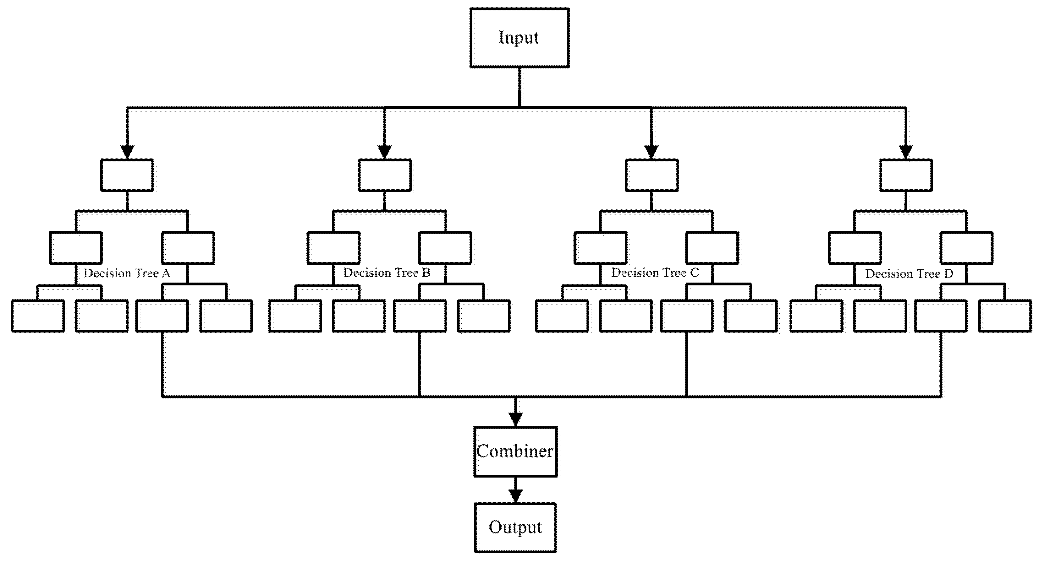
2.3. Random Forest
- (1)
- Randomly select a portion of data and features from the original data to construct a decision tree.
- (2)
- Repeat n times to construct n decision trees.
- (3)
- For each new data point, pass it into each tree for classification and get the classification result for each tree.
- (4)
- Each new data point is classified as the most classified result of the random forest.
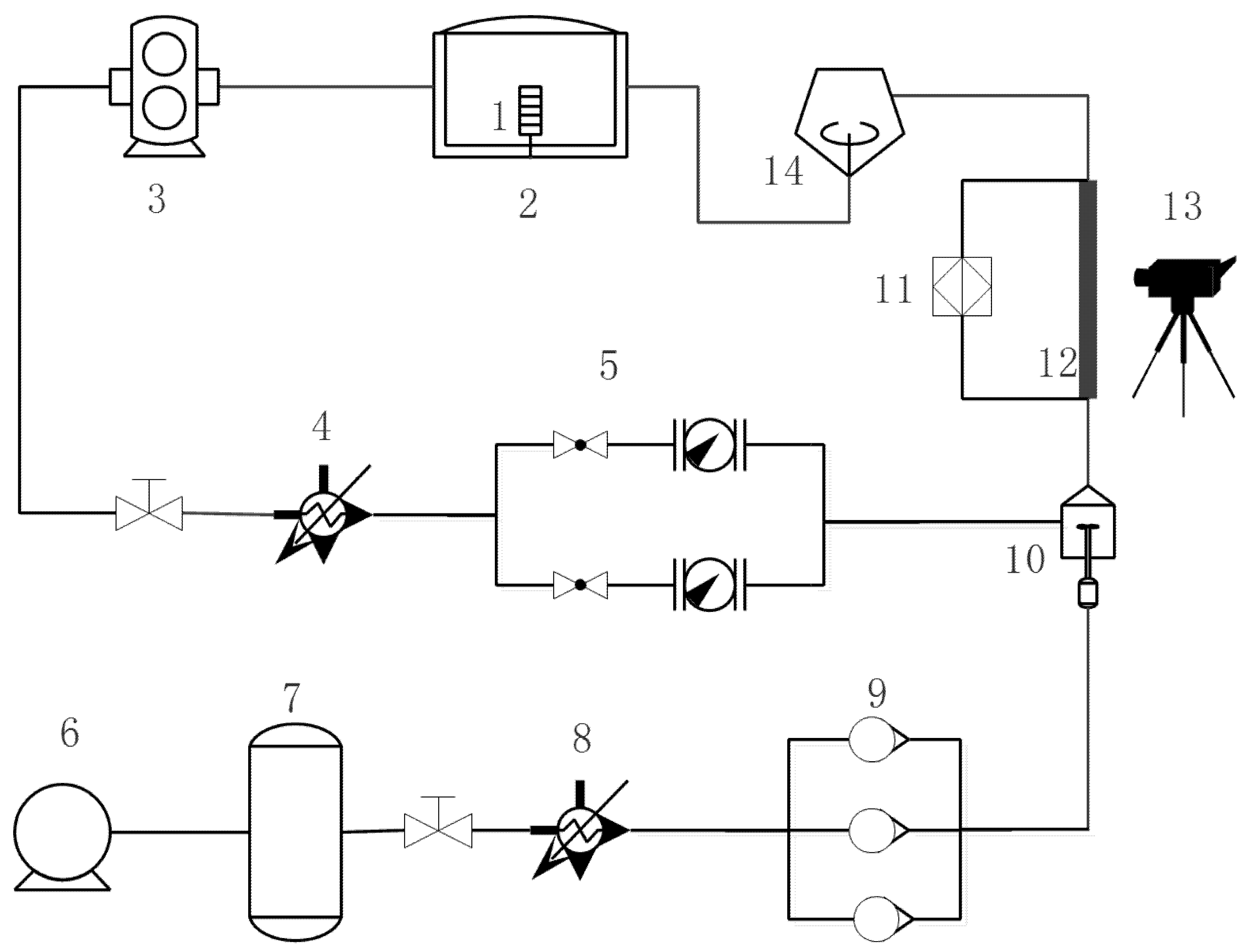
3. Experimental Apparatus
4. Results and Discussion
4.1. Experimental Study on Oil Gas Two-Phase Flow in Scavenge Pipe
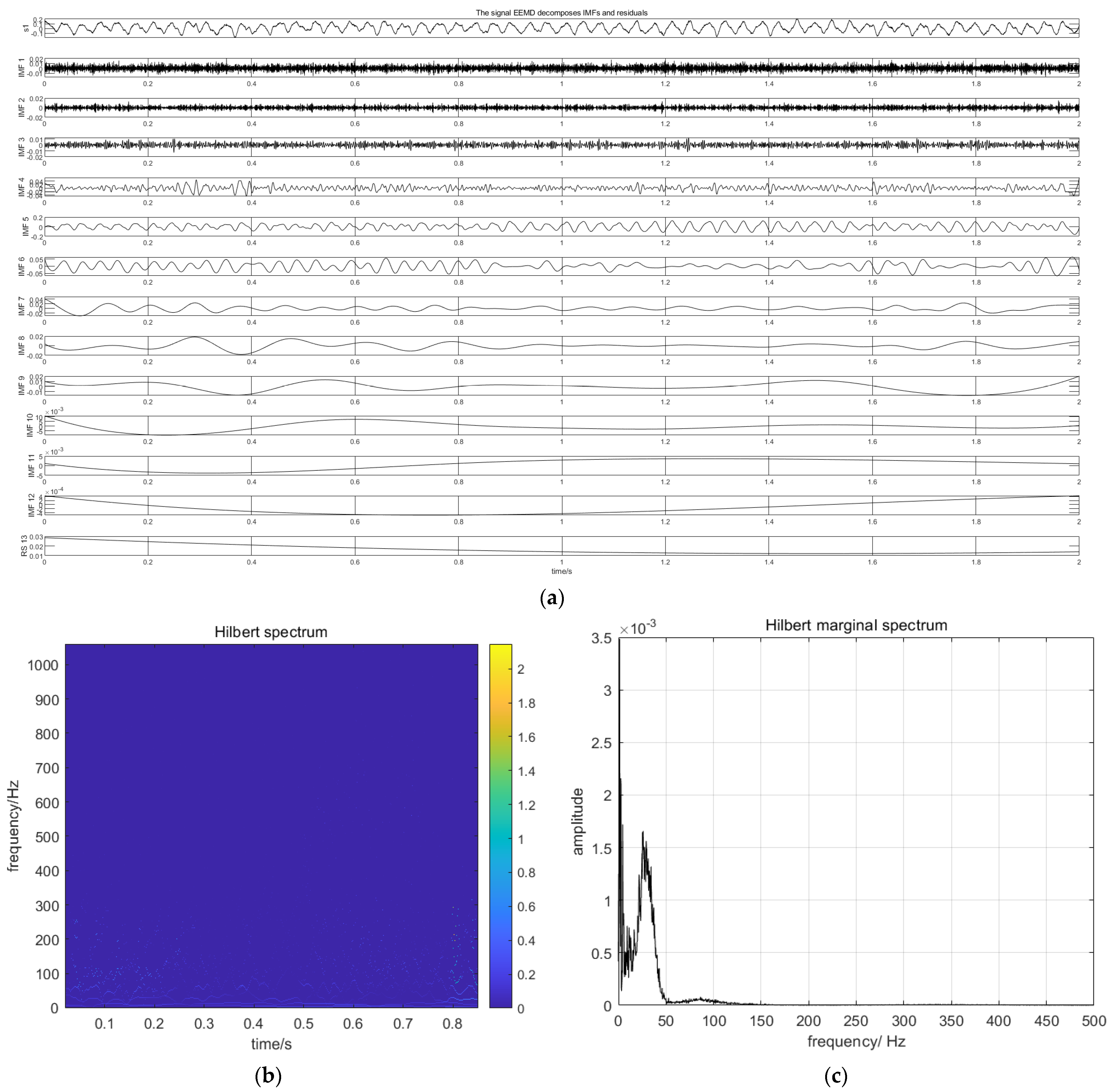
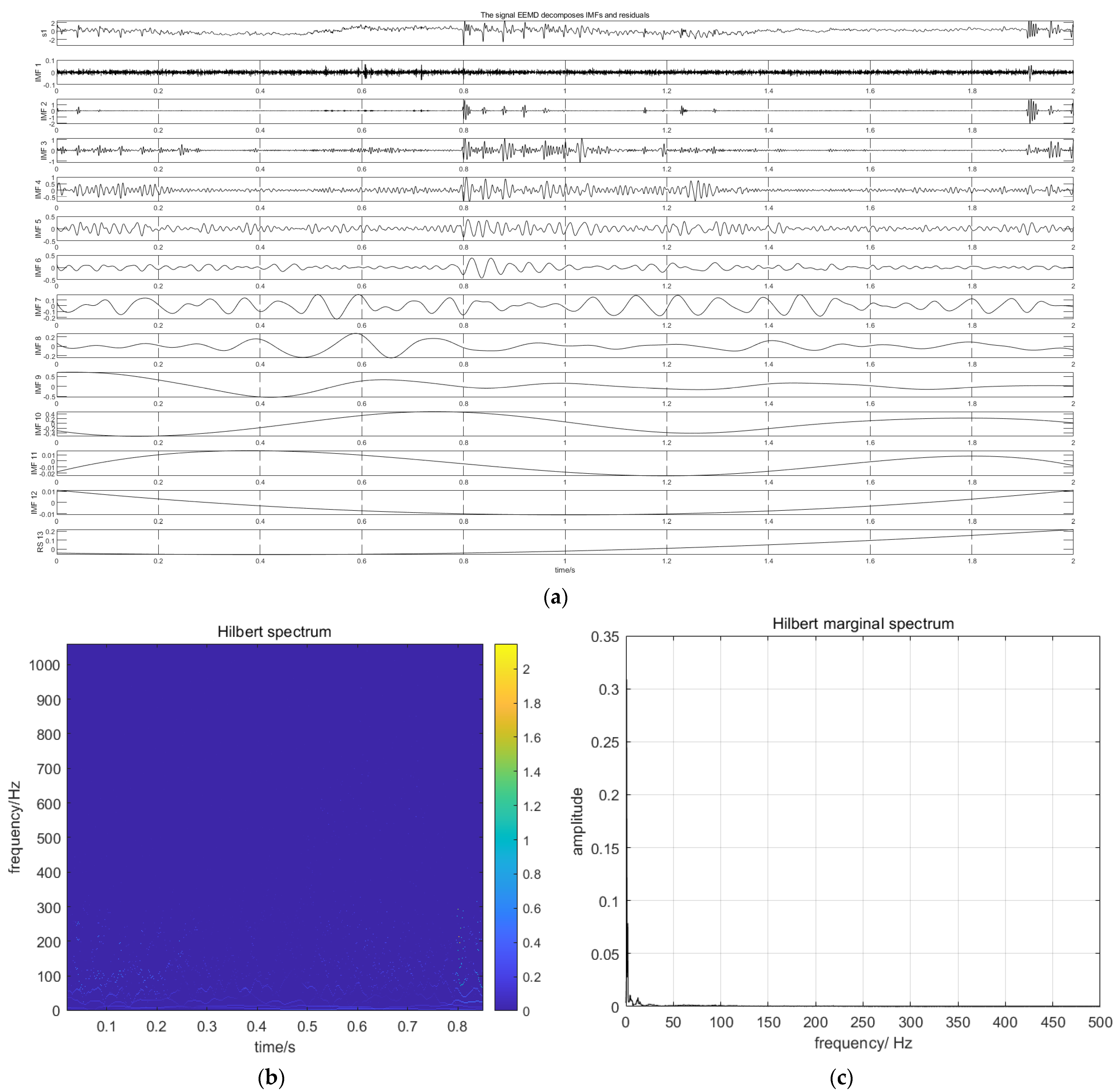
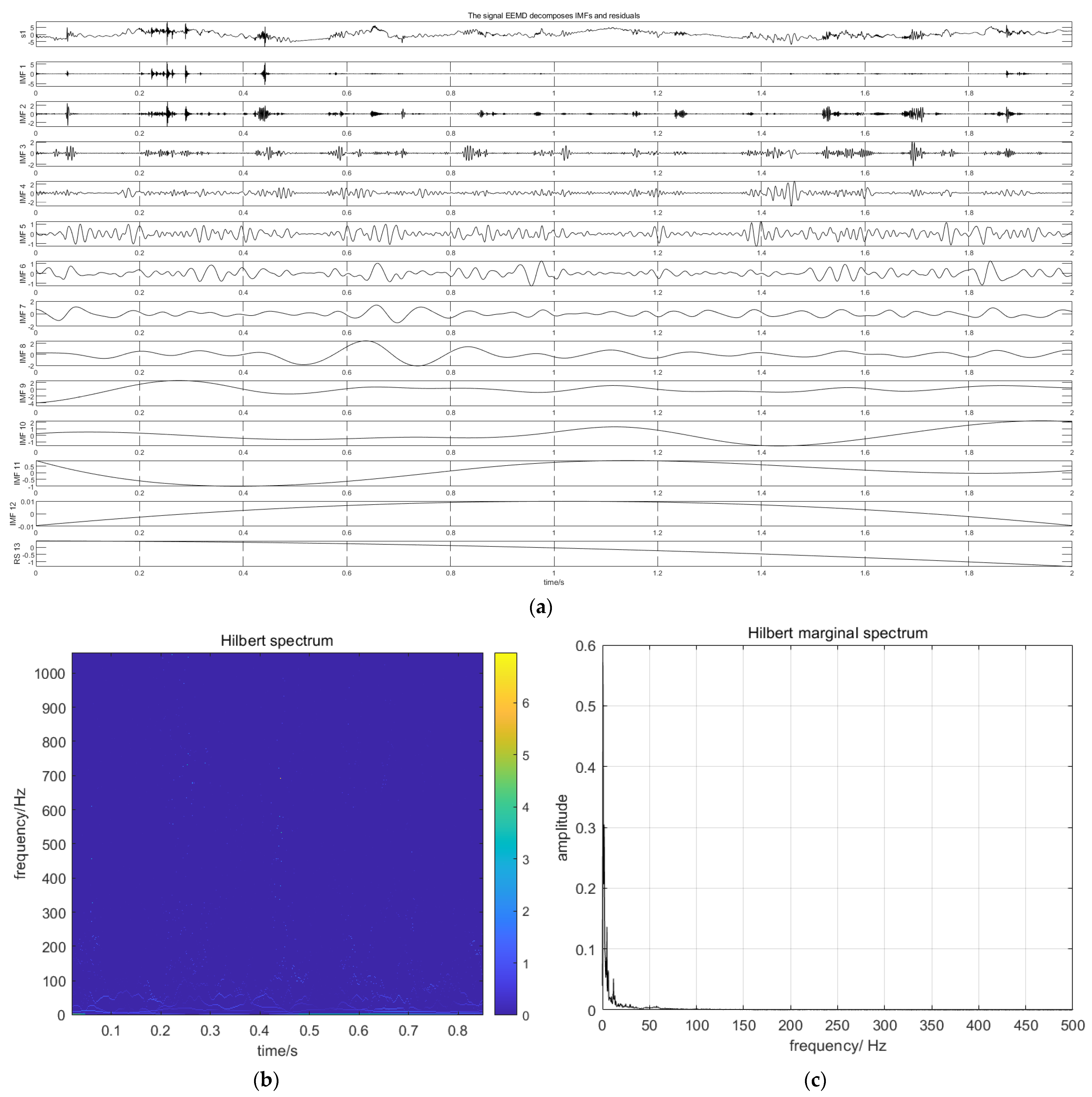
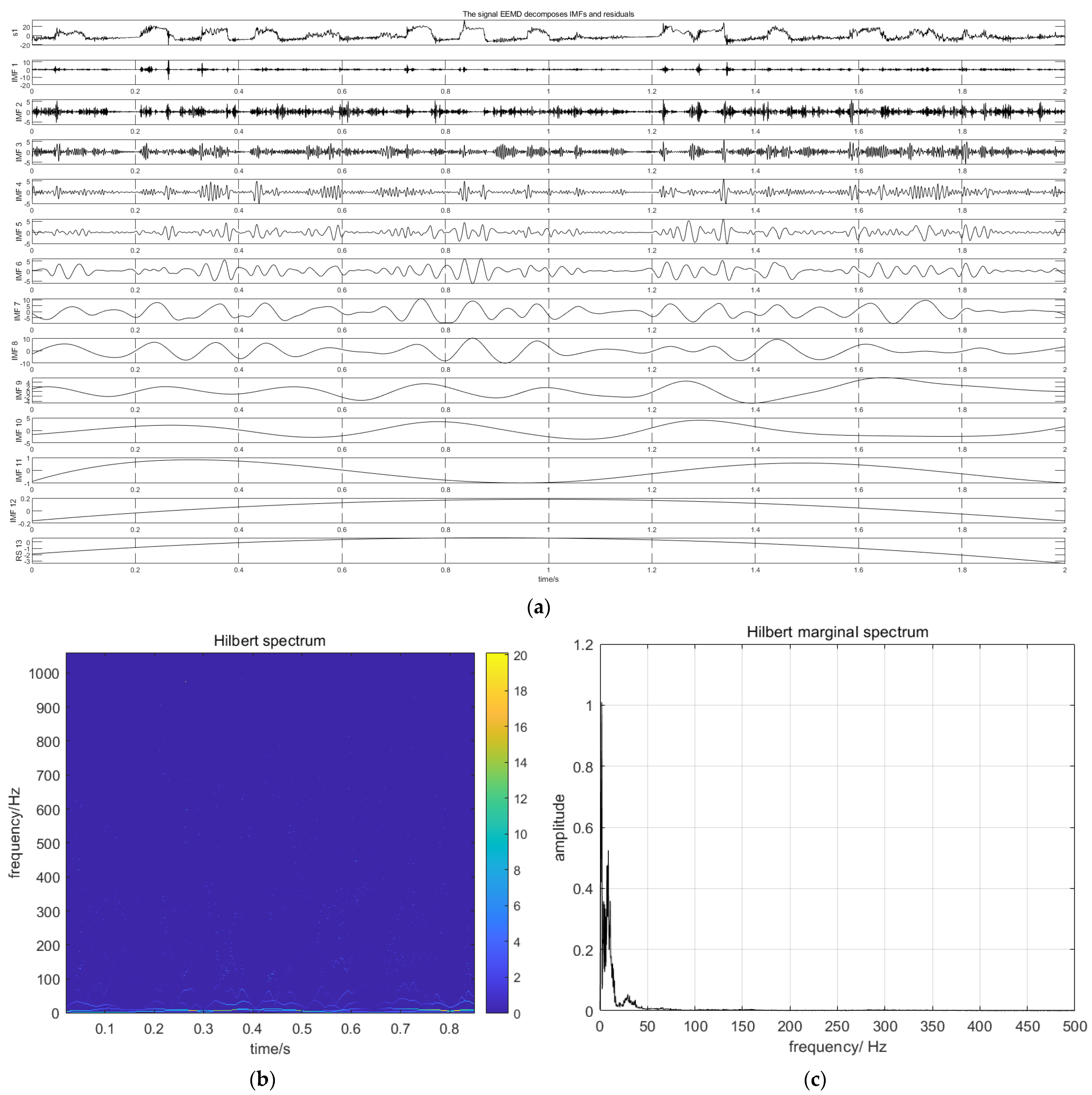
4.2. Decomposing the Pressure Signal of Oil Gas Two-Phase Flow in the Scavenge Pipe
4.3. Establishing Flow Pattern Recognition Model
5. Conclusions
Author Contributions
Funding
Data Availability Statement
Conflicts of Interest
References
- Li, G.Q. Present and future of aeroengine oil system. Aeroengine 2011, 6, 49–52. [Google Scholar]
- Flouros, M.; Iatrou, G.; Yakinthos, K.; Cottier, F.; Hirschmann, M. Two-Phase Flow Heat Transfer and Pressure Drop in Horizontal Scavenge Pipes in an Aero-engine. J. Eng. Gas Turbines Power 2015, 137, 081901. [Google Scholar] [CrossRef]
- Chandra, B.; Simmons, K.; Pickering, S.; Collicott, S.H.; Wiedemann, N. Study of gas/liquid behavior within an aero enginebearing chamber. J. Eng. Gas Turbines Power 2013, 135, 051201. [Google Scholar] [CrossRef]
- Figueiredo, M.M.F.; Goncalves, J.L.; Nakashima, A.M.V.; Fileti, A.M.; Carvalho, R.; Carvalho, R. The use of an ultrasonic technique and neural networks for the identification of the flow pattern and measurement of the gas volume fraction in multiphase flows. Exp. Therm. Fluid Sci. 2016, 70, 29. [Google Scholar] [CrossRef]
- Merchan, F.; Guerra, A.; Poveda, H.; Guzmán, H.M.; Sanchez-Galan, J.E. Bioacoustic Classification of Antillean Manatee Vocalization Spectrograms Using Deep Convolutional Neural Networks. Appl. Sci. 2020, 10, 3286. [Google Scholar] [CrossRef]
- Ong, C.L.; Thome, J.R. Macro-to-microchannel transition in two-phase flow: Part 1—Two-phase flow patterns and film thickness measurements. Exp. Therm. Fluid Sci. 2011, 35, 37–47. [Google Scholar] [CrossRef]
- Rafalko, G.; Mosdorf, R.; Gorski, G. Two-phase flow pattern identification in minichannels using image correlation analysis. Int. Commun. Heat Mass Transf. 2020, 113, 104508.1–104508.9. [Google Scholar] [CrossRef]
- Thaker, J.; Banerjee, J. Characterization of two-phase slug flow sub-regimes using flow visualization. J. Pet. Sci. Eng. 2015, 135, 561–576. [Google Scholar] [CrossRef]
- Sizikov, V.S.; Dovgan, A.N.; Tsepeleva, A.D. Restoration of nonuniformly smeared images. J. Opt. Technol. 2020, 87, 110–116. [Google Scholar] [CrossRef]
- Nguyen, V.T.; Dong, J.E.; Song, C.H. An application of the wavelet analysis technique for the objective discrimination of two-phase flow patterns. Int. J. Multiph. Flow 2010, 36, 755–768. [Google Scholar] [CrossRef]
- De Giorgi, M.G.; Ficarella, A.; Lay-Ekuakille, A. Monitoring Cavitation Regime from Pressure and Optical Sensors: Comparing Methods Using Wavelet Decomposition for Signal Processing. IEEE Sens. J. 2015, 15, 4684–4691. [Google Scholar] [CrossRef]
- Dong, F.; Zhang, S.; Shi, X.; Wu, H.; Tan, C. Flow Regimes Identification-based Multidomain Features for Gas–Liquid Two-Phase Flow in Horizontal Pipe. IEEE Trans. Instrum. Meas. 2021, 99, 1–11. [Google Scholar] [CrossRef]
- Ji, H.; Long, J.; Fu, Y.; Huang, Z.; Wang, B.; Li, H. Flow Pattern Identification Based on EMD and LS-SVM for Gas–Liquid Two-Phase Flow in a Minichannel. IEEE Trans. Instrum. Meas. 2011, 60, 1917–1924. [Google Scholar]
- Ding, H.; Huang, Z.; Song, Z.; Yan, Y. Hilbert–Huang transform-based signal analysis for the characterization of gas–liquid two-phase flow. Flow Meas. Instrum. 2007, 18, 37–46. [Google Scholar] [CrossRef]
- Huang, N.E.; Shen, Z.; Long, S.R.; Wu, M.C.; Shih, H.H.; Zheng, Q.; Yen, N.; Tung, C.; Liu, H.H. The empirical mode decomposition and the Hilbert spectrum for nonlinear and non-stationary time series analysis. Proc. Math. Phys. Eng. Sci. 1998, 454, 903–995. [Google Scholar] [CrossRef]
- Dliou, A.; Latif, R.; Laaboubi, M.; Maoulainine, F.; Elouaham, S. Time-frequency analysis of a noised ECG signals using empirical mode decomposition and Choi-Williams techniques. Int. J. Syst. Control. Commun. 2013, 5, 231–245. [Google Scholar] [CrossRef]
- Wu, Z.; Huang, N.E. Ensemble empirical mode decomposition: A noise-assisted data analysis method. Adv. Adapt. Data Anal. 2011, 1, 1–41. [Google Scholar] [CrossRef]
- Chu, W.; Liu, Y.; Zhu, H.; Yang, X.; Pan, L. Application of EEMD-Multiscale Entropy Algorithm in the Signal Analysis of Narrow Channel Two-Phase Flow Under Rolling Motion. In Proceedings of the International Conference on Nuclear Engineering, Virtual, 4–6 August 2021; American Society of Mechanical Engineers: New York, NY, USA, 2021; Volume 85246, p. V001T04A001. [Google Scholar]
- Chen, Z.; Liu, B.; Yan, X.; Yang, H. An Improved Signal Processing Approach Based on Analysis Mode Decomposition and Empirical Mode Decomposition. Energies 2019, 12, 3077. [Google Scholar] [CrossRef]
- Kurbatskii, V.G.; Sidorov, D.N.; Spiryaev, V.A.; Tomin, N. On the neural network approach for forecasting of nonstationary time series on the basis of the Hilbert-Huang transform. Autom. Remote Control 2011, 72, 1405–1414. [Google Scholar] [CrossRef]
- Levin, A.A.; Tairov, E.A.; Spiryaev, V.A. Self-excited pressure pulsations in ethanol under heater subcooling. Thermophys. Aeromechanics 2017, 24, 61–71. [Google Scholar] [CrossRef]
- Behrends, H.; Millinger, D.; Weihs-Sedivy, W.; Javornik, A.; Roolfs, G.; Geißendörfer, S. Analysis of Residual Current Flows in Inverter Based Energy Systems Using Machine Learning Approaches. Energies 2022, 15, 582. [Google Scholar] [CrossRef]
- Zhang, Y.; Azman, A.N.; Xu, K.; Kang, C.; Kim, H.-B. Two-phase flow regime identification based on the liquid-phase velocity information and machine learning. Exp. Fluids 2020, 61, 212. [Google Scholar] [CrossRef]
- Yadav, B.; Devi, V.S. Novelty detection applied to the classification problem using Probabilistic Neural Network. In Proceedings of the Computational Intelligence & Data Mining, Bhubaneswar, India, 5–6 December 2015; IEEE: New York, NY, USA, 2015. [Google Scholar] [CrossRef]
- Liu, L.; Bai, B. Flow regime identification of swirling gas-liquid flow with image processing technique and neural networks. Chem. Eng. Sci. 2019, 199, 588–601. [Google Scholar] [CrossRef]
- Charbuty, B.; Abdulazeez, A. Classification Based on Decision Tree Algorithm for Machine Learning. J. Appl. Sci. Technol. Trends 2021, 2, 20–28. [Google Scholar] [CrossRef]
- Kawahara, A.; Sadatomi, M.; Nei, K.; Matsuo, H. Experimental study on bubble velocity, void fraction and pressure drop for gas–liquid two-phase flow in a circular microchannel. Int. J. Heat Fluid Flow 2009, 30, 831–841. [Google Scholar] [CrossRef]
- Hanafizadeh, P.; Saidi, M.; Gheimasi, A.N.; Ghanbarzadeh, S. Experimental investigation of air–water, two-phase flow regimes in vertical mini pipe. Sci. Iran. 2011, 18, 923–929. [Google Scholar] [CrossRef]


| Physical Properties | Air | Oil |
|---|---|---|
| ρ (kg/s) | 1.225 | 1003.5 |
| µ (kg/m·s) | 1.84 × 10⁻⁵ | 0.0051 |
| Cp (J/kg·K) | 1006.43 | 1880 |
| λ (W/m·K) | 0.0242 | 0.12 |
| Order Number | Gas Reduced Velocity (m/s) | Flow Pattern | Flow Patterns Photos |
|---|---|---|---|
| 1 | 0 | pure fluid |  |
| 2 | 0.042 | bubble flow |  |
| 3 | 0.084 | plug flow |  |
| 4 | 0.127 | plug flow | 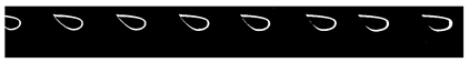 |
| 5 | 0.169 | plug flow |  |
| 6 | 0.212 | plug flow |  |
| 7 | 0.254 | slug flow | 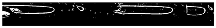 |
| 8 | 0.297 | slug flow |  |
| 9 | 0.339 | slug flow | 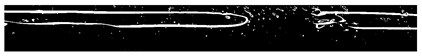 |
| 10 | 0.382 | slug flow |  |
| 11 | 0.424 | slug flow |  |
| 12 | 0.636 | slug flow | 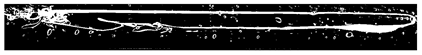 |
| 13 | 0.849 | slug flow | 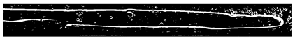 |
| 14 | 1.061 | slug flow |  |
| 15 | 1.273 | slug flow | 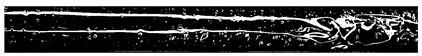 |
| 16 | 1.698 | annular flow |  |
| 17 | 2.123 | annular flow | 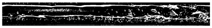 |
| Flow Pattern | Pure Liquid | Bubble Flow | Plug Flow | Slug Flow | Annular Flow |
|---|---|---|---|---|---|
| Coding | 1 | 2 | 3 | 4 | 5 |
Disclaimer/Publisher’s Note: The statements, opinions and data contained in all publications are solely those of the individual author(s) and contributor(s) and not of MDPI and/or the editor(s). MDPI and/or the editor(s) disclaim responsibility for any injury to people or property resulting from any ideas, methods, instructions or products referred to in the content. |
© 2023 by the authors. Licensee MDPI, Basel, Switzerland. This article is an open access article distributed under the terms and conditions of the Creative Commons Attribution (CC BY) license (https://creativecommons.org/licenses/by/4.0/).
Share and Cite
Liang, X.; Wang, S.; Shen, W. Random Forest Model of Flow Pattern Identification in Scavenge Pipe Based on EEMD and Hilbert Transform. Energies 2023, 16, 6084. https://doi.org/10.3390/en16166084
Liang X, Wang S, Shen W. Random Forest Model of Flow Pattern Identification in Scavenge Pipe Based on EEMD and Hilbert Transform. Energies. 2023; 16(16):6084. https://doi.org/10.3390/en16166084
Chicago/Turabian StyleLiang, Xiaodi, Suofang Wang, and Wenjie Shen. 2023. "Random Forest Model of Flow Pattern Identification in Scavenge Pipe Based on EEMD and Hilbert Transform" Energies 16, no. 16: 6084. https://doi.org/10.3390/en16166084
APA StyleLiang, X., Wang, S., & Shen, W. (2023). Random Forest Model of Flow Pattern Identification in Scavenge Pipe Based on EEMD and Hilbert Transform. Energies, 16(16), 6084. https://doi.org/10.3390/en16166084