Fuel-Saving-Oriented Collaborative Driving Strategy for Commercial Vehicles Based on Driving Style Recognition

Abstract

Fuel-saving-oriented collaborative driving is a highly promising yet challenging endeavor that requires satisfying the driver’s operational intentions while surpassing the driver’s fuel-saving performance. In light of this challenge, the paper introduces an innovative collaborative driving strategy tailored to the objective of fuel conservation in the context of commercial vehicles. An enhancement to this strategy involves the development of a network prediction model for vehicle speed, leveraging insights from driver style recognition. Employing the predicted speed as a reference, a model-predictive-control-based optimal controller is designed to track the reference while optimizing fuel consumption. Furthermore, a straightforward yet effective collaborative rule is proposed to ensure alignment with the driver’s intention. Subsequently, the proposed control scheme is validated through simulation and real-world driving data, revealing that the human–machine cooperative driving controller saves 4% more fuel than human drivers.

1. Introduction

Commercial vehicles, while providing great convenience to people’s lives, also consume a significant amount of energy. According to the white paper of the international council of clean transportation, heavy-duty trucks have a baseline fuel consumption rate of up to 33.1 L per 100 km [1]. Globally, governments are instituting increasingly stringent energy-saving and emission-reduction regulations [2,3]. Using energy-saving technologies to increase the energy utilization efficiency of commercial vehicles is a highly effective response to these laws and regulations.

From the perspectives of static design, dynamic control, and driver–machine collaboration, energy-saving technologies can be broadly categorized into vehicle and component design, vehicle control, and driver-centered energy-saving techniques. Low-rolling-resistance tires [4], lightweight materials [5], and low aerodynamic drag technologies [6] are a few examples of static design techniques used in vehicle and component design to reduce energy consumption. In the domain of vehicle control, advanced approaches like engine direct fuel injection [7], energy management [8,9], and eco-driving techniques [10,11] are applied to precisely manage dynamic performance, leading to improved fuel efficiency and reduced emissions. Driver-centered energy-saving techniques include driver prompts, guidance, and collaborative driving systems [12], emphasizing drivers’ and machines’ collaborative roles in accomplishing energy-efficient driving.

The driving behavior of operators has a substantial impact on the fuel consumption of vehicles, with differences of up to 40 percent between drivers performing the same driving task [13,14]. Hence, driver-centered energy-saving techniques have enormous potential. Driver prompts and guidance primarily involve visual and voice reminders, such as real-time fuel consumption displays and voice prompts for appropriate gear shifts [15,16,17]. Collaborative driving systems comprise coupled shared control (relevant to driver’s haptic feedback) and uncoupled shared control (driver-input correction or blending) [18,19]. The former provides drivers with appropriate vibrations or force feedback through the throttle pedal or steering wheel [20,21] to guide them towards correct and rational driving behaviors. The latter involves blending the driver’s inputs with the machine’s inputs, overlaying or adjusting the driver’s actions, and achieving a harmonious collaboration between the human and the machine [22,23].

The essential aspects of human–machine collaborative driving encompass driver operation recognition, controller design, and their seamless collaboration. The primary goal of recognizing the driver’s behavior and intentions in human–machine collaborative driving is to ensure that the machine’s driving behavior corresponds to the driver’s intentions, thereby nurturing greater trust in the machine [18,24,25]. Machines need to know the driver’s upcoming desired speed to achieve better human–machine collaborative driving. However, there exists no prior knowledge about a driver’s upcoming desired speed [26]. To address this challenge, both model-based and data-based methods are commonly employed to predict the upcoming desired speed [27]. Utilizing kinematic models, assumptions such as constant velocity and constant acceleration are applied to forecast upcoming trajectories in [28]. A deterministic machine learning-based transformer network is combined with a stochastic Markov-chain Monte Carlo algorithm to predict future velocity profile and energy consumption in [29]. The controller as a machine in human–machine collaborative driving is ingeniously designed to outperform the driver, effectively correcting and enhancing the driver’s actions to produce more favorable outcomes [30]. To achieve superior performance, optimization methods are commonly employed in controller design. For instance, Liu et al. [31] used model predictive control (MPC) to design the driver–automation shared steering system. Additionally, Mosharafian et al. [32] proposed an MPC-based cruise control system to ensure the safe and efficient platooning of vehicles. The harmonious fusion of the human driver and machine controller is achieved through the collaborative mechanism between driver input and controller input. This is accomplished by overlaying fixed proportion coefficients with proportion coefficients [33,34] and integrating adaptive proportion coefficients [35,36].

Human–machine collaborative driving is a highly promising yet challenging endeavor that requires satisfying the driver’s operational intentions while surpassing the driver’s fuel-saving performance. Addressing this issue, this article introduces an innovative fuel-saving oriented collaborative driving strategy for commercial vehicles. Learning the driver’s driving style and predicting the driver’s desired vehicle speed is the first step. Second, an MPC-based optimal controller is designed by taking vehicle energy efficiency into account. Then, a simple collaborative rule is proposed to ensure alignment with the driver’s intention. Finally, the proposed control scheme is validated through simulation and real-world driving data, revealing that the human–machine collaborative driving controller saves 3–4% more fuel than human drivers.

The remainder of the paper is organized as follows. Section 2 introduces the comprehensive control scheme. Section 3 provides a driving style recognition-based method for predicting the upcoming desired speed of the driver. Section 4 focuses on the design of an MPC-based linear fuel-saving controller and introduces a straightforward cooperative rule to ensure alignment with the driver’s intentions. The evaluation of the proposed control scheme through simulations is discussed in Section 5. Lastly, Section 6 presents the conclusions drawn from this study.

2. Fuel-Saving-Oriented Collaborative Driving System

The overall architecture of the proposed fuel-saving-oriented collaborative driving system is sketched in Figure 1. The system encompasses driver operation recognition, an MPC-based optimal controller, and human–machine collaboration. Driver operation recognition is used to make the collaborative driving system satisfy the driver’s operational intentions. The MPC-based optimal controller is used for surpassing the driver’s fuel-saving performance. The block of the human–machine collaboration blends driver input and controller input to provide a trade-off input. The trade-off lies in ensuring both meeting the driver’s intentions and achieving good fuel efficiency.

In the driver operation recognition, driver’s driving style is first learned from driving data stored in the cloud. Then, the driver’s desired speed in the near future is predicted based on the operations on accelerator pedal and the states of preceding vehicles. Here, the driver’s upcoming desired speed is taken as the driving intention. Using the driver’s upcoming desired speed, a multi-objective optimization problem is formulated to track the desired speed while saving fuel. The solution to the optimization problem is the input from the machine controller. The controller represents a virtual driver in the future, which has higher fuel efficiency but deviates from the human driver. The harmonious fusion of the human driver and the virtual driver is achieved through the human–machine collaboration. The output of the entire system is determined by the blending of the human’s and machine’s inputs. Then, this output is executed by the engine management system.

3. Desired Speed Prediction Based on Driving Style

The driver’s upcoming desired speed is inherently linked to their driving style. The precise classification of drivers’ styles is good for accurately predicting their upcoming desired speed. Consequently, two essential models, namely the driving style recognition model and the desired speed prediction model, are introduced to facilitate the subsequent process of fuel-saving oriented collaborative driving. These models collectively contribute to the effective implementation of the collaborative driving.

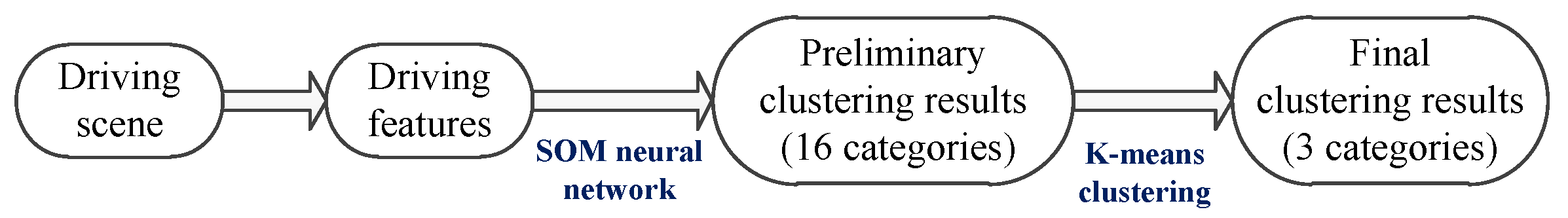
3.1. Driver Style Recognition Model

The vehicle motion and driver’s behaviors can effectively reflect the specific driving styles. Thus, a set of variables is utilized to capture the differences among various driving styles in this paper. Many previous studies utilize experimental data, including velocity, acceleration, jerk (the rate of acceleration/deceleration changes), and the opening of acceleration or braking pedal to recognize driving styles. And the statistic features of these variables, such as mean value and variance, are often taken into account. Moreover, driving styles tend to vary under different driving conditions. To robustly recognize driving styles, some feature vectors covering different driving conditions are considered in this paper, which are illustrated in

Table 1. Driving style classification features.

Driving Scenario		Feature
Low speed	Accelerating	Acceleration
		Speed
	Maintenance	Speed
		Accelerator pedal
		Jerk
Medium speed	Accelerating	Acceleration
	Maintenance	Acceleration
High speed	Accelerating	Acceleration
		Jerk
	Maintenance	Speed
		Acceleration
		Jerk
		Brake pedal

.

The vehicles selected in this paper are commercial logistics vehicles with a fixed route between Shanghai and Xuchang, China. The entire journey is 877 km, as shown in Figure 2, mainly covering highway sections, suburban sections, and some urban road conditions. In addition, 38 drivers are randomly selected to drive the experiment vehicle on the fixed route. During the driving process, an on-board telematics box (T-box) is utilized to collect vehicle data in real-time and then transmit the data to the cloud for storage. Data collected include vehicle motion states (vehicle speed, acceleration), engine states (engine speed, engine torque, and fuel consumption), and driver’s operation signals (the opening of the accelerator and brake pedal), etc. In total, 38 sets of data files are obtained and divided based on different drivers. In this way, the training data of the driving style classification model are constructed.

Based on the obtained training data, a series of data features, including mean and variance values can be calculated, which only represent a single driver sample. Furthermore, by merging all driver samples, training data have the following forms:

$$\begin{array}{c}\mathrm{X}=\{x_i\left|x_i=\left(mean\left(z_{ij}\right),\mathrm{var}iance\left(z_{ij}\right)\right)\right.;i=1,2,\dots ,N;j=1,2,3\},\end{array}$$

(1)

$$\begin{array}{c}z=\left(v,a,Jerk,p\right),\end{array}$$

(2)

where v represents velocity, a represents acceleration or deceleration, p represents the opening of the accelerator or brake pedal, N is the total number of experiment drivers, and j represents different speed intervals.

Since the style of drivers in the paper is unknown and the driver samples in the dataset are unlabeled, it is necessary to utilize unsupervised clustering methods to identify the driving style. Self-organizing map (SOM) network is an effective unsupervised clustering method, which has been proven to be highly accurate in previous clustering studies. Therefore, the SOM network is used to cluster driver samples in this paper. Typically, driver styles can be categorized into three types: conservative, moderate, and aggressive. Thus, the output of the SOM should be configured with three nodes to accommodate these distinct driving styles. However, too few output nodes can reduce the activity of the competition of the SOM. This competitive learning mechanism may reduce the accuracy of driving style recognition. Therefore, the number of output nodes of the SOM cannot be set directly to three. On the other hand, K-means is well-suited for clustering scenarios involving a limited number of categories, such as the case of recognizing driving styles. K-means functions as a clustering technique relying on Euclidean distance, where the similarity between an input vector and cluster center is quantified by the distance between the two vectors. To take advantage of the strengths of K-means and SOM, a driving style recognition method that combines K-means and SOM is illustrated in Figure 3 to solve the above issue.

In the training period, the first step is to determine the scale of the SOM network. Therefore, an empirical formula is used to determine the number of nodes in the SOM network, which can be represented as $n_{som}=5{\sqrt{N}}_{som}$, where $n_{som}$ is the number of nodes and $N_{som}$ is the sample size. Sequentially, the initial value of the weight vector $w_j$, which matches the nodes of the SOM network and its dimension is the same as the sample $x_i$, is randomly initialized. Then, all the training set samples are fed into SOM one by one, and the distance between the input vector and weight vector can be calculated by $d_j=\sqrt{{\left(x_i-w_j\right)}^T\left(x_i-w_j\right)}$. The node with the smallest $d_j$ is called as winner node, and its weight vector $w_j$ is updated by $w_j=w_j+\eta \left(x_i-w_j\right)$, where $\eta$ is the learning rate. Usually, other weight vectors also can be updated by $w_j=w_j+\eta g\left(x_i-w_j\right)$, where $g=e^{\frac{-{\left(w_i-w_j\right)}^T\left(w_i-w_j\right)}{2{\sigma }^2}}$ is called focal functions. Subsequently, the weight vector converges, and the intermediate results $z_i\in Z$ can be obtained.

The training process for K-means can be formulated as following. The only hyperparameter of K-means is the number of cluster centers. In the context of driving style recognition, the number of cluster centers is set to three. First, three samples are randomly selected as clustering centers $\{a_1,a_2,a_3\}$. Sequentially, calculate the distances of all intermediate results $z_i\in Z$ to the three cluster centers and divide them to the nearest cluster center. Subsequently, the new cluster centers can be calculated by using $a_i=\frac{1}{num}{\displaystyle \sum _{z_i\in Z}}{z}_i$, where $num$ is the sample size of category $a_i$. After reaching the maximum number of iterations, the final cluster centers of K-means can be determined.

In the context of driving style recognition, SOM is used for coarse clustering to output intermediate results, and the K-means method further clusters the intermediate results to obtain the final results of driving style recognition. After the training period, the weight vector of SOM and the cluster centers of K-means are determined. Then, the trained model can be used to recognize the driving style of each specific driver. Specifically, when the input vector $x_i$ is fed to SOM, the distance between the input vector and weight vector can be calculated, and the nearest weight vector is the intermediate result. Moreover, the intermediate result is input to a K-means model and the distance between the intermediate vector and clustering centers is calculated again. Eventually, the nearest cluster center is the final result of driving style recognition, which is shown in Figure 4.

Drivers do not have the labels in the real world, thus the recognition results of SOM+K-means cannot be verified with absolute truth. To relatively verify the recognition results of SOM+K-means, another recognition algorithm named Gaussian mixture model (GMM) is employed. The principles underlying these two recognition methods are divergent. SOM is a competitive learning algorithm where neurons compete to represent different patterns in the input data, while GMM is a generative model that models the probability distribution of the data and assigns each data point to one of the Gaussian components. If a reasonable agreement exists in the recognition results of these two algorithms, it signifies a consistent identification of the driver’s style. The recognition results of SOM+K-means and GMM algorithm are given in Figure 4. Among the 33 drivers, 23 drivers are recognized as having a conservative style by the SOM+K-means model and GMM model, 6 drivers are recognized as having a moderate style, and only 1 driver is recognized as having an aggressive style. Moreover, the recognition consistency between the SOM+K-means model and GMM model reaches 90.9%. It can be summarized that the SOM+K-means model is accurate enough to recognize the driving styles of different drivers.

3.2. Vehicle Speed Prediction Method

As illustrated in MPC-based fuel-saving control, the upcoming desired speed is used as the reference speed. A speed prediction model is designed on the basis of the learned driving style. Due to the influence of the driver’s driving style and surrounding environment, the vehicle speed has strong randomness and nonlinear properties. Considering that the inertia of commercial vehicles is higher than that of passenger vehicles, the feature of vehicle speed distribution is stable in time series. Therefore, the sequential method can be used to predict the upcoming desired speed. In this paper, a long short-term memory (LSTM) network is utilized to design the speed prediction model, and its structure is shown in Figure 5.

LSTM is a supervised learning algorithm; therefore, labeled data need to be included in the training set. In the scenario of speed prediction, the input data is the historical speed sequence of a certain period, and the output is the future speed sequence. Due to the influence of a driver’s personal driving style on the distribution of future speed, the learned driving style is also used as an input. Moreover, key vehicle states, such as acceleration, relative speed, and distance, are also considered as input variables. Finally, the training data have the following form:

$$\begin{array}{c}X=\left\{x_i\left|x_i=(f_{in,i}\left(v\right),s_1,g_{in,i}\left(s_2\right)\right.\right);i=1,2,\cdots N\},\hfill \\ Y=\{y_i\left|y_i=f_{out,i}\left(v\right)\right.;i=1,2,\cdots N\},\hfill \end{array}$$

(3)

where $f_{in}\left(v\right)$ represents the input speed series, $f_{out}\left(v\right)$ represents the output speed series, $s_1$ represents the driving style, and $s_2$ represents other key vehicle states.

While the training set $(X,Y)$ is fed to the LSTM, a forgetting gate $f\left(t\right)$ is used to forget the speed information of the previous time. Then, the current speed information $x_t$ and historical speed information $h_t$ together as input vectors enter the input gate $i\left(t\right)$, which decides what information will be retained. Finally, the output gate $o\left(t\right)$ determines the value of the speed sequence. The specific expressions for the three gating mechanisms are formulated as follows:

$$i\left(t\right)=\sigma (W_i{h}_{t-1}+W_i{x}_t+b_i),$$

(4)

$$o\left(t\right)=\sigma (W_o{h}_{t-1}+W_o{x}_t+b_o),$$

(5)

$$f\left(t\right)=\sigma (W_f{h}_{t-1}+W_f{x}_t+b_f),$$

(6)

where $W_i$, $W_o$, and $W_f$ are the weights in the input gate, output gate, and forgetting gate, respectively, $\sigma$ represents the activation function, and $b_i$, $b_o$, and $b_f$ represent the bias in the input gate, output gate, and forgetting gate, respectively.

After the parameters of the LSTM are determined, the process of speed prediction can be formulated as follows. Firstly, feature data $x_t$, including historical speed series, the learned driving style, and key vehicle states, are fed to the LSTM. Using the forgetting gate $f_t$ and the input gate $i_t$, intermediate variables $c_t$ can be obtained. Then, $c_t$ is used to output the future speed series from gate $o_t$. The aforementioned process can be represented as:

$${\tilde{c}}_t=tanh(W_c{h}_{t-1}+W_c{x}_t+b_c),$$

(7)

$$c_t=f_t\odot c_{t-1}+i_t\odot {\tilde{c}}_t,$$

(8)

$$h_t=o_t\odot tanh\left(c_t\right),$$

(9)

where the activation function tanh$\left(x\right)=\frac{e^x-e^{-x}}{e^x+e^{-x}}$, $x_t$ represents the input vector, $c_t$ represents the state of LSTM cell at time t, $h_t$ represents the output of LSTM, and ⊙ represents the multiplication between each element. In the period of validation, the upcoming desired speed is predicted by $h_t$.

4. Design of the MPC-Based Optimal Controller

This section aims to design an MPC-based optimal controller to enhance fuel efficiency in human–machine collaborative driving. The subsequent subsections present a detailed overview of key design steps. Firstly, the construction of the system model for the commercial vehicle is outlined, as the design of the MPC-based optimal controller relies on a model-based approach. Next, the formulation of the optimization problem is discussed, wherein the driver’s intentions are integrated with the fuel-saving objectives to achieve collaborative driving control. Subsequently, predictive equations are provided, as MPC, also known as receding horizon control, utilizes predictions of system’s future states. Finally, the solution is derived to effectively address the optimization problem.

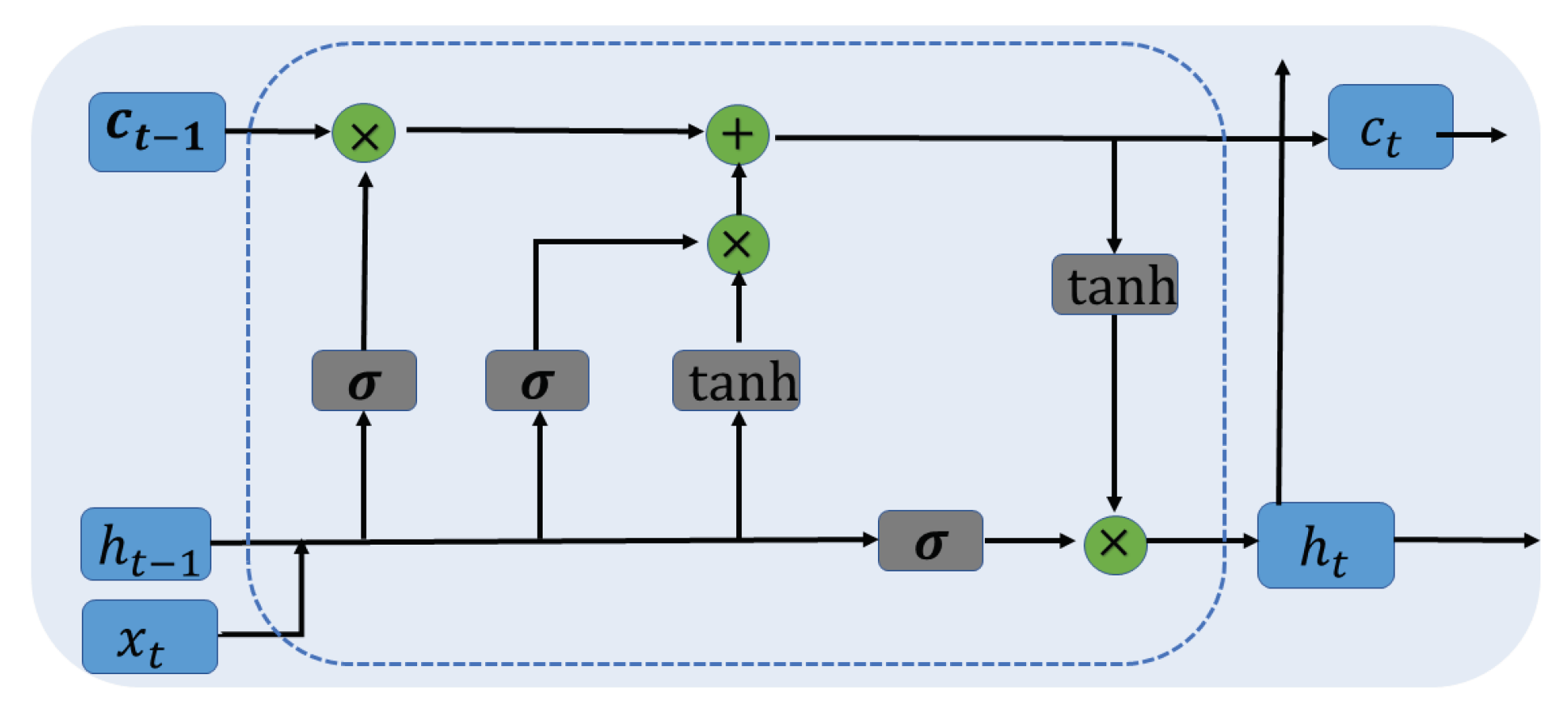
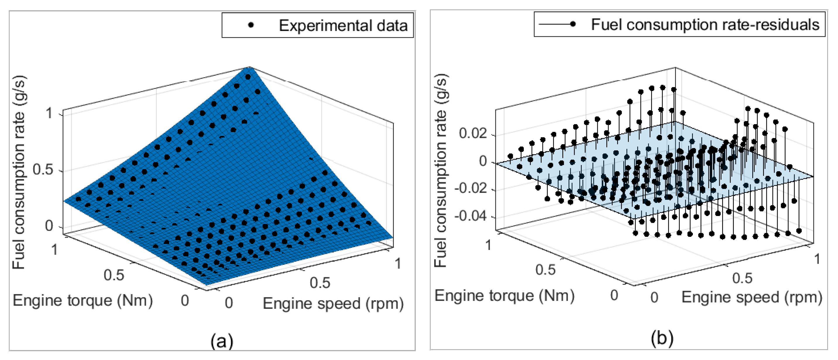
4.1. System Modeling of Commercial Vehicles

The vehicle under discussion is a heavy-duty commercial vehicle. When the vehicle is driving on the road, the longitudinal motion model can be described as follows:

$$\begin{array}{cc}\hfill \dot{s}& =v\hfill \\ \hfill \dot{v}& =a,\hfill \end{array}$$

(10)

where s is the driving distance of the vehicle, v is the vehicle speed, and a is the vehicle acceleration. The longitudinal acceleration a is determined by the force balance equation

$$F_t=F_w+F_f+F_i+F_j,$$

(11)

where $F_t$, $F_w$, $F_f$, $F_i$, $F_j$ are the traction force, air resistance, rolling resistance, slope resistance, and acceleration resistance. Further expanding each item of Equation (11), the longitudinal dynamics of the commercial vehicle in the traction model can be summarized as follows:

$$\frac{\eta I_f{I}_g}{r}{T}_e=\frac{1}{2}{C}_d{A}_f\rho v^2+\mu Mgcos\left(\alpha \right)+Mgsin\left(\alpha \right)+\delta Ma,$$

(12)

where $\eta$ is the mechanical efficiency of the transmission system, M is the vehicle mass, $T_e$ is the engine torque, $I_f$ is the transmission ratio of the vehicle’s main reducer, $I_g$ is the transmission ratio of the vehicle’s gearbox, and r is the wheel radius, $\mu$ is the friction coefficient of the vehicle on the road, $\alpha$ is the road slope, g is the acceleration of gravity, $C_d$ is the air resistance coefficient in the driving environment of the vehicle, and $A_f$ is the frontal area of the vehicle, $\rho$ is the density of air, and $\delta$ is the lumped rotational inertia coefficient.

When the commercial vehicle is working in the brake mode, the engine provides a drag resistance force $T_{e,drag}$. The longitudinal dynamics become

$$\frac{I_f{I}_g}{\eta r}{T}_{e,drag}=\frac{1}{2}{C}_d{A}_f\rho v^2+\mu Mgcos\left(\alpha \right)+Mgsin\left(\alpha \right)+\delta Ma.$$

(13)

To facilitate the design of the fuel-saving controller, it is necessary to obtain an accurate fuel consumption model. Typically, the fuel consumption model is expressed in polynomial form. The parameters of the polynomial are acquired using the method of least squares. In line with the approach outlined in [10], the polynomial model employed for the engine fuel consumption used in this study is as follows:

$${\dot{m}}_f(n_e,T_e)=\sum _{i=0}^2\sum _{j=0}^2{\iota }_{i,j}{T_e}^i{n}_e^j,$$

(14)

where $n_e$ is the engine speed, and ${\iota }_{i,j}$ represents the fitting coefficients.

The fitting coefficients are obtained using the method of least squares. Figure 6 depicts the fitting performance of the engine fuel consumption model. Black dots are the experimental data points. The experimental data in Figure 6 are the normalized data. It can be seen from Figure 6 that the experimental data points are evenly distributed near the fitted surface, which means the fitted polynomial model has a good approximation performance. The root mean square error between the experimental data and the fitted model is 0.01871.

Using the conversion relationship between vehicle speed v and engine speed $n_e$

$$v=2\pi r_w\frac{n_e}{60\times I_f{I}_g},$$

(15)

the following fuel consumption model can be obtained as follows:

$${\dot{m}}_f(v,T_e)=p_1{v}^2+p_2{T}_e^2+p_{3}v{T}_e+p_{4}v+p_5{T}_e,$$

(16)

where $p_i$ are the converted coefficients from the fitting coefficients ${\iota }_{i,j}$.

4.2. Formulation of Multi-Objective Function

The objective of the fuel-saving-oriented collaborative driving system is to fulfill the driver’s intentions while minimizing fuel consumption to the greatest extent possible. To accomplish this objective, three key goals are devised: (1) minimizing the tracking error of the driver’s desired speed, (2) minimizing fuel consumption, and (3) minimizing engine torque ripple.

4.2.1. Minimizing the Tracking Error of the Driver’s Desired Speed

The driver’s desired speed represents their intended longitudinal behavior for the vehicle, taking into account subjective power demand and driving safety considerations. A deficiency in tracking the driver’s desired speed can yield unfavorable outcomes, such as the driver frequently needing to readjust the opening of the accelerator pedal, which subsequently results in increased fuel consumption. Thus, the problem of satisfying the driver’s intent is transformed into a speed tracking problem. To guarantee alignment with the driver’s intention, the first cost function is defined as follows:

$$J_v=\sum _{k=1}^N{w}_r{(v\left(k\right)-v_r\left(k\right))}^2\Delta t,$$

(17)

where N is the length of the prediction horizon, $w_r$ is the weight coefficient of the speed tracking term, $v\left(k\right)$ is the vehicle speed at step k, and $v_r\left(k\right)$ is the desired speed of the driver at step k.

4.2.2. Minimizing Fuel Consumption

The primary objective of the proposed collaborative driving system is to enhance fuel-saving performance. To quantify the fuel consumption, the system utilizes the fitting polynomial of the fuel consumption and defines the fuel consumption index as follows:

$$J_Q=\sum _{k=1}^N{w}_f{\dot{m}}_f(v\left(k\right),T_e\left(k\right))\Delta t,$$

(18)

where $w_f$ is the weight coefficient of the fuel consumption item.

4.2.3. Minimizing Engine Torque Ripple

To reduce the ripple of the engine torque and ensure a smooth change in engine torque, a cost function for minimizing engine torque ripple is designed as follows:

$$J_u=\sum _{k=1}^N{w}_u{u}^2\left(k\right)\Delta t,$$

(19)

where $w_u$ is the weight coefficient of the engine torque ripple item, and $u_k$ is the control input, namely the change rate of the engine torque.

On the basis of the above cost functions, the multi-objective function is formulated as follows:

$$\begin{array}{cc}\hfill J=& J_v+J_Q+J_u\hfill \\ \hfill =& \sum _{k=1}^N[w_r{(v\left(k\right)-v_r\left(k\right))}^2+w_f{\dot{m}}_f(v\left(k\right),T_e\left(k\right))+w_u{u}^2\left(k\right)]\Delta t\hfill \end{array}$$

(20)

The multi-objective function shows that these three penalty terms are in conflict with each other. Achieving a perfect tracking of the desired speed is often at the expense of engine torque fluctuation, which results in increased fuel consumption. Consequently, the selection of appropriate weighting coefficients requires a trade-off between these conflicting objectives.

By the substitution of Equation (16) into Equation (20), the multi-objective function becomes

$$\begin{array}{cc}\hfill J=& \sum _{k=1}^N[((p_1+w_r)v^2\left(k\right)+p_2{T}_e^2\left(k\right)+p_{3}v\left(k\right)T_e\left(k\right))\Delta t\hfill \\ \hfill & +((p_4-2w_r{v}_r\left(k\right))v\left(k\right)+p_5{T}_e\left(k\right))\Delta t+w_u{u}^2\left(k\right)\Delta t]\hfill \\ \hfill =& \sum _{k=1}^N[{\tilde{x}}^T\left(k\right)Q\tilde{x}\left(k\right)+C\tilde{x}\left(k\right)+u^T\left(k\right)\mathrm{R}u\left(k\right)]\hfill \end{array}$$

(21)

where $\tilde{x}\left(k\right)=\left[\begin{array}{c}v\left(k\right)\\ T_e\left(k\right)\end{array}\right]$, $Q=\left[\begin{array}{cc}(p_1+w_r)\Delta t& \frac{p_3\Delta t}{2}\\ \frac{p_3\Delta t}{2}& p_2\Delta t\end{array}\right]$, $C={\left[\begin{array}{c}(p_4-2w_r{v}_r\left(k\right))\Delta t\\ p_5\Delta t\end{array}\right]}^T$, $R=w_u\Delta t$.

The presence of a first-order item, $C\tilde{x}\left(k\right)$, is evident in the multi-objective function (21). To handle this, two additional variables, ${\Delta }_1\left(k\right)$ and ${\Delta }_2\left(k\right)$, are introduced, and a new state matrix is defined as $x\left(k\right)=\left[\begin{array}{c}v\left(k\right)+{\Delta }_1\left(k\right)\\ T_e\left(k\right)+{\Delta }_2\left(k\right)\end{array}\right]=\tilde{x}\left(k\right)+\Delta \left(k\right)$. By utilizing this newly defined state matrix, the multi-objective function (21) can be transformed as follows:

$$\begin{array}{cc}\hfill J=& \sum _{k=1}^N\left[{\left(x\left(k\right)-\Delta \left(k\right)\right)}^{T}Q\left(x\left(k\right)-\Delta \left(k\right)\right)+C\left(x\left(k\right)-\Delta \left(k\right)\right)+u^T\left(k\right)Ru\left(k\right)\right]\hfill \\ \hfill =& \sum _{k=1}^N\left[x^T\left(k\right)Qx\left(k\right)+u^T\left(k\right)Ru\left(k\right)+\left(C-2{\Delta }^T\left(k\right)Q\right)x\left(k\right)+{\Delta }^T\left(k\right)Q\Delta \left(k\right)-C\Delta \left(k\right)\right].\hfill \end{array}$$

(22)

If $\Delta \left(k\right)={\left(\frac{1}{2}C{Q}^{-1}\right)}^T$, then $J={\displaystyle \sum _{k=1}^N}{x}^T\left(k\right)Qx\left(k\right)+u^T\left(k\right)Ru\left(k\right)+{\Delta }^T\left(k\right)Q\Delta \left(k\right)-C\Delta \left(k\right)$. In this transformation of the multi-objective function, item ${\Delta }^T\left(k\right)Q\Delta \left(k\right)-C\Delta \left(k\right)$ is omitted since it is not related to the variable to be optimized. The multi-objective function (22) becomes

$$\begin{array}{c}\hfill J=\sum _{k=1}^N{x}^T\left(k\right)Qx\left(k\right)+u^T\left(k\right)Ru\left(k\right).\end{array}$$

(23)

Evidently, the cost function (23) is quadratic, which makes it easier to find a solution of the optimization problem.

4.3. Predictive Equation

Predictive equations play a crucial role in MPC because they enable the controller to make decisions based on predictions of the system’s future states and outputs. By utilizing predictive equations, the MPC controller can optimize its control actions over a future time horizon to achieve desired performance objectives.

Taking vehicle speed and engine torque as vehicle states, the mathematical model for the time-domain discretization is presented as follows:

$$\left\{\begin{array}{c}v(k+1)=v\left(k\right)+\mathrm{a}\left(k\right)T_{\mathrm{s}}\hfill \\ T_e(k+1)=T_e\left(k\right)+{\dot{T}}_e\left(k\right)T_{\mathrm{s}},\hfill \end{array}\right.,$$

(24)

where $T_{\mathrm{s}}$ is the sample time interval and ${\dot{T}}_e$ is the change rate of the engine torque. By substituting Equation (12) into Equation (24), the longitudinal dynamic model used for prediction equations is obtained

$$\left\{\begin{array}{c}v(k+1)=v\left(k\right)+T_{\mathrm{s}}(\frac{\eta I_f{I}_g{T}_e\left(k\right)}{\delta Mr}-\frac{\mu gcos\left(\alpha \right)}{\delta }-\frac{gsin\left(\alpha \right)}{\delta }-\frac{C_d{A}_f\rho }{2\delta M}{v}^2\left(k\right))\hfill \\ T_e(k+1)=T_e\left(k\right)+T_{\mathrm{s}}{\dot{T}}_e\left(k\right)\hfill \end{array}\right.,$$

(25)

In the construction of a quadratic objective function, two additional variables of ${\Delta }_1\left(k\right)$ and ${\Delta }_2\left(k\right)$ are used. For consistency, the state equation of the discrete system is given as follows:

$$\left\{\begin{array}{c}x(k+1)=Ax\left(k\right)+B_{u}u\left(k\right)+B_{d}d\left(k\right)\hfill \\ y\left(k\right)=C_{c}x\left(k\right)\hfill \end{array}\right.,$$

(26)

where $x\left(k\right)=\left[\begin{array}{c}v\left(k\right)+{\Delta }_1\left(k\right)\\ T_e\left(k\right)+{\Delta }_2\left(k\right)\end{array}\right]$, $u\left(k\right)={\dot{T}}_e\left(k\right)$, $A=\left[\begin{array}{cc}1& \frac{T_s\eta I_f{I}_g}{M{r}_w\delta }\\ 0& 1\end{array}\right]$, $B_u=\left[\begin{array}{c}0\\ T_s\end{array}\right]$, $d\left(k\right)=\left[\begin{array}{c}{T}_s\left(\frac{-\eta I_f{I}_g{\Delta }_2\left(k\right)}{M\delta r_{\mathrm{w}}}-\frac{\mu gcos\left(\alpha \right)}{\delta }-\frac{gsin\left(\alpha \right)}{\delta }-\frac{C_d{A}_f\rho }{2M\delta }{v}^2\left(k\right)\right)+{\Delta }_1(k+1)-{\Delta }_1\left(k\right)\\ {\Delta }_2(k+1)-{\Delta }_2\left(k\right)\end{array}\right]$, $B_u=\left[\begin{array}{c}0\\ T_s\end{array}\right]$, $B_d=C_c=I_{2\times 2}$, and I is the identity matrix.

Beginning from the initial step k, through repeated substitution, the states of the discrete system at step $k+i$ can be obtained as

$$\begin{array}{c}x(k+i\left|k\right.)=A^{i}x\left(k\right)+{\displaystyle \sum _{j=1}^i}\left[A^{j-1}{B}_{u}u(k+i-j)+A^{j-1}{B}_{d}d(k+i-j)\right],\hfill \end{array}$$

(27)

The outputs of the discrete system at step $k+i$ is

$$\begin{array}{c}y(k+i\left|k\right.)={\displaystyle \sum _{j=1}^i}\left[C_c{A}^{j-1}{B}_{u}u(k+i-j)+C_c{A}^{j-1}{B}_{d}d(k+i-j)\right]\hfill \\ +{\displaystyle \sum _{j=1}^i}{C}_c{A}^{i}x\left(k\right),\hfill \end{array}$$

(28)

Defining the predicted output as $Y_p(k+1\left|k)\right.\stackrel{\Delta }{=}{\left[\begin{array}{c}y(k+1\left|k)\right.\\ y(k+2\left|k)\right.\\ ⋮\\ y(k+p\left|k)\right.\end{array}\right]}_{p\times 1}$, the future control input as $U\left(k\right)\stackrel{\Delta }{=}{\left[\begin{array}{c}u\left(k\right)\\ u(k+1)\\ ⋮\\ u(k+p-1)\end{array}\right]}_{p\times 1}$, and the external disturbance item as $D\left(k\right)\stackrel{\Delta }{=}{\left[\begin{array}{c}d\left(k\right)\\ d(k+1)\\ ⋮\\ d(k+p-1)\end{array}\right]}_{p\times 1}$ and using Equations (27) and (28), the predictive system model (26) can be transformed into the following form:

$$\begin{array}{c}{Y}_p(k+1\left|k\right.)={\mathcal{S}}_{x}x\left(k\right)+{\mathcal{S}}_{u}U\left(k\right)+{\mathcal{S}}_{d}D\left(k\right),\hfill \end{array}$$

(29)

where p is the prediction and control horizon. The coefficients in the prediction Equation (29) are ${\mathcal{S}}_x={\left[\begin{array}{c}{C}_{c}A\\ C_c{A}^2\\ ⋮\\ C_c{A}^p\end{array}\right]}_{p\times 1}$, ${\mathcal{S}}_u={\left[\begin{array}{cccc}{C}_c{B}_u,& 0,& \cdots ,& 0\\ C_{c}A{B}_u,& C_c{B}_u,& \cdots ,& 0\\ C_c{A}^2{B}_u,& C_{c}A{B}_u,& \cdots ,& 0\\ ⋮& ⋮& \ddots & ⋮\\ C_c{A}^{p-1}{B}_u,& C_c{A}^{p-2}{B}_u,& \cdots ,& C_c{B}_u\end{array}\right]}_{p\times p}$, and ${\mathcal{S}}_d={\left[\begin{array}{cccc}{C}_c{B}_d,& 0,& \cdots ,& 0\\ C_{c}A{B}_d,& C_c{B}_d,& \cdots ,& 0\\ C_c{A}^2{B}_d,& C_{c}A{B}_d,& \cdots ,& 0\\ ⋮& ⋮& \ddots & ⋮\\ C_c{A}^{p-1}{B}_d,& C_c{A}^{p-2}{B}_d,& \cdots ,& C_c{B}_d\end{array}\right]}_{p\times p}$.

4.4. Solution of the Optimization Problem

Using the predictive system model (29), the multi-objective function (22) can be transformed as follows:

$$\begin{array}{cc}\hfill J\left(x\left(k\right),U\left(k\right),n\right)& =\sum _{k=1}^N[x^T\left(k\right)Qx\left(k\right)+u^T\left(k\right)Ru\left(k\right)]\hfill \\ \hfill & ={\left({\Gamma }_y{Y}_p(k+1|k)\right)}^T\left({\Gamma }_y{Y}_p(k+1|k)\right)+{∥{\Gamma }_{u}U\left(k\right)∥}^2\hfill \\ \hfill & ={\left[\begin{array}{c}{\Gamma }_y{Y}_p(k+1\mid k)\\ {\Gamma }_{u}U\left(k\right)\end{array}\right]}^T\left[\begin{array}{c}{\Gamma }_y{Y}_p(k+1\mid k)\\ {\Gamma }_{u}U\left(k\right)\end{array}\right],\hfill \end{array}$$

(30)

where the weight matrix ${\Gamma }_y=diag({\Gamma }_{y,1},{\Gamma }_{y,2},\dots ,{\Gamma }_{y,p})$ with ${\Gamma }_{y,i}^{{}^T}{\Gamma }_{y,i}=Q$, and the weight matrix ${\Gamma }_u=diag({\Gamma }_{u,1},{\Gamma }_{u,2}\dots {\Gamma }_{u,p})$ with ${\Gamma }_{u,j}^{{}^2}=R$. Clearly, the weight matrices $\Gamma y$ and $\Gamma u$ are determined by the weight coefficient of the objective term and remain constant throughout the predictive horizon.

To facilitate the solution of the optimization problem, an auxiliary variable is defined as

$$\begin{array}{cc}\hfill \rho \stackrel{\Delta }{=}\left[\begin{array}{c}{\Gamma }_y{Y}_p(k+1\left|k)\right.\\ {\Gamma }_{u}U\left(k\right)\end{array}\right]& =\left[\begin{array}{c}{\Gamma }_y{\mathcal{S}}_u\\ {\Gamma }_u\end{array}\right]U\left(k\right)+\left[\begin{array}{c}{\Gamma }_y{\mathcal{S}}_{x}x\left(k\right)+{\Gamma }_y{\mathcal{S}}_{d}D\left(k\right)\\ 0\end{array}\right]\hfill \\ \hfill & =A_{z}z+b\hfill \end{array}$$

(31)

where $A_z=\left[\begin{array}{c}{\Gamma }_y{\mathcal{S}}_u\\ {\Gamma }_u\end{array}\right]$, $z=U\left(k\right)$ and $b=\left[\begin{array}{c}{\Gamma }_y{\mathcal{S}}_{x}x\left(k\right)+{\Gamma }_y{\mathcal{S}}_{d}D\left(k\right)\\ 0\end{array}\right]$. The multi-objective optimization problem can be written as

$$\underset{z}{min}J=\underset{z}{min}{\rho }^T\rho .$$

(32)

The optimal solution can be found as

$$\left\{\begin{array}{c}\frac{d\left({\rho }^T\rho \right)}{dz}=2A_z^T\left(A_{z}z+b\right)=0\\ \frac{d^2\left({\rho }^T\rho \right)}{d{z}^2}=2A_z^T{A}_z>0\end{array}\right.⟹z={\left(A_z^T{A}_z\right)}^{-1}(-A_{z}b).$$

(33)

Then, the solution of the optimization problem is

$$U\left(k\right)=-{\left({\mathcal{S}}_u^T{\Gamma }_y^T{\Gamma }_y{\mathcal{S}}_u+{\Gamma }_u^T{\Gamma }_u\right)}^{-1}\left[{\mathcal{S}}_u^T{\Gamma }_y^T{\Gamma }_y\left({\mathcal{S}}_{x}x\left(k\right)+{\mathcal{S}}_{d}D\left(k\right)\right)\right]$$

(34)

The current control input is determined solely by the first element of each solution sequence. The iterative process will persist at each subsequent horizon.

5. Human–Machine Collaboration

The human–machine collaboration is introduced to provide a trade-off input by blending driver input and controller input. The trade-off lies in ensuring both meeting the driver’s intentions and achieving good fuel efficiency. When the controller is inactive, the driver’s pedal operation directly serves as the engine’s torque demand. The driver’s operation to the vehicle’s response is straightforward. However, when the controller is activated, the driver’s control of the vehicle becomes less direct. Considering the driver’s sensitivity to real-time power feedback from the vehicle, it is typically desired to minimize the discrepancy between the actual engine torque applied to the vehicle and the driver’s desired torque.

A simple collaborative rule is proposed to ensure alignment with the driver’s intention. This collaborative rule is implemented by introducing upper and lower thresholds to control the direction of the deviation. When there is an upward deviation between the controller’s input and the driver’s input, the upper threshold comes into play to adjust the controller’s output towards the driver’s input. Similarly, when there is a downward deviation, the lower threshold comes into play to align the controller’s output with the driver’s input. Through this straightforward collaborative rule, consistency between the driver and the controller is maintained, thereby better achieving the objectives of human–machine collaborative driving.

By introducing the lower and upper thresholds ${\alpha }_1$ and ${\alpha }_2$, the system input is governed by a collaborative rule as expressed by the following equation:

$$T_e^{ref}=\left\{\begin{array}{cc}\left(1-{\alpha }_1\right)T_{e,d},& T_{e,c}<\left(1-{\alpha }_1\right)T_{e,d}\\ T_{e,c},& \left(1-{\alpha }_1\right)T_{e,d}<T_{e,c}<\left(1+{\alpha }_2\right)T_{e,d}\\ \left(1+{\alpha }_2\right)T_{e,d},& \left(1+{\alpha }_2\right)T_{e,d}<T_{e,c}\end{array}\right.$$

(35)

where $T_{e,d}$ is the driver’s desired engine torque, and $T_{e,c}$ is the control input of the optimal controller. The driver’s desired engine torque, which depends on the position of the accelerator pedal, can be acquired using a two-dimensional pedal map. The control input of the optimal controller is derived from the first element of each solution sequence. Finally, $T_e^{ref}$ is applied to the engine system to determine the vehicle’s state at the next moment.

6. Results and Discussion

To evaluate the fuel-saving performance of the proposed human–machine co-driving system, both simulations and experiments are carried out. The accuracy and effectiveness of the vehicle speed prediction are verified using real-world driving data. Following this, a detailed evaluation is performed to validate the fuel-saving performance under medium-speed and high-speed driving conditions.

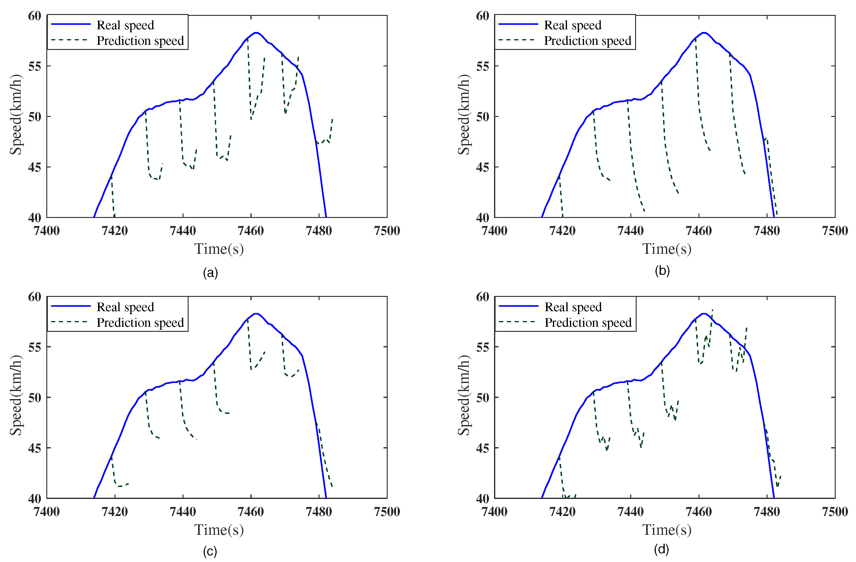
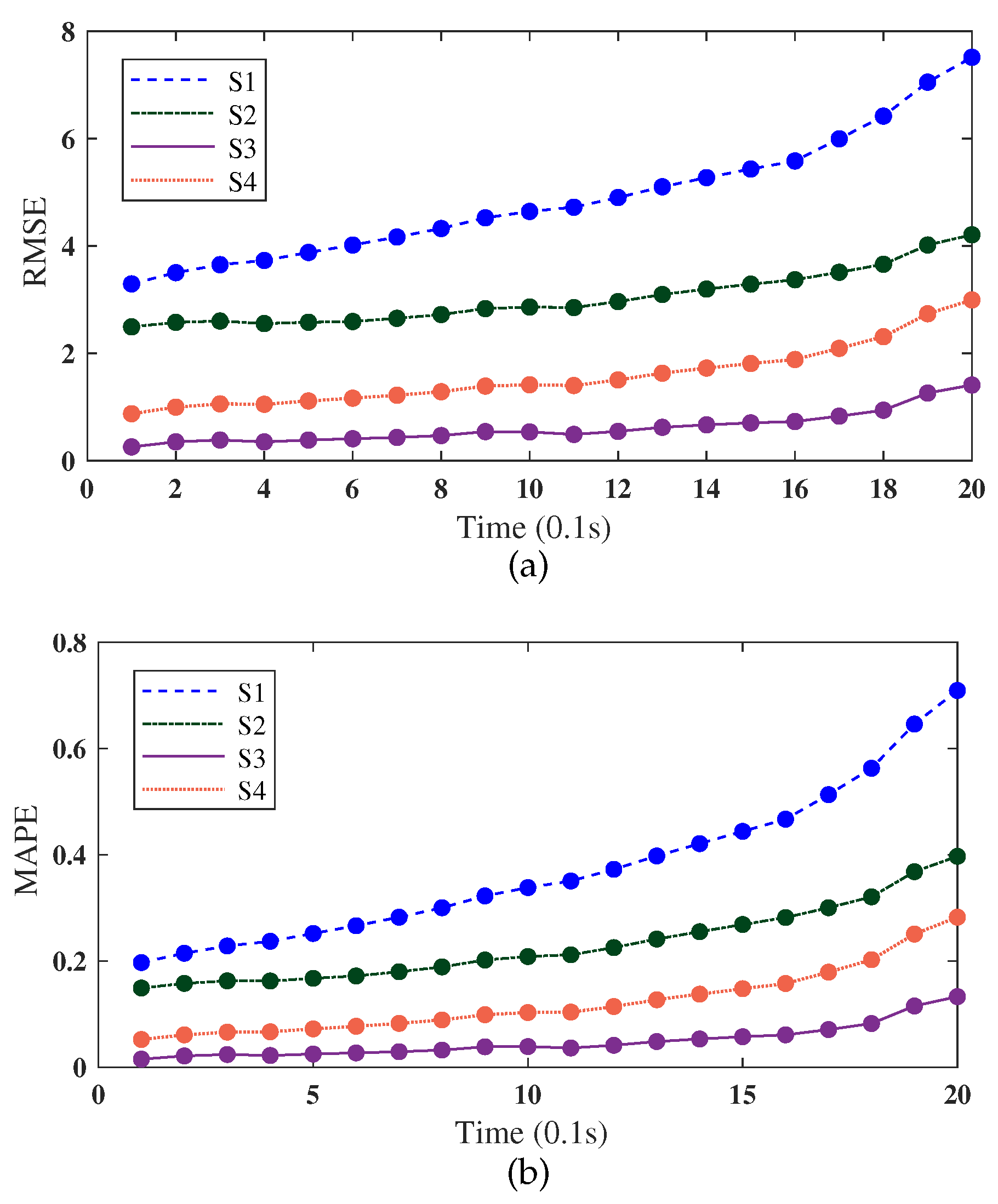
6.1. Vehicle Speed Prediction

To thoroughly evaluate the effectiveness of the velocity prediction method, a set of comparative experiments is carried out, incorporating a range of signal inputs. Additionally, a comprehensive investigation is conducted to analyze the impact of driving style on the ability to predict speed. The present analysis encompasses the execution of prediction experiments, wherein driver style labels are included in some instances and excluded in others. Subsequently, the prediction error is carefully analyzed and discussed.

The test data used in this study comprises approximately 10 h of real driving data. The dataset is divided into two subsets: the training set, which constitutes the initial 70% of the data, and the testing set, comprising the remaining 30%. This division allows for comprehensive model training and subsequent testing to assess the prediction performance.

6.1.1. Input Feature Selection

The selection of input features directly affects the performance of the prediction. The key features consist of the historical vehicle speed, the historical acceleration, the driver’s driving style, and the relative distance and speed between the host vehicle and the preceding vehicle. Taking into account computational resources and model complexity, a three-feature input is selected, incorporating features of historical speed (Spe), driving style (Dri-Sty), and an additional key feature such as acceleration (Acc), relative speed (Rela-Spe), and relative distance (Rela-Dis). The design of the three-feature input is presented in

Table 2. Settings of input features. (* indicates that the feature is selected).

Variable	Spe	Dri-Sty	Acc	Rela-Spe	Rela-Dis
S1	*	*
S2	*	*	*
S3	*	*		*
S4	*	*			*

.

In vehicle speed prediction, the historical data consists of 100 steps, and the prediction horizon spans 20 steps, with each step having a time interval of 0.1 s. The obtained prediction results are illustrated in Figure 7. The partial enlarged view of Figure 7 is shown in Figure 8. The analysis reveals that speed prediction stability under setting S1 is relatively poor, and the accuracy of speed prediction diminishes significantly after a certain number of prediction steps. Notably, for scenarios involving changes in speed increments or decrements, the prediction performances of settings S3 and S4 outperform that of setting S2. Specifically, the prediction accuracy and stability of S3 are superior to those of S4.

The speed prediction results were further analyzed using quantitative methods, wherein the evaluation metrics of root mean square error (RMSE) and mean absolute percentage error (MAPE) were selected. The variations of RMSE and MAPE for the four different settings are depicted in Figure 9. It is evident that prediction errors increase as the prediction steps increase. Among the evaluated settings, the output results of S3 demonstrated superior accuracy and stability compared to the others. Consequently, for the subsequent implementation, S3 was selected as the feature input.

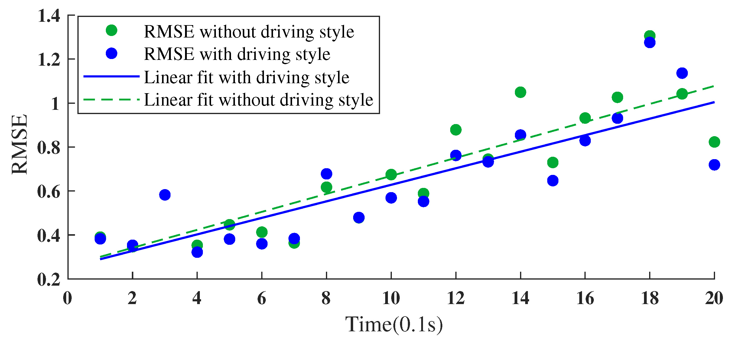
6.1.2. Effect of Driving Style on Velocity Prediction

The influence of driving style on speed prediction was further evaluated in two scenarios: with and without driving style input. The same model parameters were utilized, following the input set presented in

Table 3. Settings of input features. (* indicates that the feature is selected).

Variable	Spe	Rela-Spe	Dri-Sty
S3	*	*	*
S5	*	*

. The speed prediction results were recorded, and the corresponding error values were obtained. All the prediction errors in each prediction step are summed and averaged. The results are shown in Figure 10, with each data point representing the averaged value at the respective prediction step. To highlight the performance improvement achieved by introducing the driving style feature, the errors (RMSE) for different inputs were fitted using the least squares method. The fitted functions for cases without and with the introduction of driving styles are expressed as follows:

• Without driving style feature: $RMSE\left(t\right)=0.0409t+0.2597$
• With driving style feature: $RMSE\left(t\right)=0.0376t+0.2521$

It can be seen from Figure 10 that the inclusion of the driving style feature in the input enhances the overall prediction accuracy compared to the scenario without the introduction of the driving style input.

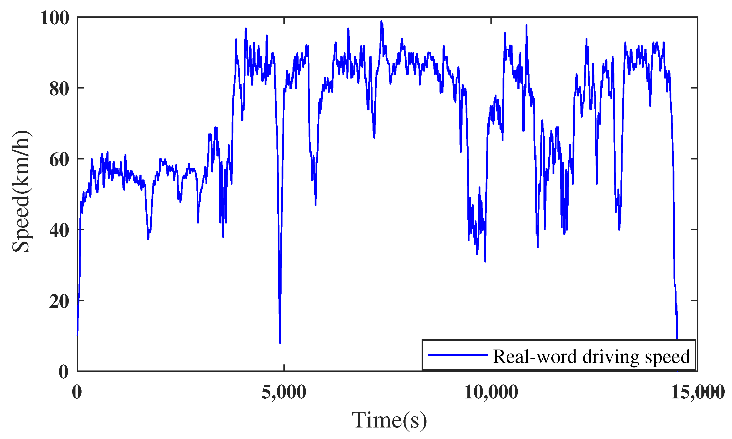
6.2. Evaluation on Fuel-Saving Performance

Simulations are conducted to assess the fuel-saving performance of the proposed human–machine co-driving system, utilizing real-world driving data as the speed reference. The human–machine co-driving system is implemented within the Simulink/Matlab environment. To ensure comparability, the drivers and driving tasks remain consistent both before and after incorporating the proposed system. For simulating the behavior of human drivers, a speed-tracing PID controller is employed. During the simulations, the control horizon and prediction horizon are both set to twenty, and the total prediction domain spans 2 s. To establish a suitable range of speeds for validation, we utilize data on the typical speeds at which the vehicle operates during daily driving. Subsequently, the fuel consumption performance is verified within this speed range.

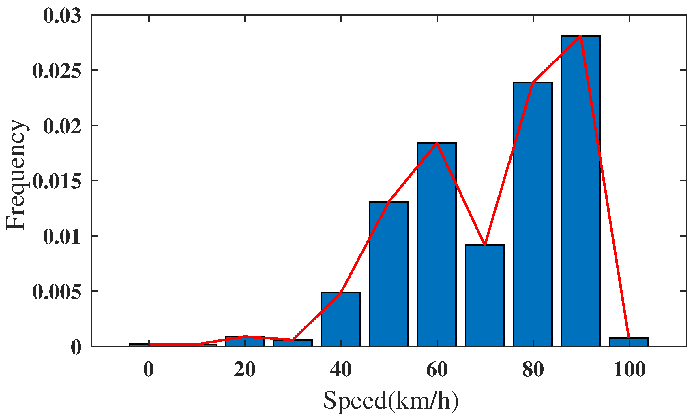
6.2.1. Speed Range Selection

The commercial vehicles under investigation predominantly operate on a specific route, and the speed profile of real vehicle data is depicted in Figure 11. Probability distribution graphs are presented in Figure 12 with a speed range of 10 km/h used for the proportion statistics to evaluate the distributions of the speed profile quantitatively. Based on the distribution of vehicle speeds, three distinct speed ranges are defined: the low-speed range (0 km/h–30 km/h), the medium-speed range (30 km/h–60 km/h), and the high-speed range (above 60 km/h).

From Figure 12, it is evident that there are fewer recorded data points when the vehicle speed falls within the low-speed range (0 km/h–30 km/h). This observation suggests that the vehicle spends relatively less time driving within this speed range, and the fuel consumption in this range has a minor impact on the entire driving cycle. Therefore, high-speed range and medium-speed range are selected for assessing fuel-saving performance.

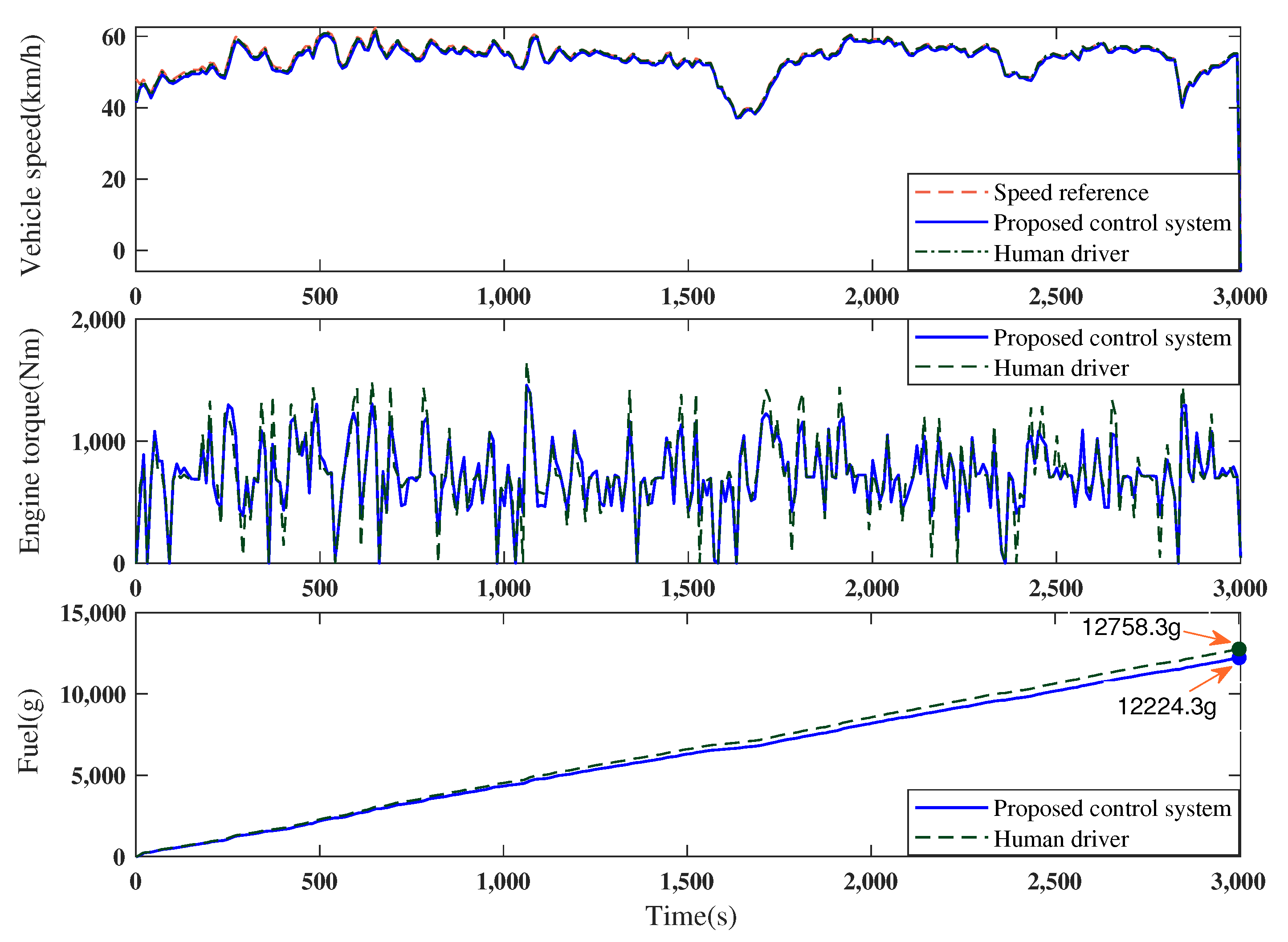
6.2.2. Comparison of Performance in the High-Speed Range

Performance in the high-speed range is first evaluated. Simulation results are shown in Figure 13. It can be seen from Figure 13 that, in comparison to the driver without the human–machine collaboration, the driver utilizing the human–machine collaboration achieves not only reliable speed tracking performance but also a certain smoothing effect on the vehicle speed, effectively suppressing local speed fluctuations. Furthermore, the sudden torque changes of the engine are suppressed for drivers with the human–machine collaboration, resulting in smoother engine torque variations and reduced peak torque. These efforts to suppress speed and engine torque fluctuations contribute not only to improved driving comfort but also to an enhancement of the vehicle’s overall fuel economy.

The utilization of human–machine collaboration leads to adjustments in engine torque and vehicle speed profile, ultimately improving the vehicle’s fuel economy and reducing the overall fuel consumption. The proposed human–machine co-driving system achieves a fuel saving rate of 3.04% without compromising the speed tracking performance.

6.2.3. Comparison of Performance in the Medium-Speed Range Range

Performance in the medium-speed range is evaluated, and simulation results are presented in Figure 14. As depicted in Figure 14, the performance of the proposed human–machine co-driving system in the medium-speed range is comparable to that observed in the high-speed range. Concerning vehicle speed, the proposed system exhibits the capability to maintain smooth vehicle speed while effectively tracking the driver’s desired speed. Regarding the engine torque, the system achieves smoother torque variations and suppresses sudden changes. The proposed human–machine co-driving system yields a fuel-saving rate of 4.1% without compromising speed tracking performance.

Table 4. Comparison of fuel-saving performance.

Method Conditions	High-Speed Range	Medium-Speed Range
Driver	27,754.6 g	12,758.3 g
Proposed control system	26,897.4 g	12,224.3 g
Fuel saving rate	3.04%	4.1%

summarizes the performance comparison in both the high-speed range and medium-speed range. The comparison reveals that the proposed human–machine co-driving system achieves a fuel saving rate of 3–4% more than that of human drivers, in both the medium and high-speed ranges.

7. Conclusions

Driver-centered energy-saving techniques have enormous potential for commercial vehicles. The paper proposes an innovative collaborative driving strategy aimed at fuel conservation in the context of commercial vehicles. The collaborative driving strategy encompasses a sequence of crucial components: driving style recognition, the prediction of desired vehicle speed, the formulation of an MPC-based optimal controller, and the establishment of a collaborative rule. Finally, the proposed control scheme is validated through simulation and real-world driving data. The validation process unfolds as follows:

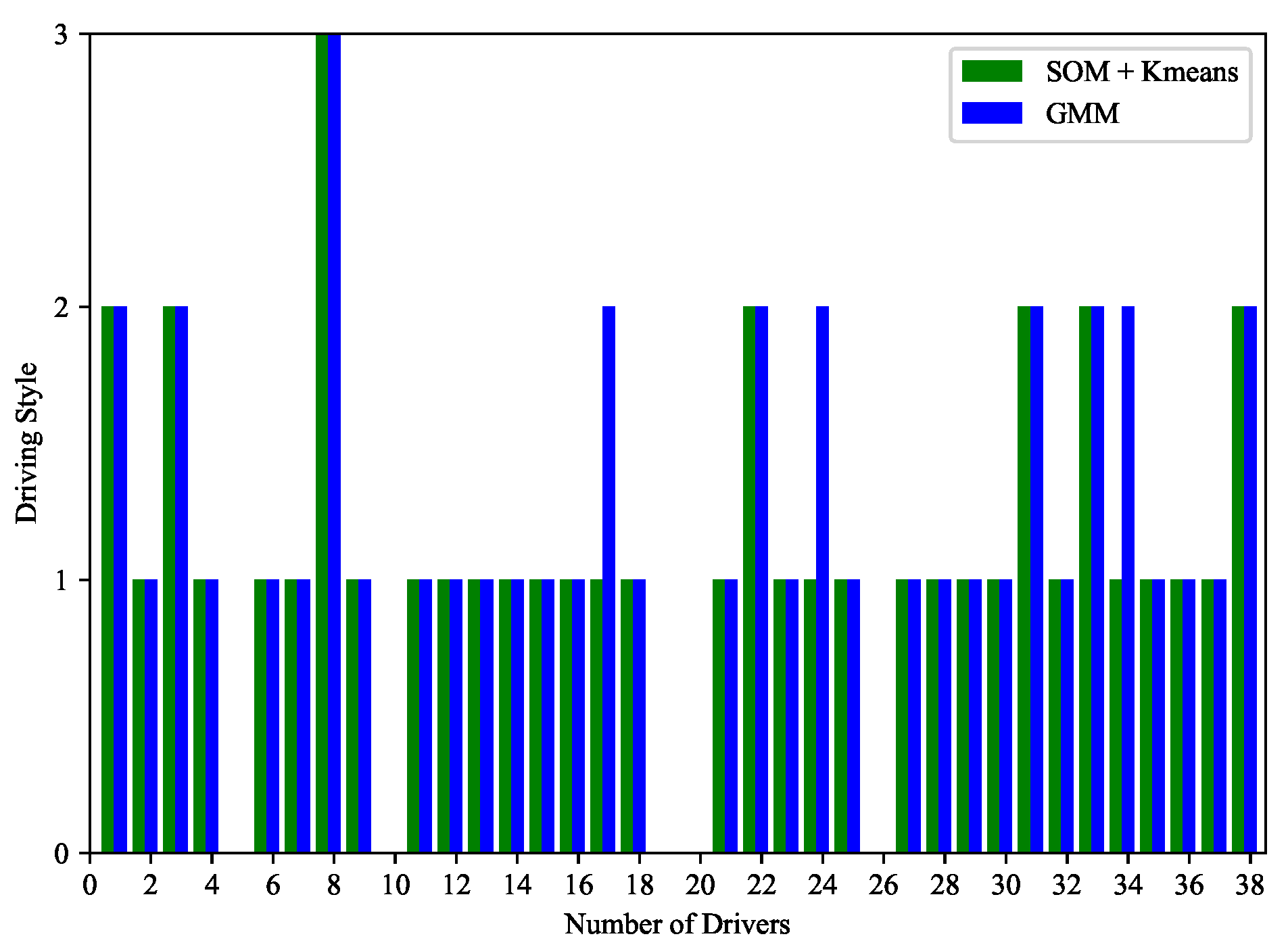
• The style recognition experiments show that the proposed SOM+K-means model, which has the recognition consistency of 90.9% with the GMM model, is accurate enough to recognize the driving styles of different drivers.
• The comparative experiments of the vehicle speed prediction indicate that the inclusion of the driving style feature in the input enhances the overall prediction accuracy compared to the scenario without the introduction of the driving style input.
• The fuel-saving evaluation simulation reveals that the human–machine collaborative driving controller saves 3–4% more fuel than human drivers.

Moving forward, prospective research avenues may encompass the refinement and further development of the human–machine collaborative methodology, as well as exploring the application of nonlinear MPC within the framework of the optimal controller design.

References

1. Delgado, O.; Rodríguez, F.; Muncrief, R. Fuel efficiency technology in european heavy-duty vehicles: Baseline and potential for the 2020–2030 time frame. Communications 2017, 49, 847129–848102. [Google Scholar]
2. Karlsson, I.; Rootzen, J.; Johnsson, F.; Erlandsson, M. Achieving net-zero carbon emissions in construction supply chains–A multidimensional analysis of residential building systems. Dev. Built Environ. 2021, 8, 100059. [Google Scholar] [CrossRef]
3. Li, H.; Zhu, D.; Shang, L.; Fan, P. Research on an energy management strategy and energy optimisation of hydraulic hybrid power mining trucks. Int. J. Veh. Des. 2021, 85, 246–273. [Google Scholar] [CrossRef]
4. Na, X.; Cebon, D. Quantifying fuel-saving benefit of low-rolling-resistance tyres from heavy goods vehicle in-service operations. Transp. Res. Part D Transp. Environ. 2022, 113, 103501. [Google Scholar] [CrossRef]
5. Kawajiri, K.; Kobayashi, M.; Sakamoto, K. Lightweight materials equal lightweight greenhouse gas emissions?: A historical analysis of greenhouse gases of vehicle material substitution. J. Clean. Prod. 2020, 253, 119805. [Google Scholar] [CrossRef]
6. McTavish, S.; McAuliffe, B. Improved aerodynamic fuel savings predictions for heavy-duty vehicles using route-specific wind simulations. J. Wind. Eng. Ind. Aerodyn. 2021, 210, 104528. [Google Scholar] [CrossRef]
7. Zarrinkolah, M.T.; Hosseini, V. Methane slip reduction of conventional dual-fuel natural gas diesel engine using direct fuel injection management and alternative combustion modes. Fuel 2023, 331, 125775. [Google Scholar] [CrossRef]
8. Jia, C.; Zhou, J.; He, H.; Li, J.; Wei, Z.; Li, K.; Shi, M. A novel energy management strategy for hybrid electric bus with fuel cell health and battery thermal-and health-constrained awareness. Energy 2023, 271, 127105. [Google Scholar] [CrossRef]
9. Hou, S.; Yin, H.; Pla, B.; Gao, J.; Chen, H. Real-time energy management strategy of a fuel cell electric vehicle with global optimal learning. IEEE Trans. Transp. Electrif. 2023, 16, 2645. [Google Scholar] [CrossRef]
10. Chu, H.; Guo, L.; Gao, B.; Chen, H.; Bian, N.; Zhou, J. Predictive cruise control using high-definition map and real vehicle implementation. IEEE Trans. Veh. Technol. 2018, 67, 11377–11389. [Google Scholar] [CrossRef]
11. Liang, J.; Feng, J.; Fang, Z.; Lu, Y.; Yin, G.; Mao, X.; Wu, J.; Wang, F. An energy-oriented torque-vector control framework for distributed drive electric vehicles. IEEE Trans. Transp. Electrif. 2023. [Google Scholar] [CrossRef]
12. Yang, L.; Bian, Y.; Zhao, X.; Ma, J.; Wu, Y.; Chang, X.; Liu, X. Experimental research on the effectiveness of navigation prompt messages based on a driving simulator: A case study. Cogn. Technol. Work. 2021, 23, 439–458. [Google Scholar] [CrossRef]
13. Rohani, M. Bus Driving Behaviour and Fuel Consumption. Ph.D. Thesis, University of Southampton, Southampton, UK, 2012. [Google Scholar]
14. Loman, M.; Šarkan, B.; Skrúcanỳ, T. Comparison of fuel consumption of a passenger car depending on the driving style of the driver. Transp. Res. Procedia 2021, 55, 458–465. [Google Scholar] [CrossRef]
15. Zhao, X.; Wu, Y.; Rong, J.; Zhang, Y. Development of a driving simulator based eco-driving support system. Transp. Res. Part C Emerg. Technol. 2015, 58, 631–641. [Google Scholar] [CrossRef]
16. Tu, R.; Xu, J.; Li, T.; Chen, H. Effective and acceptable eco-driving guidance for human-driving vehicles: A review. Int. J. Environ. Res. Public Health 2022, 19, 7310. [Google Scholar] [CrossRef] [PubMed]
17. Gonder, J.; Earleywine, M.; Sparks, W. Analyzing vehicle fuel saving opportunities through intelligent driver feedback. SAE Int. J. Passeng. Cars-Electron. Electr. Syst. 2012, 5, 450–461. [Google Scholar] [CrossRef]
18. Xing, Y.; Lv, C.; Cao, D.; Hang, P. Toward human-vehicle collaboration: Review and perspectives on human-centered collaborative automated driving. Transp. Res. Part C Emerg. Technol. 2021, 128, 103199. [Google Scholar] [CrossRef]
19. Marcano, M.; Díaz, S.; Pérez, J.; Irigoyen, E. A review of shared control for automated vehicles: Theory and applications. IEEE Trans. Hum.-Mach. Syst. 2020, 50, 475–491. [Google Scholar] [CrossRef]
20. Kowol, P.; Nowak, P.; Banaś, W.; Bagier, P.; Lo Sciuto, G. Haptic Feedback Remote Control System for Electric Mechanical Assembly Vehicle Developed to Avoid Obstacles. J. Intell. Robot. Syst. 2023, 107, 41. [Google Scholar] [CrossRef]
21. Noubissie Tientcheu, S.I.; Du, S.; Djouani, K. Review on Haptic Assistive Driving Systems Based on Drivers’ Steering-Wheel Operating Behaviour. Electronics 2022, 11, 2102. [Google Scholar] [CrossRef]
22. Liu, J.; Dai, Q.; Guo, H.; Guo, J.; Chen, H. Human-oriented online driving authority optimization for driver-automation shared steering control. IEEE Trans. Intell. Veh. 2022, 7, 863–872. [Google Scholar] [CrossRef]
23. Erlien, S.M.; Fujita, S.; Gerdes, J.C. Shared steering control using safe envelopes for obstacle avoidance and vehicle stability. IEEE Trans. Intell. Transp. Syst. 2015, 17, 441–451. [Google Scholar] [CrossRef]
24. Chu, H.; Guo, L.; Yan, Y.; Gao, B.; Chen, H. Self-learning optimal cruise control based on individual car-following style. IEEE Trans. Intell. Transp. Syst. 2021, 22, 6622–6633. [Google Scholar] [CrossRef]
25. Chu, H.; Zhuang, H.; Wang, W.; Na, X.; Guo, L.; Zhang, J.; Gao, B.; Chen, H. A Review of Driving Style Recognition Methods From Short-Term and Long-Term Perspectives. IEEE Trans. Intell. Veh. 2023. [Google Scholar] [CrossRef]
26. Lian, J.; Wang, X.r.; Li, L.h.; Zhou, Y.f.; Yu, S.z.; Liu, X.j. Plug-in HEV energy management strategy based on SOC trajectory. Int. J. Veh. Des. 2020, 82, 1–17. [Google Scholar] [CrossRef]
27. Zhang, B.; Yu, W.; Jia, Y.; Huang, J.; Yang, D.; Zhong, Z. Predicting vehicle trajectory via combination of model-based and data-driven methods using Kalman filter. Proc. Inst. Mech. Eng. Part D J. Automob. Eng. 2023, 09544070231161846. [Google Scholar] [CrossRef]
28. Ammoun, S.; Nashashibi, F. Real time trajectory prediction for collision risk estimation between vehicles. In Proceedings of the 2009 IEEE 5th International Conference on Intelligent Computer Communication and Processing, Cluj-Napoca, Romania, 27–29 August 2009; pp. 417–422. [Google Scholar]
29. Shen, H.; Wang, Z.; Zhou, X.; Lamantia, M.; Yang, K.; Chen, P.; Wang, J. Electric Vehicle Velocity and Energy Consumption Predictions Using Transformer and Markov-Chain Monte Carlo. IEEE Trans. Transp. Electrif. 2022, 8, 3836–3847. [Google Scholar] [CrossRef]
30. Daugherty, P.R.; Wilson, H.J. Human + Machine: Reimagining Work in the Age of AI; Harvard Business Press: Boston, MA, USA, 2018. [Google Scholar]
31. Liu, J.; Guo, H.; Song, L.; Dai, Q.; Chen, H. Driver-automation shared steering control for highly automated vehicles. Sci. China Inf. Sci. 2020, 63, 63. [Google Scholar] [CrossRef]
32. Mosharafian, S.; Razzaghpour, M.; Fallah, Y.P.; Velni, J.M. Gaussian process based stochastic model predictive control for cooperative adaptive cruise control. In Proceedings of the 2021 IEEE Vehicular Networking Conference (VNC), Ulm, Germany, 10–12 November 2021; pp. 17–23. [Google Scholar]
33. Mulder, M.; Abbink, D.A.; Boer, E.R. Sharing control with haptics: Seamless driver support from manual to automatic control. Hum. Factors 2012, 54, 786–798. [Google Scholar] [CrossRef]
34. Brandt, T.; Sattel, T.; Bohm, M. Combining haptic human-machine interaction with predictive path planning for lane-keeping and collision avoidance systems. In Proceedings of the 2007 IEEE Intelligent Vehicles Symposium, Istanbul, Turkey, 13–15 June 2007; pp. 582–587. [Google Scholar]
35. Li, R.; Li, Y.; Li, S.E.; Burdet, E.; Cheng, B. Driver-automation indirect shared control of highly automated vehicles with intention-aware authority transition. In Proceedings of the 2017 IEEE Intelligent Vehicles Symposium (IV), Angeles, CA, USA, 11–14 June 2017; pp. 26–32. [Google Scholar]
36. Flemisch, F.; Heesen, M.; Hesse, T.; Kelsch, J.; Schieben, A.; Beller, J. Towards a dynamic balance between humans and automation: Authority, ability, responsibility and control in shared and cooperative control situations. Cogn. Technol. Work. 2012, 14, 3–18. [Google Scholar] [CrossRef]
Figure 1. The overall architecture of the proposed fuel-saving-oriented collaborative driving system.
Energies 16 06163 g001
Figure 2. Fixed route between Shanghai and Xuchang.
Energies 16 06163 g002
Figure 3. The clustering process of SOM and K-means.
Energies 16 06163 g003
Figure 4. The results of driving style recognition: the numbers 1, 2, and 3 represent conservative, moderate, and aggressive driving styles, respectively.
Energies 16 06163 g004
Figure 5. Structure of LSTM network.
Energies 16 06163 g005
Figure 6. Fitting performance in data normalization: (a) fuel consumption rate, (b) model residuals.
Energies 16 06163 g006
Figure 7. Vehicle speed prediction under different input features. (a) S1; (b) S2; (c) S3; (d) S4.
Energies 16 06163 g007
Figure 8. Partial enlarged view of Figure 7: from 7400 s to 7500 s. (a) S1; (b) S2; (c) S3; (d) S4.
Energies 16 06163 g008
Figure 9. Prediction error varies with prediction step for different input features. (a) RMSE; (b) MAPE.
Energies 16 06163 g009
Figure 10. Effect of driving style on velocity prediction.
Energies 16 06163 g010
Figure 11. Profile of the real-world driving speed.
Energies 16 06163 g011
Figure 12. Probability distribution graphs of the vehicle speed.
Energies 16 06163 g012
Figure 13. Comparison result in the high-speed range.
Energies 16 06163 g013
Figure 14. Comparison result in the medium-speed range.
Energies 16 06163 g014