Electrostatic Field for Positive Lightning Impulse Breakdown Voltage in Sphere-to-Plane Air Gaps Using Machine Learning

Abstract

Breakdown (BD) voltage is significant in high-voltage power electric machines. Currently, BD voltages are mainly predicted by the semi-empirical formula in strongly inhomogeneous electric fields. However, the equation could not be applied for electrodes with weakly inhomogeneous electric fields. In this paper, positive lightning impulse BD voltages are predicted in various sphere-to-plane air gaps using forms of machine learning such as support vector regression (SVR), Bayesian regression (BR) and multilayer perceptron (MLP). Unlike previous studies, a method is also proposed by introducing streamer propagation characteristics as new features and by removing electric field gradients as unnecessary features to find out how to reduce the feature dimension. The streamer propagation characteristics are suggested to reflect the possibility of a discharge process between electrodes. Predicted voltages from machine learning algorithms are compared with the experimental results and calculated voltages from the semi-empirical formula. Firstly, the predictions from each model agreed well with the datasets. New features were observed to be applied for machine learning algorithms and to be as important as known electrostatic features before discharge. Secondly, predicted BD voltages were more accurate than calculated voltages from the semi-empirical equation in strongly inhomogeneous electric fields. Predictions from each model also agreed well with the experimental results in weakly inhomogeneous electric fields. The prediction accuracy of SVR was better than those of BR and MLP. Machine learning algorithms were also shown to be applied for electrodes with a wide range of inhomogeneities, unlike a semi-empirical method. We expect that the suggested features and machine learning algorithms can be used for accurately calculating BD voltages.

1. Introduction

Dielectric design of electric equipment is to predict the breakdown voltage. Electric field distribution of an air gap has an influence on its dielectric strength [1]. In strongly inhomogeneous field distributions (radius $\ll$ gap distance) such as needle-to-plane, air dielectric insulation strength is mainly dependent on either the maximum electric field or streamer propagation characteristics. However, electrical breakdown becomes complex in weakly inhomogeneous field distribution (radius $\le$ gap distance).

Many studies have sought to predict the electrical breakdown by using q particle-in- cell method, a fluid model, an air discharge mechanism and machine learning. The particle-in-cell method is applied to gaps less than tens of um at pd lower than Paschen’s minimum to predict minimum ignition voltages in the circuit breaker. The fluid model also shows that it is possible to model electrical breakdown of air at pd values higher than Paschen’s minimum [2,3]. Various methods are suggested to predict the breakdown voltage of air gaps with a typical electrode [4,5,6,7,8,9]. However, more research is required to solve several concerns [10]. Recently, streamer process during discharge has been studied to calculate the breakdown voltage. It involves the inception and propagation, which are determined by the ratio between positive electrode shape and gap distance in inhomogeneous electric fields [11]. This method is still not perfect and can mainly be used to calculate BD voltages in strongly inhomogeneous electric fields.

A neural network is applied to predict electrical breakdown voltages of transformer oil or to evaluate partial discharge in transformer oil [12,13,14]. Neural network is mainly used to precisely analyze the performance of the complex system, which involves various materials, such as pure oils, water contents, impurities and solid insulators. A support vector machine (SVM) is utilized to predict BD voltages of the air in various electrodes, such as rod-to-plane and sphere-to-sphere [15,16,17]. Generic algorithm (GA) and least square algorithm are applied for the feature selection [18,19]. Previous studies consider electrostatic field features which characterize electrode shapes before discharge. However, it is impossible for such inputs to represent the discharge process after ignition. Some of these features may also not be useful. Thus, in this paper, a method is suggested by introducing streamer propagation characteristics as new features and by removing electric field gradients as unnecessary features. Unlike former studies, electrostatic field features are calculated based on the electric field that exceeds 90% of the maximum electric field. Machine learning algorithms are also investigated to apply for inhomogeneous electric fields with various nonuniformities.

Electric fields change during the discharge. The complete breakdown takes place when the electric fields stay sufficiently large during the discharge. Thus, streamer propagation characteristics are considered to represent the possibility of the sustainable discharge process between electrodes. If we involve electrostatic fields before discharge and streamer propagation characteristics at the same time, it may be possible to predict the BD voltage more accurately. For this, various electrostatic fields before discharge are calculated to characterize the capacitive energy and inhomogeneity of each gap structure. Streamer propagation characteristics are also expressed as the ratio of electric fields over the critical electric field for streamer propagation. These features are utilized as inputs of machine learning to calculate the electrical BD voltage. Machine learning is necessary for automating the entire electrical breakdown analysis processes based on automatic electric field calculations. In particular, SVR and Bayesian regression can train models even with a small amount of data. Computational efficiency of two algorithms is high, so that these algorithms draw results within a short time, as shown in self-driving applications [20]. SVR and Bayesian regression are also compared with a multilayer perceptron (MLP) neural network.

In this paper, positive lightning impulse BD voltage is predicted by SVR and Bayesian regression and MLP in a sphere-to-plane electrode with air gaps of <200 mm. Predicted BD voltages from machine learning are compared with both experimental results and calculated voltages in the strongly inhomogeneous electric fields. Moreover, prediction accuracy of BD voltages is analyzed in weakly inhomogeneous electric fields. Section 2 presents the limits of the semi-empirical method and the need for machine learning. In Section 3, suggested parameters are defined as new features, and electrostatic features are expressed. Section 4 explains machine learning algorithms and parameter tunning. Section 5 provides experimental BD results to make datasets for machine learning. In Section 6, simulation results are discussed. Section 7 gives the conclusion of this paper.

2. Semi-Empirical Methods for BD Voltage and Necessity of Machine Learning

Air insulation design criteria are mainly based on semi-empirical methods related to streamer inception and propagation. Firstly, the streamer breakdown criterion is known for calculating inception voltages or breakdown voltages in inhomogeneous electric fields under various gases [21]. The criterion is expressed by Equation (1); $x_c$ is either identical with the gap distance or a critical avalanche length; K is the number of critical electrons, which is required for electrical breakdown; α is the ionization coefficient. K and α are influenced by various factors, such as humidity, air density, gas mixture ratio and electrode shape [22,23].

$${\int }_0^{x_c}\alpha dx=K$$

(1)

Secondly, a streamer propagates between electrodes in case the applied voltage is large enough to sustain the propagation process [24]. Semi-empirical Equation (2) for the BD voltage is expressed by the voltage drop of streamer head and propagation length; in (2), d is the distance between electrodes in mm, $E_{st}$ is the internal field strength along the positive ion channels behind the head $\mathrm{a}\mathrm{n}\mathrm{d} U_0$ is the equivalent potential required for ionization; it is approximately 20–45 kV [25,26]. (Calculated voltages from (2) are compared with predicted voltages from machine learning in strongly inhomogeneous fields).

$$U_b=E_{st}·d+U_0$$

(2)

These equations are only used in case either gap distances or electrode shapes satisfy certain conditions; (1) can be applied to weakly inhomogeneous electric fields’ needle-plane or sphere-plane; (2) can be used in strongly inhomogeneous electric fields. Incorrect ionization coefficients (α) and improper K value cause the error in calculated BD voltages from (1). Breakdown in ambient air is also influenced by metallic particles and protrusion, which cause the distortion of the electric field [27,28]. However, these are not involved in semi-equations. Thus, machine learning is necessary for finding non-linear relationships between multiple variables and BD voltages through the kernel function of SVR or hidden layer of MLP. Moreover, machine learning quantifies the effect of each variable over BD voltages in detail, and it is possible to categorize variables affecting BD voltages in each sphere-to-plane air gap. Thus, machine learning predicts BD voltages with only accurate variables related to electrode shapes, except for inaccurate data. This makes machine learning apply to various electrode shapes.

3. Electrostatic Fields as Input Parameters for Machine Learning

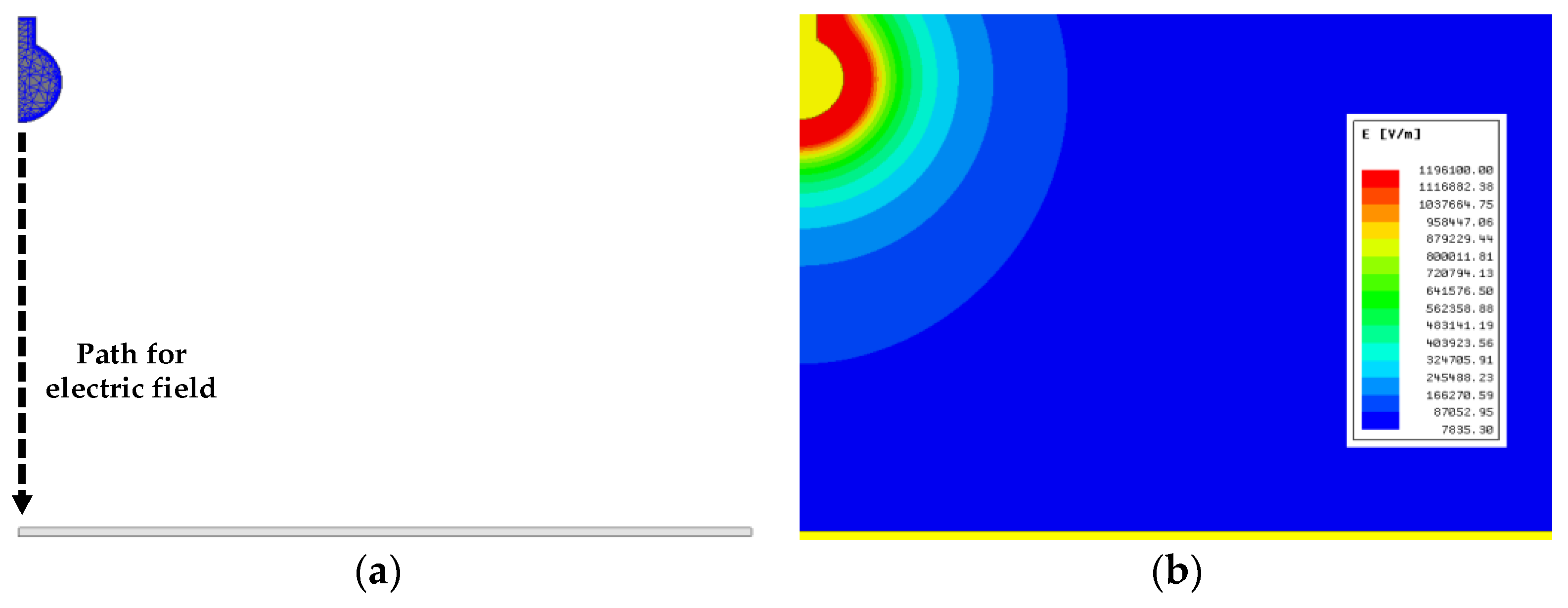
3.1. Electric Fields Properties of Sphere-to-Plane Electrodes

As shown in Figure 1, the electric field between electrodes is calculated along the shortest path with MAXWELL software (ANSYS MAXWELL 19 version). A voltage of 1 kV is applied to each sphere, and the ground potential is applied to the plane electrode.

Electric field distribution and the nonuniformity coefficient (NUC) are shown in Figure 2. Maximum electric field is inversely proportional to the radius. Electric fields are exponentially varying with respect to gap distances. As radius decreases, the electric field gradient increases around sphere electrodes. Nonuniformity coefficients range from 4.7 to 73 in all the test electrodes. In the case of a radius of 3 mm, the slope of NUC is much larger than that of other sphere electrodes. As radius increases from 3 to 10 mm, the slope rapidly decreases. Strongly inhomogeneous electric fields are shown in sphere-to-plane air gaps of 3 mm radius. Inhomogeneity is not large for spheres of radius 10 and 25 mm.

3.2. Suggested Input Features: Streamer Propagation Characteristics

A positive streamer triggers an electrical BD in a nonuniform field with a positive polarity if the air gap is <200 mm [29]. The critical electric field for steamer penetration in the gap is 0.4–0.5 kV/mm, with a standard deviation of approximately 3% under standard atmospheric conditions [30,31]. The probability of electrical BD increases as either the average electric field between electrodes or the electric field of the plane electrode approaches the critical electric field. Thus, the ratios of either the average electric field over the critical electric field or electric field of the plane electrode over the critical electric field are used as input parameters to represent streamer propagation characteristics.

3.3. Electrostatic Fields as Input Parameters

Electrostatic fields for machine learning are listed in

Table 1. Electrostatic fields.

Parameter	Notation
Field distribution	$E_{max},E_{std}$
Capacitive characteristics	$E_s,E_{s ave}$
Streamer propagation characteristics	$\frac{E_{ave}}{E_{c0}},\frac{E_g}{E_{c0}}$
Inhomogeneity	${V\_E}_{90},{L\_E}_{90},E_s\_E_{90}, V_r\_E_{90}, L_r\_E_{90}$

. Eleven physical quantities are calculated and then classified into four groups. The maximum electric field ($E_{max}$) and the electric field deviation ($E_{std}$) are fundamental features in electrode systems. The capacitive characteristics involve the stored energy ($E_s$) and the stored average energy in the air gap ($E_{s ave}$). Streamer propagation characteristics are considered to represent the probability that a streamer penetrates between the sphere and the plane electrode. Inhomogeneity is a measure of nonuniformity imparted by variations in either the radius of the sphere or the gap distance.

Eleven input parameters are defined at the point of the maximum electric field or along the path with an electric field that exceeds 90% of the maximum field. These parameters are expressed as follows:

1.

Maximum electric field: $E_{max}$

$$E_{max}=\max E_i (i=1, 2, 3, \dots , n),$$

(3)

where $E_i$ is the electric field of the i-th element and n is the sum of elements in the shortest path;

2.

Electric field standard deviation: $E_{std}$

$$E_{std}=\sqrt{\frac{1}{n}{\sum }_{i=1}^n{\left(E_i-E_{ave}\right)}^2},$$

(4)

$$E_{ave}={\sum }_{i=1}^n\frac{E_i}{n},$$

(5)

where $E_{std}$ is calculated along the shortest path and $E_{ave}$ is the average electric field;

3.

Energy stored along the shortest path in the air gap: $E_s$

$$E_s={\sum }_{i=1}^n{E}_i^2 d_i,$$

(6)

where $d_i$ is the fine distance of the i-th element and $E_s$ is the energy stored along the shortest path. $E_s$ is dependent on the electrode shape; stored energy tends to become concentrated around the sphere owing to the nonuniformity;

4.

Average energy stored along the shortest path in the air gap: $E_{s ave}$

$$E_{s ave}=\frac{E_s}{n} ,$$

(7)

where $E_i$ is the electric field of the i-th element and n is the sum of elements in the shortest path;

5.

Ratio of the average electric field to the critical electric field: $C_1$

$$C_1=\frac{E_{ave}}{E_{c0}} ,$$

(8)

where $E_{c0}$ is 0.5 kV/mm (the critical electric field for streamer propagation);

6.

Ratio of the plane electrode electric field to the critical electric field: $C_2$

$$C_2=\frac{E_g}{E_{c0}},$$

(9)

where $E_{c0}$ is 0.5 kV/mm (the critical electric field for streamer propagation). $E_g$ is the electric field of the plane electrode;

7.

Voltage drop: $V\_E_{90}$

$$V\_E_{90}=\sum E_i d_i, \mathrm{where} E_i\ge E_{max}\times 0.9,$$

(10)

where $V\_E_{90}$ is the voltage drop in the region with an electric field strength that exceeds 90% of the strength present with the maximum electric field;

8.

Path length: $L\_E_{90}$

$$L\_E_{90}=\sum d_i, \mathrm{where} E_i\ge E_{max}\times 0.9,$$

(11)

where $L\_E_{90}$ considers the ionization and avalanche formation that precedes streamer inception and is the sum of the fine distances;

9.

Energy stored in the region where the field exceeds 90% of the maximum field: $E_s\_E_{90}$

$$E_s\_E_{90}=\sum E_i^2{d}_i, \mathrm{where} E_i\ge E_{max}\times 0.9;$$

(12)

10.

Path length that stores 90% of the total energy stored along the shortest path: ${L\_E}_{s90}$

$$L\_E_{s90}=\sum d_i, \mathrm{where} \sum E_i^2 d_i\ge E_s\times 0.9;$$

(13)

11.

Relative ratio of the voltage to the length: $V_r\_E_{90}$, $L_r\_E_{90}$

$$V_r\_E_{90}=\frac{V\_E_{90}}{V} .$$

(14)

$$L_r\_E_{90}=\frac{L\_E_{90}}{d} .$$

(15)

4. Machine Learning Algorithms and Parameter Tunning

4.1. Support Vector Regression

An SVM is a machine-learning algorithm. An SVR is an SVM that solves regression problems. An $\epsilon$-SVR identifies the hyperplane on which the loss range ($\epsilon$) is acceptable; the soft margin is indicated by a slack variable ($\xi$). The primary optimization problem addressed by an $\epsilon$-SVR is the problem represented in (16). $C$ and $\epsilon$ serve as hyperparameters that enhance the accuracies of the predicted values [16,17]:

$$min\frac{1}{2}{\parallel \omega \parallel }^2+C {\sum }_{i=1}^m({\xi }_i-{\xi }_i^{*}).$$

(16)

$$\mathrm{s}. \mathrm{t}. f\left(x_i\right)-y_i \le \epsilon +{\xi }_i.$$

(17)

$$y_i-f\left(x_i\right)\le \epsilon +{\xi }_i^{*}.$$

(18)

$${\xi }_i,{\xi }_i^{*}\ge 0 (i=0, 1, 2, 3\dots n).$$

(19)

$\epsilon$-SVR is a convex quadratic problem, but it can be converted to a dual problem. The decision function of $\mathrm{t}\mathrm{h}\mathrm{e} \epsilon$-SVR is defined in (20). The radial basis function serves as the kernel that maps values from the original space to higher dimensions, and thus arranges the data in a linear manner. $\gamma$ is a parameter of the kernel function, comprising the Euclidean distance between two points:

$$f\left(x\right)={\sum }_{i=1}^m({\alpha }_i^{*}-{\alpha }_i)K(x,x_i)+b.$$

(20)

$$K\left(x,x_i\right)=\exp \left(-\gamma {\parallel x_i-x_j\parallel }^2\right).$$

(21)

4.2. Bayesian Regression

Bayesian models are utilized in various fields, such as artificial intelligence and machine learning. Bayes’ Theorem connects the prior probability and the posterior probability. Its Equation (22) is as follows [32]:

$$p\left(\theta |E\right)=\frac{p\left(E\right|\theta \left)p\right(\theta )}{ p\left(E\right)},$$

(22)

where $\theta$ is a parameter to be estimated, $p\left(\theta \right)$ is the prior probability of $\theta$, E is data and $p\left(E\right)$ is a constant value. $p\left(E|\theta \right)$ is the likelihood. Bayesian inference uses prior probability and likelihood to estimate the posterior probability, which is Equation (23) [28,29]:

$$\left(x|E\right)={\int }_0^{x}p\left(x|\theta \right)p\left(\theta |E\right)d\theta .$$

(23)

This equation shows that the posterior probability keeps changing with new data. Since posterior probabilities can be used as new prior probabilities, data inference automation is possible.

The Bayesian regression uses Bayesian inference (conditional probability) for regression analysis between target ($Y$) and independent variables ($X$). The formula of Bayesian regression is (24) [33]; X consists of n attributes such as $x_1, x_2,\dots \mathrm{a}\mathrm{n}\mathrm{d} x_n$; each attribute is assumed to be independent; $Y$, $X$ and $ϵ$ are random variables; $ϵ$ is a singular value. The hyperparameters are found by GridSearch.

$$Y=a+bX\left[n\right]+ϵ\left[n\right].$$

(24)

4.3. Multilayer Perceptron Neural Networks

Multilayer perceptron (MLP) neural network is a supervised learning algorithm in breakdown analysis [34]. Given a set of input parameters ($X$ = $X_1, X_2,\dots$,$X_3$) and a target ($Y$), it can learn a model for regression. Figure 3 shows the conceptual multilayer perceptron for predicting BD voltages. MLP is a two layers model, which consists of an input layer, one hidden layer and an output layer.

The input layer consists of a set of neurons representing input parameters. Each neuron in the hidden layer transforms the values from the previous layer with a weighted linear summation ($W_1{X}_1+W_2{X}_2+...+W_m{X}_m$), followed by the activation function. The output layer receives values from the hidden layer and transforms them into the output values. In a neuron of one hidden layer, MLP learns Equation (25). $W_1 \mathrm{a}\mathrm{n}\mathrm{d}{W}_2$ are the weights of the input layer and hidden layer. $b_1 \mathrm{a}\mathrm{n}\mathrm{d}{b}_2$ are the bias added to the hidden layer and the output layer. $g$ is the activation function and the identity function is used. The solver uses ‘lbfgs’. The number of neurons in one hidden layer is found by GridSearch.

$$f\left(x\right)=W_{2}g\left(W_1^{T}x+b_1\right)+b_2.$$

(25)

4.4. Feature Normalization and Parameter Tunning

The input parameters are normalized to eliminate the value deviation and unit effects; this normalization improves machine learning performance. The input parameters are normalized using (26):

$$X_i=\frac{x_i-x_{min}}{x_{max}-x_{min}},$$

(26)

where $X_i$ is the normalized value of the input parameter ($x$); $x_{min} \mathrm{a}\mathrm{n}\mathrm{d} x_{max}$ are the minimum and maximum values, respectively.

$K$-fold cross-validation is used, considering the limited amount of data. $K$ is 3. A test dataset involves nine samples, which are randomly divided into three sub-datasets; two of these sub-datasets are used to train each SVR, the Bayesian regression model and MLP, whereas the remaining sub-datasets are used to validate models. GridSearch was used to select the hyperparameters and tune the model.

5. Breakdown Experimental Results for Dataset Design

The experimental setup to predict lightning impulse BD voltages was shown in Figure 4. This setup involved an impulse generator, electrodes and measurement systems. The generator delivered 1.2/50-$\mathsf{\mu }\mathrm{s}$ standard impulses. Measurement systems stored voltage waveforms in an oscilloscope and a personal computer; measured voltages were derived from the voltage divider. BD experiments were conducted in an up-and-down method. BD voltages were measured 15 times under each condition. Calculated BD voltages were mean values, except for maximum and minimum voltages.

Nonuniformity coefficients (NUC) were evaluated to indicate nonuniform degrees of sphere-to-plane air gaps. Mean BD voltages and calculated NUC were shown in

Table 2. Mean BD voltages and nonuniformity coefficients for datasets.

Gap [mm]	Radius 3 mm			Radius 10 mm			Radius 25 mm
	Number	NUC	${\mathit{V}}_{\mathit{B}\mathit{D}}$	Number	NUC	${\mathit{V}}_{\mathit{B}\mathit{D}}$	Number	NUC	${\mathit{V}}_{\mathit{B}\mathit{D}}$
70	1	20.044	70.71	13	11.032	82.67	25	7.134	104.21
80	2	33.126	79.57	14	13.886	95.10	26	7.375	110.00
90	3	34.118	84.10	15	14.479	99.24	27	7.535	115.65
100	4	36.833	90.59	16	16.091	104.52	28	7.828	122.50
110	5	39.268	96.93	17	18.009	113.49	29	8.077	127.74
120	6	42.177	103.14	18	18.858	119.84	30	8.172	131.78
130	7	44.185	109.20	19	19.933	125.42	31	8.530	140.47
140	8	46.522	115.13	20	19.963	128.00	32	8.570	148.17
150	9	48.685	120.91	21	20.976	135.03	33	8.645	153.84
160	10	49.861	126.56	22	20.833	137.29	34	8.686	162.14
170	11	51.936	132.07	23	22.587	142.32	35	9.209	167.85
180	12	55.647	138.37	24	23.172	145.67	36	9.365	174.50

. NUC ranged from 7.134 to 55.647. Three samples in each electrode were uniformly and randomly extracted by considering NUC. Each dataset consisted of 9 samples.

$$\mathrm{Nonuniform} \mathrm{coefficients} (\mathrm{NUC})=\frac{E_{max}}{U/d}.$$

(27)

6. Model Learning and Simulation Results

6.1. Model Learning and Testing

Good datasets were important for the enhancement of machine learning accuracy. Four groups of datasets were randomly made by NUC, as shown in

Table 3. Datasets and sizes.

Dataset	Size	Sample Number
1	9	1, 5, 9, 13, 17, 21, 25, 29, 33
2		2, 6, 10, 14, 18, 22, 26, 30, 34
3		3, 7, 11, 15, 19, 23, 27, 31, 35
4		4, 8, 12, 16, 20, 24, 28, 32, 36

. The samples in all the datasets were unique. Datasets were randomly selected to learn SVR, Bayesian regression and MLP models; one of four datasets was utilized to learn models; other datasets were applied to analyze the prediction accuracy.

6.2. Comparision among Predicted Voltages, Experimental Results and Calculated Voltages

Three error indices are applied to evaluate predicted voltages: root mean square error (RMSE), mean absolute percentage error (MAPE) and relative error (RE). RMSE is expressed by (28). MAPE is given by (29). Relative Error (RE) is the individual difference.

$$RMSE=\sqrt{\frac{1}{n}{\sum }_{i=1}^n{(U_{bi}-U_{pi})}^2}.$$

(28)

$$MAPE=\frac{1}{n}{\sum }_{i=1}^n\left|\frac{U_{bi}-U_{pi}}{U_{bi}}\right|.$$

(29)

$$\mathrm{RE}=\left|\frac{U_{bi}-U_{pi}}{U_{bi}}\right|,$$

(30)

where $U_{bi}$ is the BD voltage and $U_{pi}$ is the value predicted by SVR, Bayesian regression and MLP. $n$ is the number of samples.

The error indices of four predictions were shown in

Table 4. Error indices of four predictions and comparison among SVR, BR and MLP.

Dataset	SVR		Bayesian Regression		MLP
	RMSE	MAPE	RMSE	MAPE	RMSE	MAPE
1	3.798924	0.019375	4.953797	0.028971	4.04539	0.030774
2	3.189483	0.022808	3.756385	0.024334	3.070613	0.020285
3	2.43982	0.016417	4.062541	0.023871	2.251325	0.014967
4	2.204422	0.014137	1.711295	0.008754	1.531138	0.007939

. Predictions from each model showed good agreement with the experimental results. In the case of SVR, the maximum and minimum RMSE between predictions and a corresponding dataset were about 3.79 and 2.2 kV, and MAPEs were all <2.28%. The maximum and minimum RMSE between predictions from Bayesian regression and a dataset were about 4.95 and 1.71 kV. MAPEs were all <2.89%. The maximum RMSE of MLP was higher than that of SVR, while it was lower than that of Bayesian regression. The prediction accuracy of Bayesian regression was the lowest among three algorithms, based on RMSE and MAPE.

The predicted BD voltages from SVR, Bayesian regression and MLP were compared with both experimental results and calculated voltages in a strongly inhomogeneous electric field with spheres of 3 mm radius, as shown in Figure 5. The predictions from three models exhibited good agreement with the experimental results. In particular, the maximum RE between the predicted voltages from SVR and experimental results was 4.13%. Maximum RE between the predicted voltages from Bayesian regression and experimental results was 6.30%. In the case of MLP, maximum RE was 7.75%. However, the maximum RE between calculated voltages from (2) and experimental voltages was approximately 13%. Predicted BD voltages were more accurate than calculated voltages from the semi-empirical equation. There was also BD voltage difference between SVR and Bayesian regression by 2.17%. SVR was the most accurate among the three algorithms.

Predicted BD voltages from three models were compared with experimental results in a weakly inhomogeneous electric field, as shown in Figure 6. The predictions generally agreed with experimental results. As shown in Figure 6a, the REs between predicted voltages from SVR and experimental results were within 4.05%. As there was an 8.51% error at the particular gap distances, the predicted voltages from SVR were more accurate than those from Bayesian regression. In a weakly inhomogeneous electric field with a sphere of radius 25 mm as shown in Figure 6b, REs between predicted voltages from SVR and experimental results were all <4.15%, except for a gap distance of 70 mm. In the case of predictions from Bayesian regression, REs were all <4.47%. Moreover, predicted voltages from SVR were analogous to those from MLP, except for a gap distance of 70 mm in weakly inhomogeneous electric fields.

6.3. Disucussion

Prediction of the dielectric insulation strength was challenging owing to a complex relationship between various variables and the breakdown. Nevertheless, predictions from machine learning algorithms were shown to be similar to the datasets. As new features, streamer propagation characteristics were as important as known electrostatic features characterizing electrode shapes before discharge. Electric field gradients were unnecessary due to the time-varying Poisson’s electric field during the discharge process. Suggested features were effective for lowering the feature dimension.

Three machine learning algorithms agreed well with the experimental results in all the test electrodes. In particular, predicted voltages were more precise than calculated results in range 80 mm–110 mm. SVR was more precise than MLP, which was easier to analyze than more complex systems by controlling the number of hidden layers. This showed that SVR as well as MLP could be sufficiently possible for analyzing breakdown voltages of a single medium with various factors, such as dust, salt and metallic particles. Prediction accuracy of Bayesian regression was lower than that of SVR and MLP. This was because variables affecting BD were dependent to some extent.

As there are no dominant equations for the physical discharge process under various conditions, more study is needed to confirm whether the suggested method and machine learning algorithms are applied for compressed single gas systems as well as insulator creepage structures, which are utilized in high-voltage power apparatuses.

7. Conclusions

In this paper, machine learning algorithms were investigated for predicting positive lightning impulse BD voltages in sphere-to-plane electrode systems with various nonuniformities. A method was also suggested by introducing streamer propagation characteristics as new features and by removing electrostatic field gradients as unnecessary features, to reduce feature dimensions for three algorithms, which were SVR, Bayesian regression and MLP neural network. These algorithms were trained based on new features during the discharge process and known electrostatic features characterizing electrode shapes before discharge. The predicted voltages from each model were compared with experimental results and calculated voltages from the semi-empirical equation:

(1)

The maximum RMSE between predictions from SVR and datasets was 3.79 kV, while maximum RMSEs between predictions from other models (Bayesian regression, MLP) and datasets were 4.95 kV and 4.04 kV, respectively. The predictions agreed well with the datasets. The suggested method was observed to be effective for learning models. These results also showed that streamer propagation characteristics during discharge were as important as known electrostatic features before discharge;

(2)

Predicted BD voltages from each model were more accurate than calculated voltages from the semi-empirical equation in strongly inhomogeneous electric fields with radius of 3 mm. Predictions from each model also showed agreements with experimental results in weakly inhomogeneous electric fields with spheres of 10 and 25 mm radius. Machine learning algorithms were shown to be useful for evaluating BD voltages in sphere-to-plane electrodes with a wide range of nonuniformities, unlike the semi-empirical method;

(3)

SVR was more precise than Bayesian regression and MLP under an ambient air, regardless of the nonuniformity of electrodes.

The suggested method and machine learning algorithms are expected to be applied for insulation design of air insulated switchgears (AIS) or cubic gas insulated switchgears filled with dry air or SF₆. As part of the insulation design process, predicted voltages in each electrode structure are compared with the test voltage provided by the international electronical committee (IEC) to verify the withstand performance of high-voltage power electric apparatuses. (Test voltages are dependent on operating voltages).

High-voltage power electric apparatuses have various electrode shapes, such as bare conductor electrodes, structures with the solid insulator and insulator creepage structures. Further study will be conducted for evaluating BD voltages of creepage structures under various conditions as well as dry air systems with impurities. The suggested method and machine learning algorithms will be verified for different physical situations.

References

1. Allen, L.N. Dielectric breakdown nonuniform field air gaps. IEEE Trans. Electr. Insul. 1993, 28, 183–191. [Google Scholar]
2. Klas, M.; Matejcik, S.; Radjenovic, B.; Radmilović-Radjenović, M. Experimental and theoretical studies of the breakdown voltage characteristics at micro metre separations in air. Europhys. Lett. 2011, 95, 35002. [Google Scholar]
3. Jovanovic, A.P.; Stankov, M.N.; Marković, V.L.; Stamenković, S.N. The validity of the one-dimensional fluid model of electrical breakdown in synthetic air at low pressure. Europhys. Lett. 2013, 104, 65001. [Google Scholar] [CrossRef]
4. Seeger, M.; Votteler, T.; Ekeberg, J.; Pancheshnyi, S.; Sanchez, L. Streamer and leader breakdown in air at atmospheric pressure in strongly non-uniform fields in gap less than one metre. IEEE Trans. Dielectr. Electr. Insul. 2018, 25, 2147–2156. [Google Scholar] [CrossRef]
5. Fofana, I.; Beroul, A.; Rakotonandrasana, J.-H. Application of dynamic models to predict switching impulse voltages of long air gaps. IEEE Trans. Dielectr. Electr. Insul. 2013, 20, 89–97. [Google Scholar]
6. Kim, N.K.; Lee, S.H.; Georghiou, G.; Kim, D.-W. Accurate prediction method of breakdown voltage in air at atmospheric pressure. J. Electr. Eng. Technol. 2012, 7, 97–102. [Google Scholar]
7. Arevalo, L.; Wu, D.; Jacobson, B. A consistent approach to estimate the breakdown voltage of high voltage electrodes under positive switching impulses. J. Appl. Phys. 2013, 114, 083301. [Google Scholar]
8. Prilepa, K.A.; Samusenko, A.V.; Stishkov, Y.K. Methods of calculating the air-gap breakdown voltage in weakly and strongly nonuniform fields. High Temp. 2016, 54, 655–661. [Google Scholar]
9. Klas, M.; Moravsky, L.; Matejčik, Š.; Zahoran, M.; Martišovitš, V.; Radjenović, B.; Radmilović-Radjenović, M. The breakdown voltage characteristics of compressed ambient air microdischarges from direct current to 10.2 MHz. Plasma Source Sci. Technol. 2017, 26, 055023. [Google Scholar]
10. Beroul, A.; Fofana, I. Application of the model to positive lightning discharge. In Discharge in Long Air Gap: Modeling and Applications; IOP Publishing: Bristol, UK, 2016; ISBN 978-0-7503-1236-3. [Google Scholar]
11. Pedersen, A.; Blaszczyk, A. An engineering approach to computational prediction of breakdown in air with surface charging effects. IEEE Trans. Dielectr. Electr. Insul. 2017, 24, 2775–2783. [Google Scholar]
12. Wahab, M.A.A. Artificial neural network-based prediction technique for transformer oil breakdown voltage. Electr. Power Syst. Res. 2004, 71, 73–84. [Google Scholar] [CrossRef]
13. Ghoneim, S.M.; Dessouky, S.S.; Elfaraskoury, A.A.; Sharaf, A.B.A. Prediction of insulating transformer oils breakdown voltage considering barrier effect based on artificial neural networks. Electr. Eng. 2018, 100, 2231–2242. [Google Scholar] [CrossRef]
14. Foo, J.S.; Ghosh, P.S. Artificial neural network modelling of partial discharge parameters for transformer oil diagnosis. In Proceedings of the Annual Report Conference on Electrical Insulation and Dielectric Phenomena, Cancun, Mexico, 20–24 October 2002. [Google Scholar]
15. Qiu, Z.; Ruan, J.; Huang, D.; Pu, Z. A prediction method for breakdown voltage of typical air gaps based on electric field features and support vector machine. IEEE Trans. Dielectr. Electr. Insul. 2015, 22, 2125–2135. [Google Scholar] [CrossRef]
16. Qin, Y.; Li, X.; Ren, B.; Yan, Q.; He, K. Prediction of switching impulse breakdown voltage of the air gap between tubular buses in substation. In Proceedings of the 4th International Conference on Smart Power and Internet Energy Systems, Beijing, China, 9–12 December 2022. [Google Scholar]
17. Qui, Z.; Ruan, J.; Xu, W.; Huang, C. Breakdown voltage prediction rod-plane gap in rain condition based on support vector machine. In Proceedings of the IEEE International Conference on High Voltage Engineering and Application, Chengdu, China, 19–22 September 2016. [Google Scholar]
18. Qui, Z.; Zhang, L.; Liu, Y.; Liu, J.; Hou, H.; Zhu, X. Electrostatic Field Feature Selection Technique for Breakdown Voltage Prediction of Sphere Gaps Using Support Vector Regression. IEEE Trans. Magn. 2021, 57, 7510104. [Google Scholar]
19. Qui, Z.; Hou, H.; Liao, C.; Zhu, X.; Liu, Z.; Zhang, L. An Electric Field Feature Set for Breakdown Voltage Prediction of Rod-plane Air Gaps Using Least Squares Support Vector Machine. In Proceedings of the 23rd International Conference on the Computation of Electromagnetic Field, Cancun, Mexico, 16–20 January 2022. [Google Scholar]
20. Kim, I.H.; Bong, J.H.; Park, J.Y.; Park, S.S. Prediction of driver’s intention of lane change by augmenting sensor information using machine learning techniques. Sensors 2017, 17, 1350. [Google Scholar] [CrossRef]
21. Malik, N.H. Streamer Breakdown Criterion for compressed gases. IEEE Trans. Electr. Insul. 1981, El-16, 463–467. [Google Scholar] [CrossRef]
22. Petcharaks, K. A contribuion to the streamer breakdown criterion. In Proceedings of the 11th International Symposium on High Voltage Engineering, London, UK, 27–33 August 1999. [Google Scholar]
23. Zaengl, W.S.; Petcharaks, K. Application of streamer breakdown criterion for inhomogeneous fields in dry air and SF6. In Gaseous Dielectric VII.; Springer: Berlin, Germany, 1994; pp. 153–159. [Google Scholar]
24. Christen, T.; Bohme, H.; Pedersen, A.; Blaszczyk, A. Streamer line modeling. In Scientific Computing in Electrical Engineering SCEE 2010; Springer: Berlin, Germany, 2011; pp. 173–181. [Google Scholar]
25. Meyer, H.K.; Mauseth, F.; Marskar, R.; Pedersen, A.; Blaszczyk, A. Streamer and surface charge dynamics in non-uniform air gaps with dielectric barrier. IEEE Trans. Dielectr. Electr. Insul. 2019, 26, 1163–1171. [Google Scholar] [CrossRef]
26. Pedersen, A.; Christen, T.; Blaszczyk, A.; Boehme, H. Streamer inception and propagation models for designing air insulated power devices. In Proceedings of the IEEE Conference on Electrical Insulation and Dielectric Phenomena, Virginia Beach, VI, USA, 18–21 October 2009. [Google Scholar]
27. Sarathi, R.; Krishnamurthi, M.; Reji, P. Breakdown characteristics of a short air gap with conducting particle under composite voltages. In Proceedings of the IEEE Annual Report Conference on Electrical Insulation and Dielectric Phenomena, Minneapolis, MN, USA, 19–22 October 1997. [Google Scholar]
28. Mahdy, A.M.; Anis, H.I.; Ward, S.A. Electrode roughness effects on the breakdown of air-insulated apparatus. IEEE Trans. Dielectr. Electr. Insul. 1998, 5, 612–617. [Google Scholar] [CrossRef]
29. Pigini, A.; Rizzi, G.; Garbagnati, E.; Porrino, A.; Baldo, G.; Pesavento, G. Performance of large air gaps under lightning overvoltages: Experimental study and analysis of accuracy predetermination method. IEEE Trans. Power Deliv. 1989, 4, 1379–1392. [Google Scholar] [CrossRef]
30. Morrow, R.; Lowke, L.L. Streamer propagation in air. J. Phys. D Appl. Phys. 1997, 30, 614–627. [Google Scholar] [CrossRef]
31. Rizk, F.A.M.; Trinh, G.N. Breakdown characteristics of long air gap. In High Voltage Engineering, 1st ed.; CRC Press: Boca Raton, FL, USA, 2014; pp. 223–259. [Google Scholar]
32. Frank, E.; Trigg, L.; Holmes, G.; Witten, I. Navie bayes for regression. Mach. Learn. 2000, 41, 5–25. [Google Scholar] [CrossRef]
33. Park, K.J.; Kim, T.H. Forecasting Demand of 5G Internet of things based on Bayesian Regression Model. J. Inf. Technol. Appl. Manag. 2019, 26, 61–73. [Google Scholar]
34. Bourek, Y.; M’Zou, N.; Benguesmia, H. Prediction of flashover voltage of high voltage polluted insulator using artificial intelligence. Trans. Electr. Electro. Mater. 2018, 19, 59–68. [Google Scholar] [CrossRef]
Figure 1. Electric field in sphere-to-plane air gaps for a sphere of radius 10 mm and a gap distance of 100 mm. (a) Schematic electrode; (b) electric field. (A voltage of 1 kV is applied to a sphere).
Energies 16 06221 g001
Figure 2. Electric field distributions of a function of the air gap and the radius of sphere. (a) Electric field; (b) nonuniform coefficient (NUC). (NUC = maximum electric field/average electric field).
Energies 16 06221 g002
Figure 3. Conceptual multilayer perceptron neural network. (Bias: b 1 ,   b 2 ).
Energies 16 06221 g003
Figure 4. Experimental setup.
Energies 16 06221 g004
Figure 5. Comparison between predicted voltages, calculated voltage (E_st) and experimental results in strongly inhomogeneous electric field (radius = 3 mm, VBD: Breakdown voltage). (a) SVR; (b) Bayesian regression (BR); (c) MLP.
Energies 16 06221 g005
Figure 6. Comparison between predicted voltages (from SVR, Bayesian regression and MLP) and experimental results in weakly inhomogeneous electric field (VBD: Breakdown voltage). (a,c) radius = 10 mm; (b,d) radius = 25 mm.
Energies 16 06221 g006aEnergies 16 06221 g006b