
HPPC Test Methodology Using LFP Battery Cell Identification Tests as an Example


Abstract
:1. Introduction
- An optimization-based battery cell time constant identification algorithm is implemented in software written by the authors.
- An HPPC-based method for OCV vs. SOC characteristic determination is established.
- Other contributions of the article are as follows:
- This paper gives the values of all parameters necessary to build a fully parameterized mathematical model of the cell.
- The paper explains the HPPC test development methodology step by step. In the literature, usually only the results of HPPC are given, but the process of obtaining them is not described. This paper fills that gap.
- The paper discusses potential flaws in the HPPC test results. Not every HPPC pulse recorded during measurements is suitable for further analysis and must be omitted. In the literature, this problem is hardly commented on. This paper fills that gap.
- The paper applies edge detection techniques in the analysis of the HPPC test results.
- The paper remarks on battery cell true capacity experimental estimation.
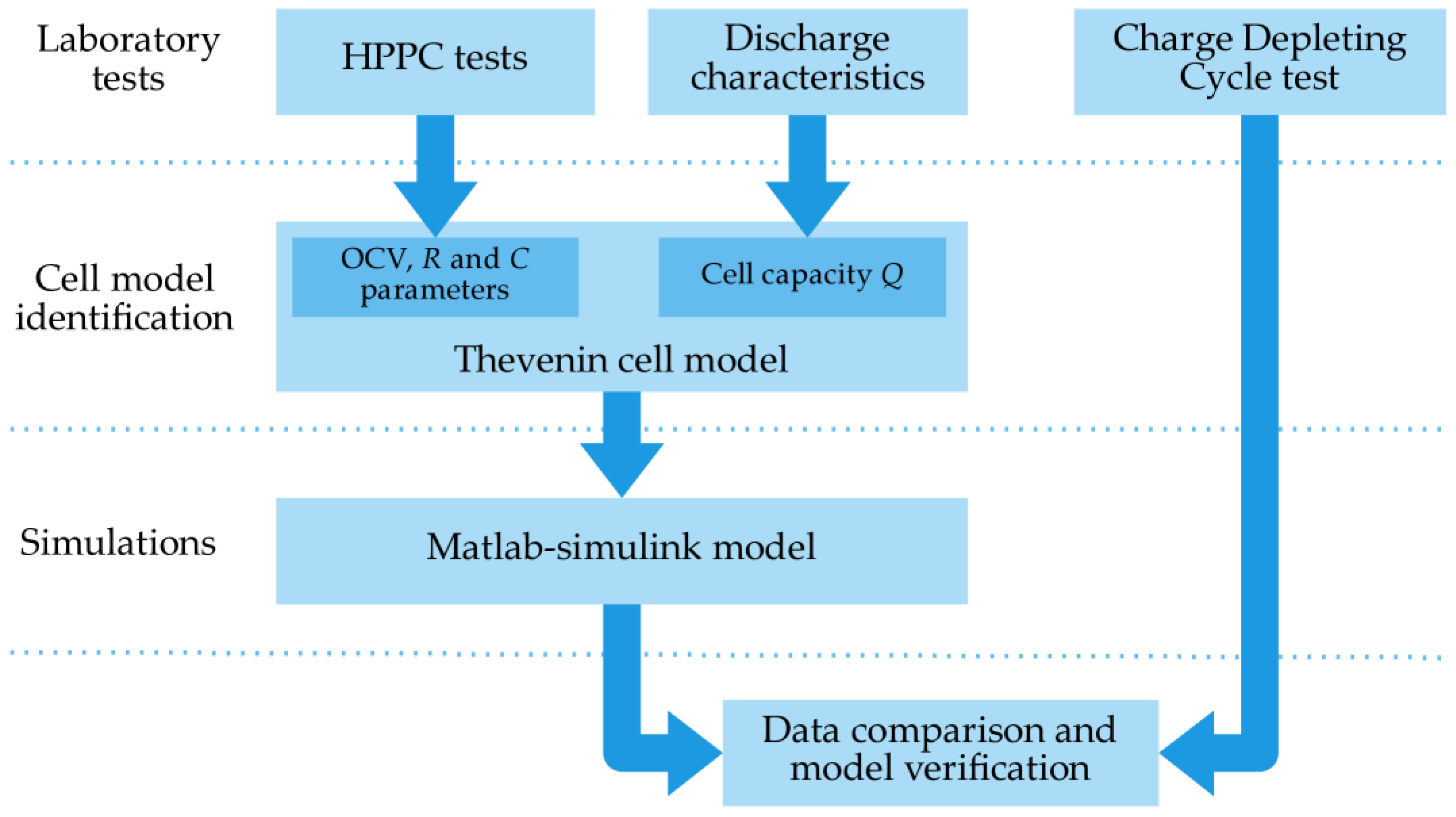
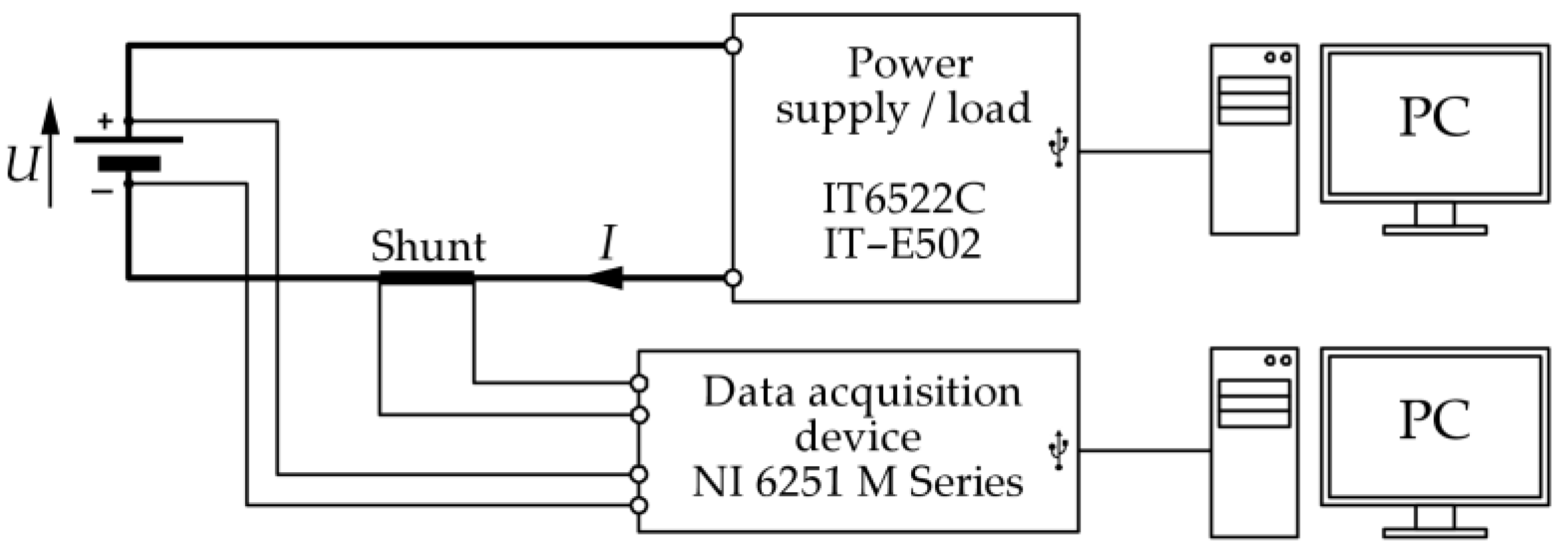
2. Materials and Methods
3. Results
3.1. Battery Cell Equivalent Circuit
3.2. Capacity and State of Charge Estimation
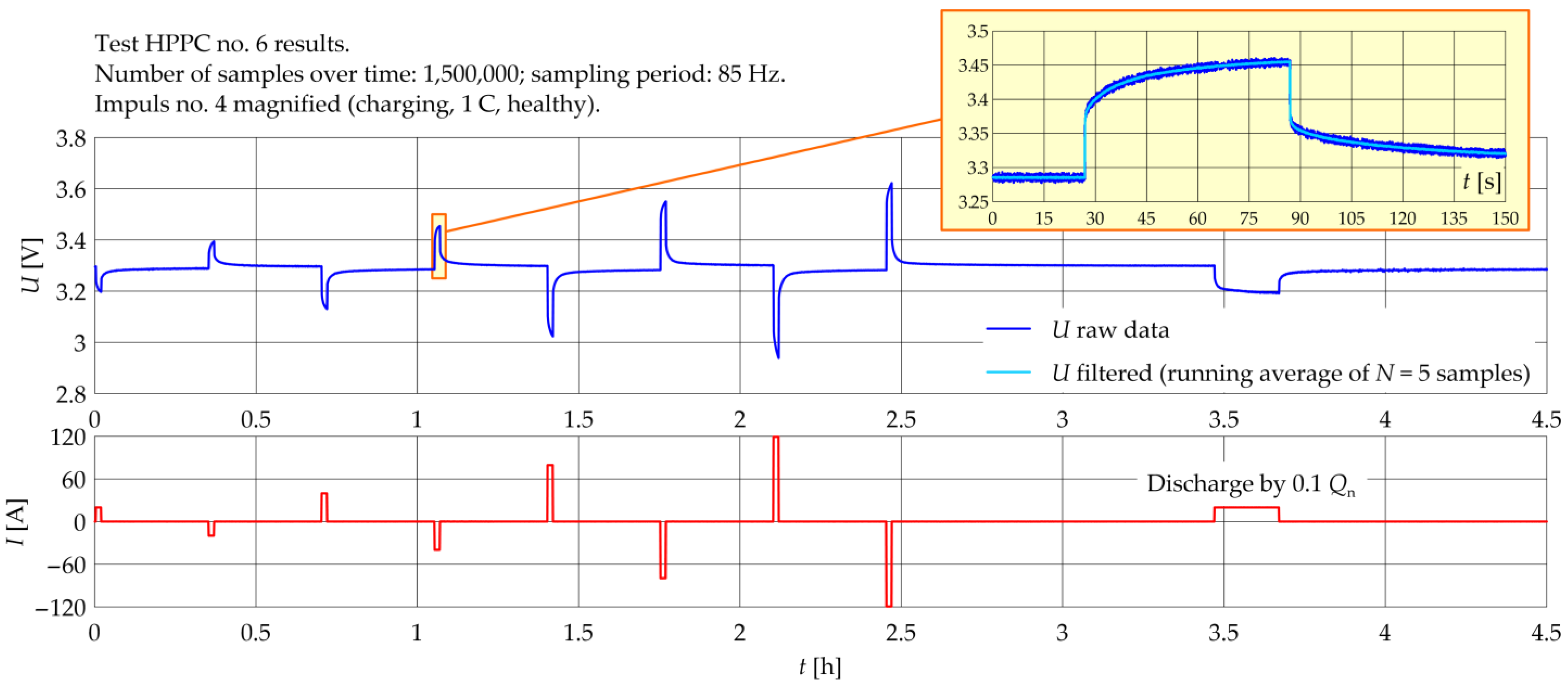
3.3. HPPC Tests
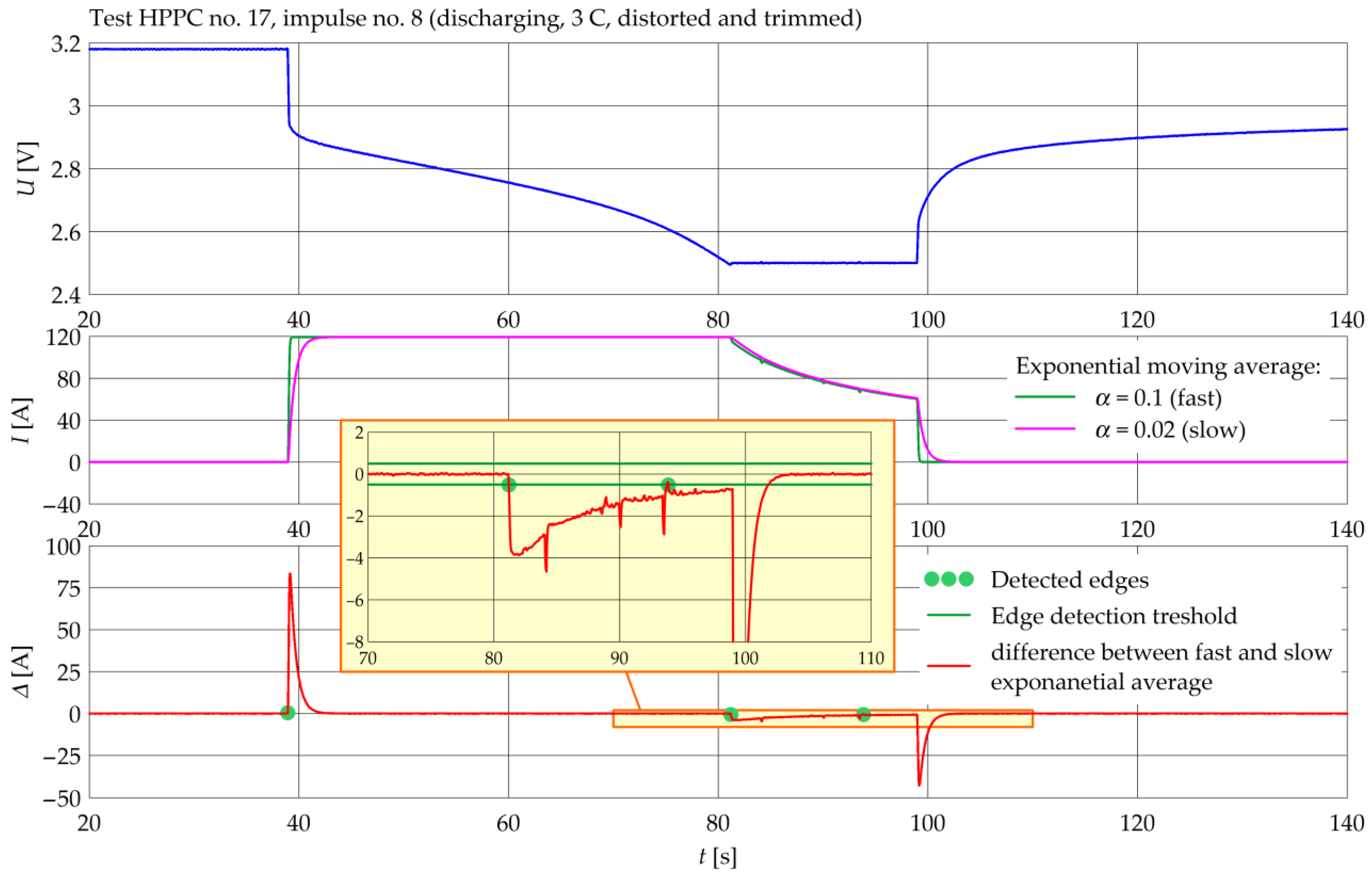
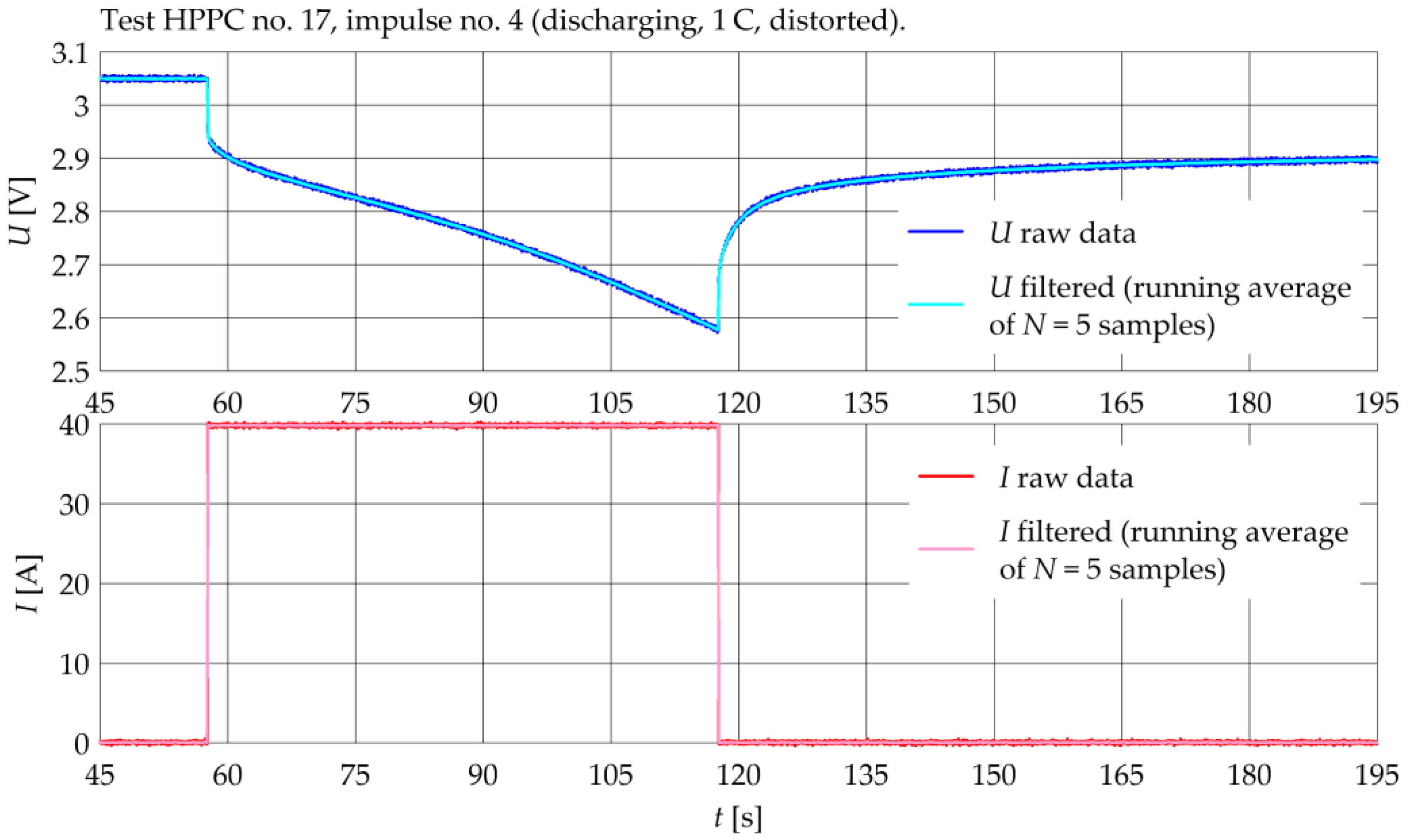
3.3.1. Filtering and Slope Detection
3.3.2. OCV vs. SOC Characteristic
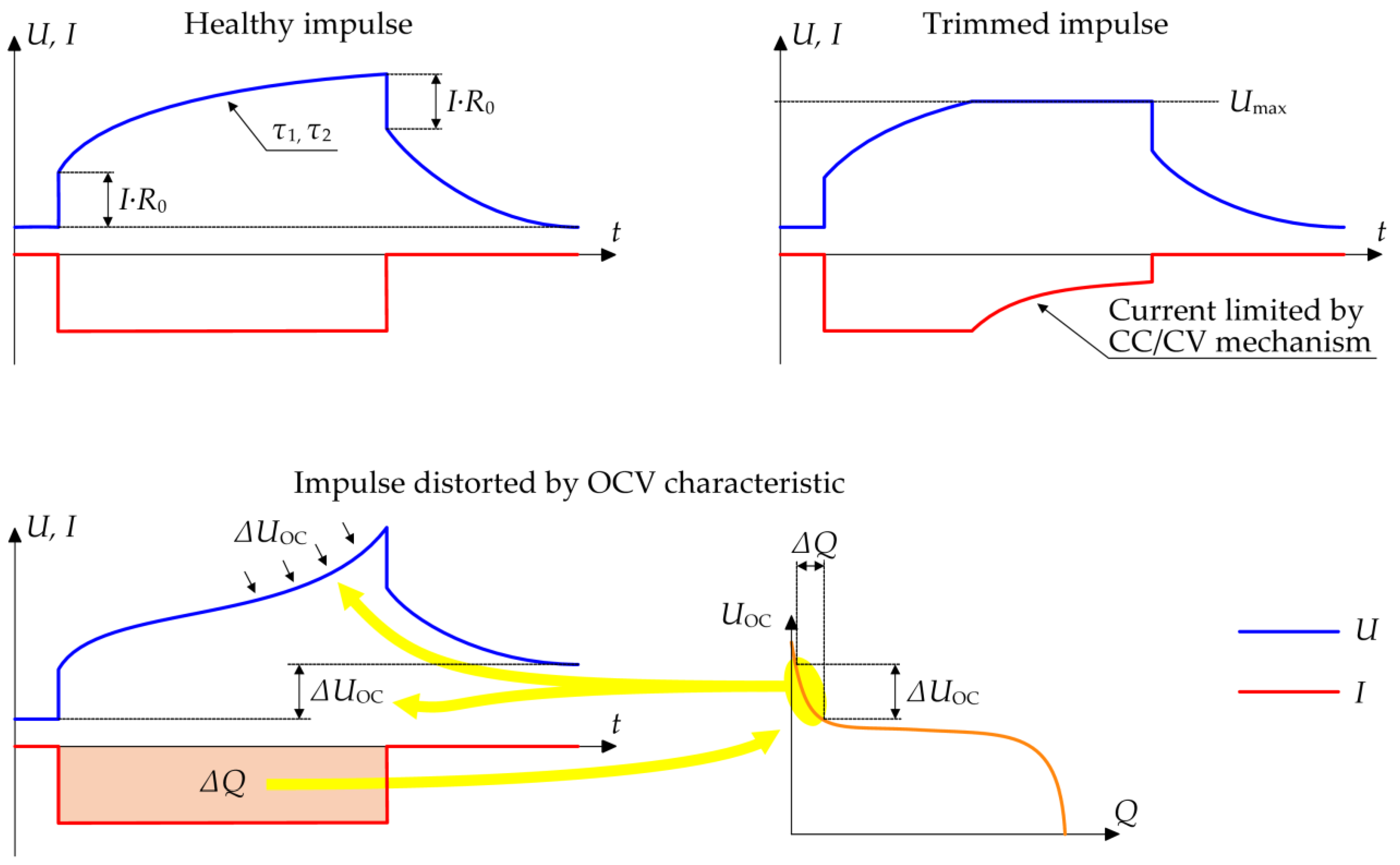
3.3.3. Impulse Evaluation and Selection
3.3.4. Impulse Waveform Approximation
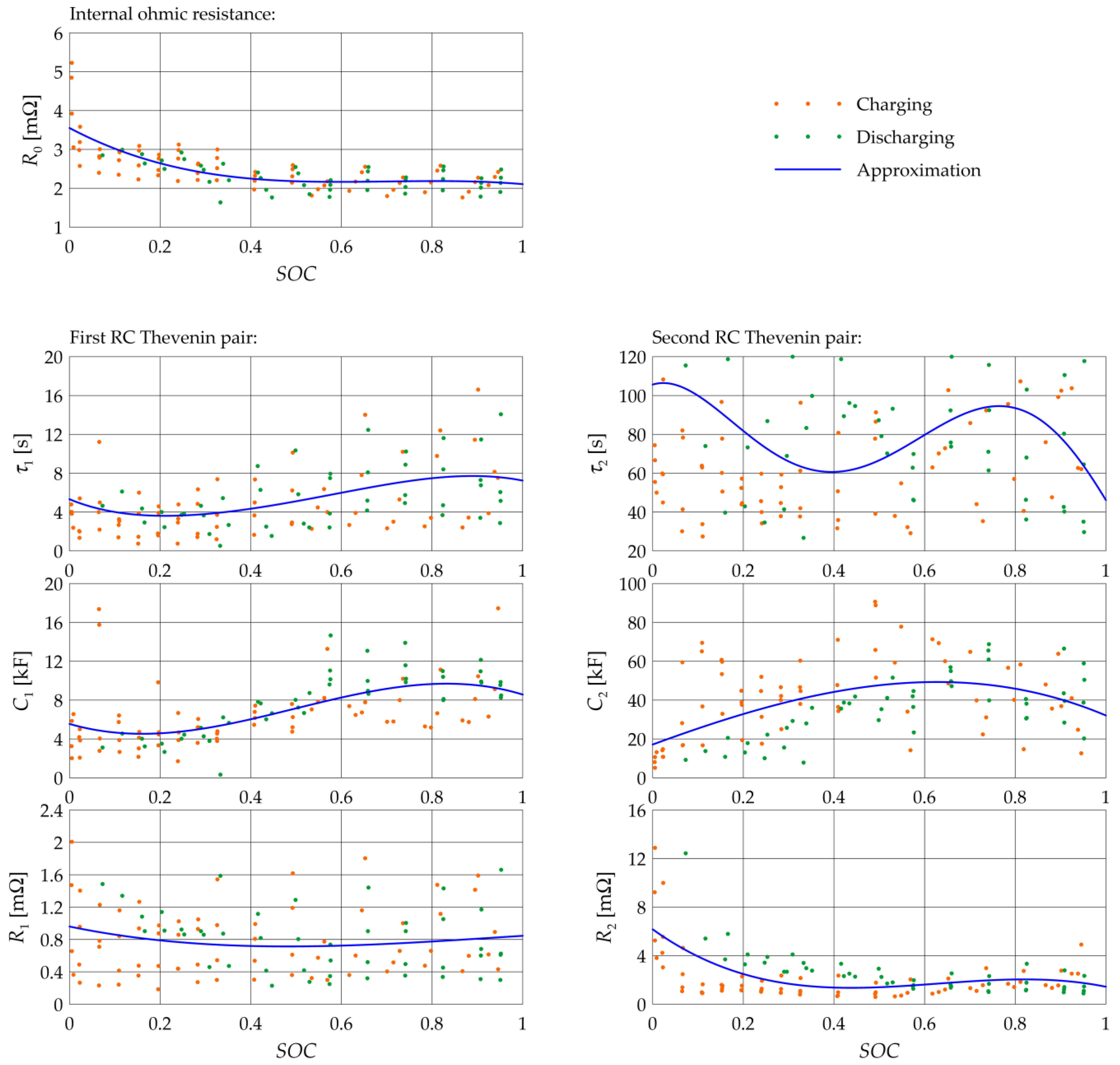
3.3.5. R and C vs. SOC Characteristics Approximation
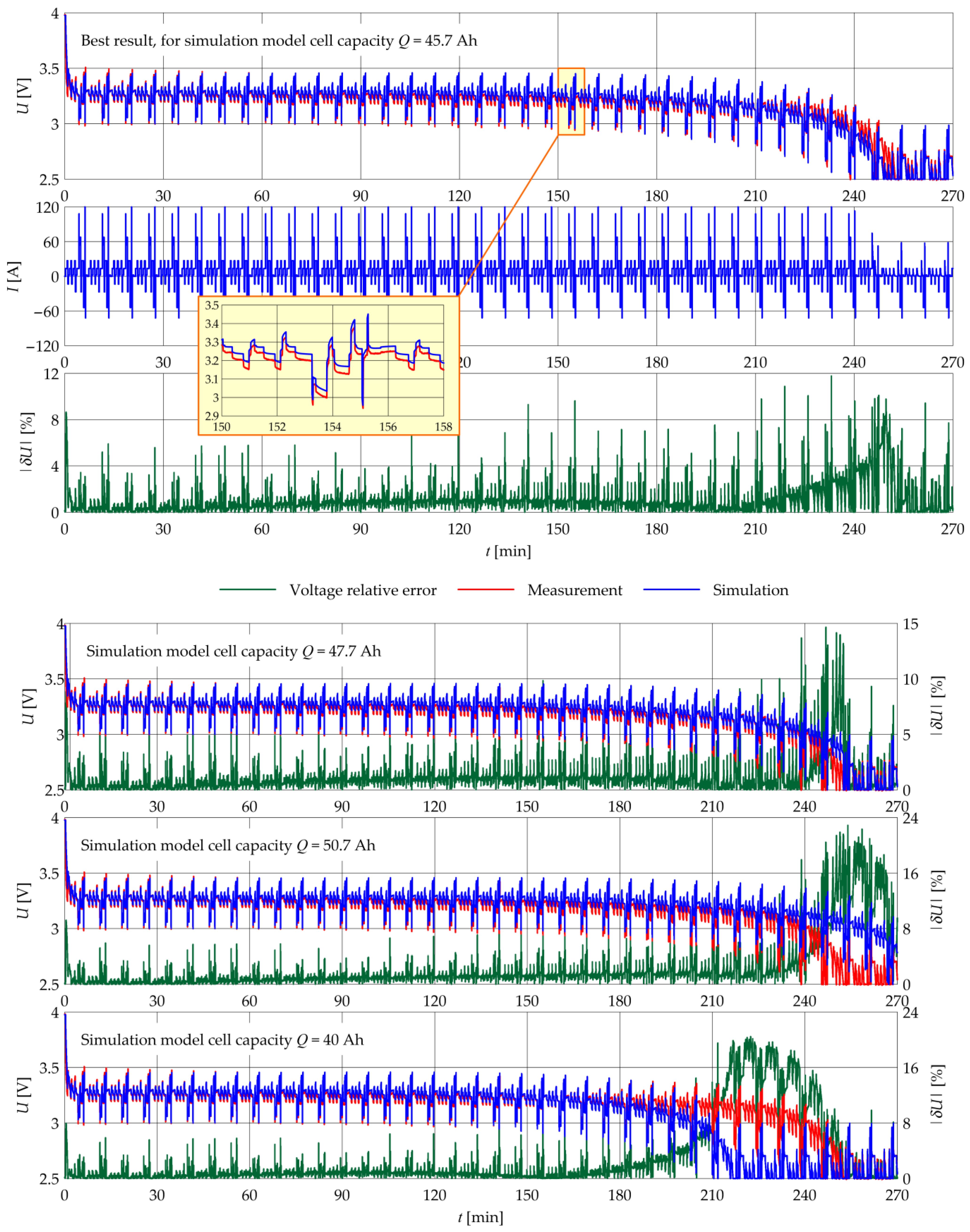
3.4. Model Verification
4. Discussion
5. Conclusions
- Among the various cell capacity values obtained as measurements, the best performance of the mathematical model was obtained for the averaged charge taken from the cell during discharge in the CC mode for different current values. Therefore, this method is recommended for determining the actual capacity of the cell.
- The OCV characteristics of the LFP cell are best approximated by the LEE function.
- Identification of the second time constant of the LFP cell is difficult, because of its large value, greater than a typical HPPC impulse duration.
- Suggestions for further research:
- It would be advisable to develop methods for automatic quality evaluation of HPPC impulses, based on the criteria given in Section 3.3.3, which would enable full automation of the HPPC test results processing.
- A method should be developed to detect the occurrence of distortion of HPPC pulses in cases where the distortion is small and does not significantly change the shape of the voltage waveform yet, but already overestimates the obtained values of time constants.
- Simulation model accuracy may be improved by better OCV characteristic approximation.
Author Contributions
Funding
Data Availability Statement
Acknowledgments
Conflicts of Interest
References
- Diampovesa, S.; Hubert, A.; Yvars, P.A. Designing physical systems through a model-based synthesis approach. Example of a Li-ion battery for electrical vehicles. Comput. Ind. 2021, 129, 103440. [Google Scholar] [CrossRef]
- Skarka, W. Model-Based Design and Optimization of Electric Vehicles. In Proceedings of the 25th ISPE International Conference on Transdisciplinary Engineering, Modena, Italy, 3–6 July 2018; Volume 7, pp. 566–575. [Google Scholar]
- Niestrój, R.; Rogala, T.; Skarka, W. An Energy Consumption Model for Designing an AGV Energy Storage System with a PEMFC Stack. Energies 2020, 13, 3435. [Google Scholar] [CrossRef]
- Mateja, K.; Skarka, W.; Peciak, M.; Niestrój, R.; Gude, M. Energy Autonomy Simulation Model of Solar Powered UAV. Energies 2023, 16, 479. [Google Scholar] [CrossRef]
- Peciak, M.; Skarka, W.; Mateja, K.; Gude, M. Impact Analysis of Solar Cells on Vertical Take-Off and Landing (VTOL) Fixed-Wing UAV. Aerospace 2023, 10, 247. [Google Scholar] [CrossRef]
- Giannelos, S.; Borozan, S.; Aunedi, M.; Zhang, X.; Ameli, H.; Pudjianto, D.; Konstantelos, I.; Strbac, G. Modelling Smart Grid Technologies in Optimisation Problems for Electricity Grids. Energies 2023, 16, 5088. [Google Scholar] [CrossRef]
- Giannelos, S.; Djapic, P.; Pudjianto, D.; Strbac, G. Quantification of the Energy Storage Contribution to Security of Supply through the F-Factor Methodology. Energies 2020, 13, 826. [Google Scholar] [CrossRef]
- Raventós, O.; Bartels, J. Evaluation of Temporal Complexity Reduction Techniques Applied to Storage Expansion Planning in Power System Models. Energies 2020, 13, 988. [Google Scholar] [CrossRef]
- Tang, Z.; Song, A.; Wang, S.; Cheng, J.; Tao, C. Numerical Analysis of Heat Transfer Mechanism of Thermal Runaway Propagation for Cylindrical Lithium-ion Cells in Battery Module. Energies 2020, 13, 1010. [Google Scholar] [CrossRef]
- Li, N.; Zhang, H.; Zhang, X.; Ma, X.; Guo, S. How to Select the Optimal Electrochemical Energy Storage Planning Program? A Hybrid MCDM Method. Energies 2020, 13, 931. [Google Scholar] [CrossRef]
- Davis, K.; Hayes, J.G. Comparison of Lithium-Ion Battery Pack Models Based on Test Data from Idaho and Argonne National Laboratories. In Proceedings of the IEEE Energy Conversion Congress and Exposition (ECCE), Detroit, MI, USA, 11–15 October 2020; pp. 5626–5632. [Google Scholar] [CrossRef]
- Rahmoun, A.; Biechl, H. Modelling of li-ion batteries using equivalent circuit diagrams. Electr. Rev. 2012, 2, 152–156. [Google Scholar]
- Tremblay, O.; Dessaint, L.; Dekkiche, A. A Generic Battery Model for the Dynamic Simulation of Hybrid Electric Vehicles. In Proceedings of the IEEE Vehicle Power and Propulsion Conference, Arlington, TX, USA, 9–12 September 2007; pp. 274–279. [Google Scholar] [CrossRef]
- Cipin, R.; Toman, M.; Prochazka, P.; Pazdera, I. Identification of Li-ion Battery Model Parameters. In Proceedings of the International Conference on Electrical Drives & Power Electronics (EDPE), The High Tatras, Slovakia, 24–26 September 2019; pp. 225–229. [Google Scholar] [CrossRef]
- Chen, S.X.; Tseng, K.J.; Choi, S.S. Modeling of Lithium-Ion Battery for Energy Storage System Simulation. In Proceedings of the Asia-Pacific Power and Energy Engineering Conference, Wuhan, China, 28–30 March 2009; pp. 1–4. [Google Scholar] [CrossRef]
- Huang, K.; Wang, Y.; Feng, J. Research on equivalent circuit Model of Lithium-ion battery for electric vehicles. In Proceedings of the 3rd World Conference on Mechanical Engineering and Intelligent Manufacturing (WCMEIM), Shanghai, China, 4–6 December 2020; pp. 492–496. [Google Scholar] [CrossRef]
- He, H.; Xiong, R.; Fan, J. Evaluation of Lithium-Ion Battery Equivalent Circuit Models for State of Charge Estimation by an Experimental Approach. Energies 2011, 4, 582–598. [Google Scholar] [CrossRef]
- Sibi Krishnan, K.; Pathiyil, P.; Sunitha, R. Generic Battery model covering self-discharge and internal resistance variation. In Proceedings of the IEEE 6th International Conference on Power Systems (ICPS), New Delhi, India, 4–6 March 2016; pp. 1–5. [Google Scholar] [CrossRef]
- Wu, W.; Qin, L.; Wu, G. State of power estimation of power lithium-ion battery based on an equivalent circuit model. J. Energy Storage 2022, 51, 104538. [Google Scholar] [CrossRef]
- Khattak, A.A.; Khan, A.N.; Safdar, M.; Basit, A.; Zaffar, N.A. A Hybrid Electric Circuit Battery Model Capturing Dynamic Battery Characteristics. In Proceedings of the IEEE Kansas Power and Energy Conference (KPEC), Manhattan, KS, USA, 13–14 July 2020; pp. 1–6. [Google Scholar] [CrossRef]
- Mueller, K.; Schwiederik, E.; Tittel, D. Analysis of parameter identification methods for electrical Li-Ion battery modelling. In Proceedings of the World Electric Vehicle Symposium and Exhibition (EVS27), Barcelona, Spain, 17–20 November 2013; pp. 1–9. [Google Scholar] [CrossRef]
- Meng, J.; Yue, M.; Diallo, D. Nonlinear extension of battery constrained predictive charging control with transmission of Jacobian matrix. Int. J. Electr. Power Energy Syst. 2023, 146, 108762. [Google Scholar] [CrossRef]
- Komal, S.; Kamyar, M.; Zunaib, A. Online reduced complexity parameter estimation technique for equivalent circuit model of lithium-ion battery. Electr. Power Syst. Res. 2020, 185, 106356. [Google Scholar] [CrossRef]
- Maletić, F.; Deur, J. Analysis of ECM-based Li-Ion Battery State and Parameter Estimation Accuracy in the Presence of OCV and Polarization Dynamics Modeling Errors. In Proceedings of the IEEE 29th International Symposium on Industrial Electronics (ISIE), Delft, The Netherlands, 17–19 June 2020; pp. 1318–1324. [Google Scholar] [CrossRef]
- Simin, P.; Gang, S.; Yunfeng, C.; Xu, C. Control of different-rating battery energy storage system interface to a microgrid. Przegląd Elektrotechniczny (Electr. Rev.) 2011, 87, 256–262. [Google Scholar]
- Meng., J.; Boukhnifer, M.; Diallo, D. Lihtium-ion battery monitoring and observability analysis with extended equivalent circuit model. In Proceedings of the IEEE Mediterranean Conference on Control and Automation (MED), Saint-Raphaël, France, 15–18 September 2020; pp. 764–769. [Google Scholar]
- Westerhoff, U.; Kurbach, K.; Lienesch, F.; Kurrat, M. Analysis of lithium-ion battery models based on electrochemical impedance spectroscopy. Energy Technol. 2016, 4, 1620–1630. [Google Scholar] [CrossRef]
- Stroe, D.I.; Swierczynski, M.; Stroe, A.I.; Knudsen Kær, S. Generalized Characterization Methodology for Performance Modelling of Lithium-Ion Batteries. Batteries 2016, 2, 37. [Google Scholar] [CrossRef]
- Cordoba-Arenas, A.; Onori, S.; Rizzoni, G.A. Control-oriented lithium-ion battery pack model for plug-in hybrid electric vehicle cycle-life studies and systems design with consideration of health management. J. Power Sources 2015, 279, 791–808. [Google Scholar] [CrossRef]
- Liaw, B.Y.; Nagasubramanian, G.; Jungst, R.G.; Doughty, D.H. Modeling of lithium ion cells—A simple equivalent-circuit model approach. Solid State Ion. 2004, 175, 835–839. [Google Scholar] [CrossRef]
- Huria, T.; Ceraolo, M.; Gazzarri, J.; Jackey, R. High fidelity electrical model with thermal dependence for characterization and simulation of high power lithium battery cells. In Proceedings of the IEEE International Electric Vehicle Conference, Greenville, SC, USA, 4–8 March 2012; pp. 1–8. [Google Scholar] [CrossRef]
- Sockeel, N.; Shahverdi, M.; Mazzola, M.; Meadows, W. High-Fidelity Battery Model for Model Predictive Control Implemented into a Plug-In Hybrid Electric Vehicle. Batteries 2017, 3, 13. [Google Scholar] [CrossRef]
- Li, K.; Soong, B.H.; Tseng, K.J. A high-fidelity hybrid lithium-ion battery model for SOE and runtime prediction. In Proceedings of the IEEE Applied Power Electronics Conference and Exposition (APEC), Tampa, FL, USA, 26–30 March 2017; pp. 2374–2381. [Google Scholar] [CrossRef]
- Hemi, H.; M’Sirdi, N.K.; Naamane, A.; Ikken, B. Open Circuit Voltage of a Lithium ion Battery Model Adjusted by Data Fitting. In Proceedings of the 6th International Renewable and Sustainable Energy Conference (IRSEC), Rabat, Morocco, 5–8 December 2018; pp. 1–5. [Google Scholar]
- Zhang, Q.; Shang, Y.; Li, Y.; Cui, N.; Duan, B.; Zhang, C. A novel fractional variable-order equivalent circuit model and parameter identification of electric vehicle Li-ion batteries. ISA Trans. 2020, 97, 448–457. [Google Scholar] [CrossRef]
- Baczyńska, A.; Niewiadomski, W.; Gonçalves, A.; Almeida, P.; Luís, R. Li-NMC Batteries Model Evaluation with Experimental Data for Electric Vehicle Application. Batteries 2018, 4, 11. [Google Scholar] [CrossRef]
- Somakettarin, N.; Funaki, T. Study on Factors for Accurate Open Circuit Voltage Characterizations in Mn-Type Li-Ion Batteries. Batteries 2017, 3, 8. [Google Scholar] [CrossRef]
- Gao, Y.; Ji, W.; Zhao, X. SOC Estimation of E-Cell Combining BP Neural Network and EKF Algorithm. Processes 2022, 10, 1721. [Google Scholar] [CrossRef]
- Rothenberger, M.J.; Docimo, D.J.; Ghanaatpishe, M.; Fathy, H.K. Genetic optimization and experimental validation of a test cycle that maximizes parameter identifiability for a Li-ion equivalent-circuit battery model. J. Energy Storage 2015, 4, 156–166. [Google Scholar] [CrossRef]
- Nemes, R.; Ciornei, S.; Ruba, M.; Hedesiu, H.; Martis, C. Modeling and simulation of first-order Li-Ion battery cell with experimental validation. In Proceedings of the 8th International Conference on Modern Power Systems (MPS), Cluj-Napoca, Romania, 21–23 May 2019; pp. 1–6. [Google Scholar] [CrossRef]
- Nemes, R.O.; Ciornei, S.M.; Ruba, M.; Martis, C. Parameters identification using experimental measurements for equivalent circuit Lithium-Ion cell models. In Proceedings of the 11th International Symposium on Advanced Topics in Electrical Engineering (ATEE), Bucharest, Romania, 28–30 March 2019; pp. 1–6. [Google Scholar] [CrossRef]
- Hua, X.; Zhang, C.; Offer, G. Finding a better fit for lithium ion batteries: A simple, novel, load dependent, modified equivalent circuit model and parameterization method. J. Power Sources 2021, 484, 229117. [Google Scholar] [CrossRef]
- Li, Z.; Shi, X.; Shi, M.; Wei, C.; Di, F.; Sun, H. Investigation on the Impact of the HPPC Profile on the Battery ECM Parameters’ Offline Identification. In Proceedings of the Asia Energy and Electrical Engineering Symposium (AEEES), Chengdu, China, 28–31 May 2020; pp. 753–757. [Google Scholar] [CrossRef]
- Haghjoo, Y.; Khaburi, D.A. Modeling, simulation, and parameters identification of a lithium-ion battery used in electric vehicles. In Proceedings of the 9th Iranian Conference on Renewable Energy & Distributed Generation (ICREDG), Mashhad, Iran, 23–24 February 2022; pp. 1–7. [Google Scholar] [CrossRef]
- Tran, M.K.; Mathew, M.; Janhunen, S.; Panchal, S.; Raahemifar, K.; Fraser, R.; Fowler, M. A comprehensive equivalent circuit model for lithium-ion batteries, incorporating the effects of state of health, state of charge, and temperature on model parameters. J. Energy Storage 2021, 43, 103252. [Google Scholar] [CrossRef]
- Deng, S.D.; Liu, S.Y.; Wang, L.; Xia, L.L.; Chen, L. An improved second-order electrical equivalent modeling method for the online high power Li-ion battery state of charge estimation. In Proceedings of the IEEE 12th Energy Conversion Congress & Exposition—Asia (ECCE-Asia), Singapore, 24–27 May 2021; pp. 1725–1729. [Google Scholar] [CrossRef]
- Parthasarathy, C.; Laaksonen, H.; Halagi, P. Characterisation and Modelling Lithium Titanate Oxide Battery Cell by Equivalent Circuit Modelling Technique. In Proceedings of the IEEE PES Innovative Smart Grid Technologies—Asia (ISGT Asia), Brisbane, Australia, 5–8 December 2021; pp. 1–5. [Google Scholar] [CrossRef]
- Navas, S.J.; Cabello González, G.M.; Pino, F.J.; Guerra, J.J. Modelling Li-ion batteries using equivalent circuits for renewable energy applications. Energy Rep. 2023, 9, 4456–4465. [Google Scholar] [CrossRef]
- Wang, J.; Jia, Y.; Yang, N.; Lu, Y.; Shi, M.; Ren, X.; Lu, D. Precise equivalent circuit model for Li-ion battery by experimental improvement and parameter optimization. J. Energy Storage 2022, 52, 104980. [Google Scholar] [CrossRef]
- Sörés, M.A.; Hartmann, B. Overview of possible methods of determining self-discharge. In Proceedings of the IEEE International Conference on Environment and Electrical Engineering and IEEE Industrial and Commercial Power Systems Europe (EEEIC/I&CPS Europe), Madrid, Spain, 9–12 June 2020; pp. 1–5. [Google Scholar] [CrossRef]
- Tang, A.; Gong, P.; Li, J.; Zhang, K.; Zhou, Y.; Zhang, Z. A State-of-Charge Estimation Method Based on Multi-Algorithm Fusion. World Electr. Veh. J. 2022, 13, 70. [Google Scholar] [CrossRef]
- Jarrraya, I.; Degaa, L.; Rizoug, N.; Chabchoub, M.H.; Trabelsi, H. Comparison study between hybrid Nelder-Mead particle swarm optimization and open circuit voltage—Recursive least square for the battery parameters estimation. J. Energy Storage 2022, 50, 104424. [Google Scholar] [CrossRef]
- Castanho, D.; Guerreiro, M.; Silva, L.; Eckert, J.; Antonini Alves, T.; Tadano, Y.d.S.; Stevan, S.L., Jr.; Siqueira, H.V.; Corrêa, F.C. Method for SoC Estimation in Lithium-Ion Batteries Based on Multiple Linear Regression and Particle Swarm Optimization. Energies 2022, 15, 6881. [Google Scholar] [CrossRef]
- Pizarro-Carmona, V.; Castano-Solís, S.; Cortés-Carmona, M.; Fraile-Ardanuy, J.; Jimenez-Bermejo, G. GA-based approach to optimize an equivalent electric circuit model of a Li-ion battery-pack. Expert Syst. Appl. 2021, 172, 114647. [Google Scholar] [CrossRef]
- Huang, Y.; Li, Y.; Jiang, L.; Qiao, X.; Cao, Y.; Yu, J. Research on Fitting Strategy in HPPC Test for Li-ion battery. In Proceedings of the IEEE Sustainable Power and Energy Conference (iSPEC), Beijing, China, 21–23 November 2019; pp. 1776–1780. [Google Scholar] [CrossRef]
- Wang, C.; Xu, M.; Zhang, Q.; Feng, J.; Jiang, R.; Wei, Y.; Liu, Y. Parameters identification of Thevenin model for lithium-ion batteries using self-adaptive Particle Swarm Optimization Differential Evolution algorithm to estimate state of charge. J. Energy Storage 2021, 44, 103244. [Google Scholar] [CrossRef]
- Hamida, M.A.; El-Sehiemy, R.A.; Ginidi, A.R.; Elattar, E.; Shaheen, A.M. Parameter identification and state of charge estimation of Li-Ion batteries used in electric vehicles using artificial hummingbird optimizer. J. Energy Storage 2022, 51, 104535. [Google Scholar] [CrossRef]
- Szewczyk, P.; Łebkowski, A. Comparative Studies on Batteries for the Electrochemical Energy Storage in the Delivery Vehicle. Energies 2022, 15, 9613. [Google Scholar] [CrossRef]
- Łebkowski, Ł. Temperature, Overcharge and Short-Circuit Studies of Batteries used in Electric Vehicles. Prz. Elektrotechniczny 2017, 93, 67–73. [Google Scholar] [CrossRef]
- Ohneseit, S.; Finster, P.; Floras, C.; Lubenau, N.; Uhlmann, N.; Seifert, H.J.; Ziebert, C. Thermal and Mechanical Safety Assessment of Type 21700 Lithium-Ion Batteries with NMC, NCA and LFP Cathodes–Investigation of Cell Abuse by Means of Accelerating Rate Calorimetry (ARC). Batteries 2023, 9, 237. [Google Scholar] [CrossRef]
- Kiemel, S.; Glöser-Chahoud, S.; Waltersmann, L.; Schutzbach, M.; Sauer, A.; Miehe, R. Assessing the Application-Specific Substitutability of Lithium-Ion Battery Cathode Chemistries Based on Material Criticality, Performance, and Price. Resources 2021, 10, 87. [Google Scholar] [CrossRef]
- Forte, F.; Pietrantonio, M.; Pucciarmati, S.; Puzone, M.; Fontana, D. Lithium Iron Phosphate Batteries Recycling: An Assessment of Current Status. Crit. Rev. Environ. Sci. Technol. 2021, 51, 2232–2259. [Google Scholar]
- Białoń, T.; Niestrój, R.; Korski, W. PSO-Based Identification of the Li-Ion Battery Cell Parameters. Energies 2023, 16, 3995. [Google Scholar] [CrossRef]
- Belt, J.R. Battery Test Manual for Plug-In Hybrid Electric Vehicles, 2nd ed.; U.S. Department of Energy Vehicle Technologies Program: Idaho Falls, ID, USA, 2010. [Google Scholar] [CrossRef]
- Yang, Z.; Wang, X. An improved parameter identification method considering multi-timescale characteristics of lithium-ion batteries. J. Energy Storage 2023, 59, 106462. [Google Scholar] [CrossRef]
- Karimi, D.; Behi, H.; Van Mierlo, J.; Berecibar, M. Equivalent Circuit Model for High-Power Lithium-Ion Batteries under High Current Rates, Wide Temperature Range, and Various State of Charges. Batteries 2023, 9, 101. [Google Scholar] [CrossRef]
- Guenther, C.; Barillas, J.K.; Stumpp, S.; Danzer, M.A. A dynamic battery model for simulation of battery-to-grid applications. In Proceedings of the 3rd IEEE PES Innovative Smart Grid Technologies Europe (ISGT Europe), Berlin, Germany, 14–17 October 2012; pp. 1–7. [Google Scholar] [CrossRef]
- Shi, J.; Guo, H.; Chen, D. Parameter identification method for lithium-ion batteries based on recursive least square with sliding window difference forgetting factor. J. Energy Storage 2021, 44, 103485. [Google Scholar] [CrossRef]
- Tran, M.-K.; DaCosta, A.; Mevawalla, A.; Panchal, S.; Fowler, M. Comparative Study of Equivalent Circuit Models Performance in Four Common Lithium-Ion Batteries: LFP, NMC, LMO, NCA. Batteries 2021, 7, 51. [Google Scholar] [CrossRef]
- Feng, D.; Huang, J.; Jin, P.; Chen, H.; Wang, A.; Zheng, M. Parameter Identification and Dynamic Simulation of Lithium-Ion Power Battery Based on DP Model. In Proceedings of the 14th IEEE Conference on Industrial Electronics and Applications (ICIEA), Xi’an, China, 19–21 June 2019; pp. 1275–1279. [Google Scholar] [CrossRef]
- Einhorn, M.; Conte, V.F.; Kral, C.; Fleig, J.; Permann, R. Parameterization of an electrical battery model for dynamic system simulation in electric vehicles. In Proceedings of the IEEE Vehicle Power and Propulsion Conference, Lille, France, 1–3 September 2010; pp. 1–7. [Google Scholar] [CrossRef]
- Yu, Q.; Wan, C.; Li, J.; E, L.; Zhang, X.; Huang, Y.; Liu, T. An Open Circuit Voltage Model Fusion Method for State of Charge Estimation of Lithium-Ion Batteries. Energies 2021, 14, 1797. [Google Scholar] [CrossRef]
- Gao, L.; Liu, S.; Dougal, R.A. Dynamic lithium-ion battery model for system simulation. IEEE Trans. Compon. Packag. Technol. 2002, 25, 495–505. [Google Scholar] [CrossRef]
- Wen, F.; Duan, B.; Zhang, C.; Zhu, R.; Shang, Y.; Zhang, J. High-Accuracy Parameter Identification Method for Equivalent-Circuit Models of Lithium-Ion Batteries Based on the Stochastic Theory Response Reconstruction. Electronics 2019, 8, 834. [Google Scholar] [CrossRef]
- Baccouche, I.; Jemmali, S.; Manai, B.; Omar, N.; Amara, N.E.B. Improved OCV Model of a Li-Ion NMC Battery for Online SOC Estimation Using the Extended Kalman Filter. Energies 2017, 10, 764. [Google Scholar] [CrossRef]
- Pillai, P.; Sundaresan, S.; Kumar, P.; Pattipati, K.R.; Balasingam, B. Open-Circuit Voltage Models for Battery Management Systems: A Review. Energies 2022, 15, 6803. [Google Scholar] [CrossRef]
- Shaheen, A.M.; Hamida, M.A.; El-Sehiemy, R.A.; Elattar, E.E. Optimal parameter identification of linear and non-linear models for Li-Ion Battery Cells. Energy Rep. 2021, 7, 7170–7185. [Google Scholar] [CrossRef]
- Plett, G.L. High-performance battery-pack power estimation using a dynamic cell model. IEEE Trans. Veh. Technol. 2004, 53, 1586–1593. [Google Scholar] [CrossRef]
- Marušić, D.; Vašak, M. Efficient Method of Identifying a Li-Ion Battery Model for an Electric Vehicle. In Proceedings of the IEEE 20th International Power Electronics and Motion Control Conference (PEMC), Brasov, Romania, 25–28 September 2022; pp. 421–426. [Google Scholar] [CrossRef]


| Parameter | Value |
|---|---|
| Capacity Qn | 40 Ah |
| Energy density | 82.5 Wh/kg |
| Voltage (min./nominal/max.) | 2.5/3.3/4.0 |
| Current (typical/max. discharge) | 20 A (0.5C 1)/400 A (10C 1) |
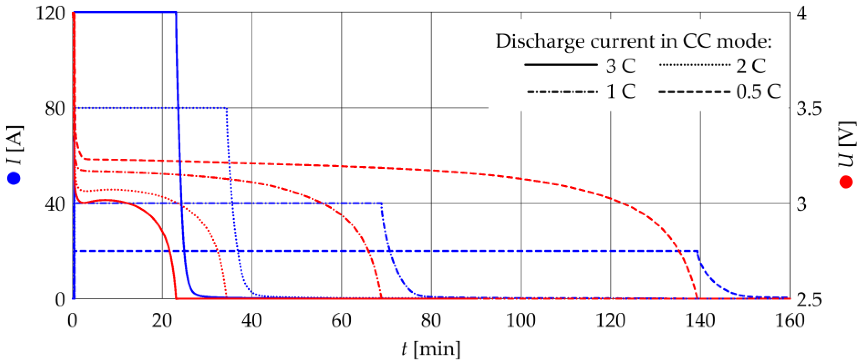
| Relative Discharge Current | Total Discharge Q [Ah] | Discharge in CC Mode QCC [Ah] | Discharge in CV Mode QCV [Ah] |
|---|---|---|---|
| 0.5C | 47.71 | 46.30 | 1.407 |
| 1C | 47.71 | 45.78 | 1.934 |
| 2C | 47.70 | 45.21 | 2.495 |
| 3C | 47.62 | 45.41 | 2.212 |
| HPPC Test No. | Impulse No., Type and Relative Current Value | ΔQ [Ah] | ΔQ/Qn [%] | Q [Ah] | |||||||
|---|---|---|---|---|---|---|---|---|---|---|---|
| 1 0.5 C | 2 0.5 C | 3 1 C | 4 1 C | 5 2 C | 6 2 C | 7 3 C | 8 3 C | ||||
| 1 | (−) | (+) | (−) | (+) | (−) | (+) | (−) | (+) | 2.41 | 6.03 | 2.41 |
| 2 | (−) | (+) | (−) | (+) | (−) | (+) | (−) | (+) | 2.21 | 5.53 | 4.63 |
| 3 | (−) | (+) | (−) | (+) | (−) | (+) | (−) | (+) | 4.21 | 10.53 | 8.84 |
| 4 | (−) | (+) | (−) | (+) | (−) | (+) | (−) | (+) | 4.21 | 10.53 | 13.05 |
| 5 | (−) | (+) | (−) | (+) | (−) | (+) | (−) | (+) | 4.22 | 10.54 | 17.27 |
| 6 | (−) | (+) | (−) | (+) | (−) | (+) | (−) | (+) | 4.23 | 10.57 | 21.50 |
| 7 | (−) | (+) | (−) | (+) | (−) | (+) | (−) | (+) | 4.22 | 10.56 | 25.72 |
| 8 | (+) | (−) | (+) | (−) | (+) | (−) | (+) | (−) | 4.21 | 10.54 | 29.93 |
| 9 | (+) | (−) | (+) | (−) | (+) | (−) | (+) | (−) | 4.22 | 10.55 | 34.16 |
| 10 | (+) | (−) | (+) | (−) | (+) | (−) | (+) | (−) | 2.16 | 5.40 | 36.31 |
| 11 | (+) | (−) | (+) | (−) | (+) | (−) | (+) | (−) | 2.18 | 5.45 | 38.49 |
| 12 | (+) | (−) | (+) | (−) | (+) | (−) | (+) | (−) | 2.20 | 5.51 | 40.70 |
| 13 | (+) | (−) | (+) | (−) | (+) | (−) | (+) | (−) | 2.21 | 5.52 | 42.90 |
| 14 | (+) | (−) | (+) | (−) | (+) | (−) | (+) | (−) | 2.22 | 5.54 | 45.12 |
| 15 | (+) | (−) | (+) | (−) | (+) | (−) | (+) | (−) | 2.20 | 5.49 | 47.32 |
| 16 | (+) | (−) | (+) | (−) | (+) | (−) | (+) | (−) | 2.22 | 5.55 | 49.54 |
| 17 | (+) | (−) | (+) | (−) | (+) | (−) | (+) | (−) | 0.92 | 2.31 | 50.46 |
| 18 | (+) | (−) | (+) | (−) | (+) | (−) | (+) | (−) | 0.25 | 0.62 | 50.71 |
| a | b | c | d | |
|---|---|---|---|---|
| R0 | 3.551 × 10⁻³ | −6.172 × 10⁻³ | 8.993 × 10⁻³ | −4.267 × 10⁻³ |
| R1 | 9.601 × 10⁻⁴ | −1.154 × 10⁻³ | 1.611 × 10⁻³ | −5.716 × 10⁻⁴ |
| R2 | 6.169 × 10⁻³ | −2.678 × 10⁻² | 4.690 × 10⁻² | −2.485 × 10⁻² |
| C1 | 5549 | −1.359 × 10⁴ | 5.058 × 10⁴ | −3.397 × 10⁴ |
| C2 | 1.712 × 10⁴ | 8.510 × 10⁴ | −2.850 × 10⁴ | −4.243 × 10⁴ |
| Voltage RMS Error | Cell Capacity Q [Ah] | Comment |
|---|---|---|
| 0.0432 | 45.7 | Average for discharge characteristics, CC mode only |
| 0.0487 | 47.7 | Average for discharge characteristics, CC + CV |
| 0.120 | 50.7 | HPPC tests total discharge |
| 0.167 | 40.0 | Qn—nominal cell capacity |
| Cell Capacity Q [Ah] | Average Error |δU| [%] | Average Error for t from 5 min to 180 min |δU| [%] | Peak Error |δU| [%] | Peak Error for t from 5 min to 180 min |δU| [%] |
|---|---|---|---|---|
| 45.7 | 0.977 | 0.751 | 14.9 | 9.62 |
| 47.7 | 1.07 | 0.805 | 14.6 | 9.83 |
| 50.7 | 2.44 | 0.873 | 22.9 | 10.1 |
| 40 | 2.73 | 0.579 | 20.4 | 9.04 |
Disclaimer/Publisher’s Note: The statements, opinions and data contained in all publications are solely those of the individual author(s) and contributor(s) and not of MDPI and/or the editor(s). MDPI and/or the editor(s) disclaim responsibility for any injury to people or property resulting from any ideas, methods, instructions or products referred to in the content. |
© 2023 by the authors. Licensee MDPI, Basel, Switzerland. This article is an open access article distributed under the terms and conditions of the Creative Commons Attribution (CC BY) license (https://creativecommons.org/licenses/by/4.0/).
Share and Cite
Białoń, T.; Niestrój, R.; Skarka, W.; Korski, W. HPPC Test Methodology Using LFP Battery Cell Identification Tests as an Example. Energies 2023, 16, 6239. https://doi.org/10.3390/en16176239
Białoń T, Niestrój R, Skarka W, Korski W. HPPC Test Methodology Using LFP Battery Cell Identification Tests as an Example. Energies. 2023; 16(17):6239. https://doi.org/10.3390/en16176239
Chicago/Turabian StyleBiałoń, Tadeusz, Roman Niestrój, Wojciech Skarka, and Wojciech Korski. 2023. "HPPC Test Methodology Using LFP Battery Cell Identification Tests as an Example" Energies 16, no. 17: 6239. https://doi.org/10.3390/en16176239
APA StyleBiałoń, T., Niestrój, R., Skarka, W., & Korski, W. (2023). HPPC Test Methodology Using LFP Battery Cell Identification Tests as an Example. Energies, 16(17), 6239. https://doi.org/10.3390/en16176239