Temperature Distribution in a Finite-Length Cylindrical Channel Filled with Biomass Transported by Electrically Heated Auger

Abstract

The heat conduction problem for a cylindrical ring reactor of finite length, filled with biomass, which is transported at a constant speed by means of a rotating screw, is considered. The screw is assumed to be mounted on a circular shaft and is inductively heated by the Joule–Lenz effect. The surfaces of the channel and the shaft are thermally insulated. At the entrance and exit of the channel, boundary conditions of the third kind are formulated. The surface of the screw is replaced by uniformly distributed point heat sources. The problem is solved using the decomposition of the investigated temperature into Fourier–Bessel series over space variables and the integral Laplace transform over time. It is shown that the temperature has a quasi-stationary character with a short-term transient process. A numerical analysis of the spatio-temporal structure of temperature and its relationship with the thermophysical, kinematic and geometric parameters of the screw and biomass was carried out. In particular, it was found that the temperature along the reactor increases almost linearly starting from 400 K. It is shown that as in the case of an infinitely long channel, the condition of space–time resonance of the temperature field is fulfilled here.

1. Introduction

Recently, the problem of improving the methods of thermochemical processing of waste and biomass has attracted increasing attention from researchers and practitioners [1,2,3,4,5,6]. At the same time, reactors in which the movement of the mixture occurs with the help of a screw with a different width of the effective surface have gained considerable popularity. The source of heat is directly an auger system (screw, spiral) heated electrically. As a result of the Joule–Lenz effect [7], the surface of the screw is heated, and due to its contact with the filler, heat is transferred to the filling medium. This makes it possible to pyrolyze waste or sterilize and roast food ingredients like vegetables, herbs, spices, etc. [8].

Both shaft and shaftless screw systems are used in industry. They are designed in such a way as to improve mechanical contact and heat exchange between solid coolants and reagents. At the same time, the rate of transfer of raw materials in the reactor is tried to be selected in such a way as to create the optimal biomass retention time and temperature conditions for the pyrolysis or sterilization to proceed. Pyrolysis requires the addition of heat not only to raise the temperature of the reactants to an appropriate level but also to stimulate the chemical reaction that occurs. As a result, the need to create such a temperature field that would provide all the necessary conditions for the pyrolysis process, as well as sterilization or pasteurization of food ingredients, becomes obvious. The study of the dynamics of heat exchange in a large reactor is necessary also for optimal control of the fast or slow pyrolysis process. In addition, it should be added that as experiments have shown [9], the temperature of pyrolysis has a great influence on the product.

Thus, one of the main problems is the mathematical analysis of the spatio-temporal characteristics of thermal conductivity in the reactor, taking into account its geometric, mechanical and thermodynamic parameters. In previous articles [10,11,12,13], we made an attempt to analytically describe the temperature field in a circular cylindrical reactor filled with a mixture of materials transported by the rotation of a screw or spiral, and it is also heated by these elements and subjected to the pyrolysis process. It was assumed that the screw is heated by an electric current due to the Joule–Lenz effect. Several types of construction of the driving and heating element of this system were considered: a screw fixed on a circular shaft [13], a screw without a shaft [10], a cylindrical helix connected to a shaft [12], and a helix without a shaft [11]. In all cases considered so far, the screw, like the reactor body, was infinitely long. It was also assumed that the surfaces of the reactor and the bearing–bearing rotating shaft were thermally insulated.

Due to the fact that reactors and screws are of finite length in real structures, there is a need to take this factor into account and solve the more complex boundary value problem of non-stationary thermal conductivity in a circular cylinder of finite length. Appropriate boundary conditions must therefore be taken into account not only at its lateral surfaces, but also at its ends, i.e., at the entrance and exit. In this paper, we consider the case of a cylindrical reactor of finite length with a screw fixed on the inner shaft. The surface of the reactor and the shaft are thermally insulated. We will assume that the convective heat transfer conditions are satisfied at the reactor inlet and outlet; i.e., we will apply boundary conditions of the third kind that is Newton’s B.C. It is necessary to find an analytical solution to this problem and to investigate the features of the spatio-temporal temperature distribution in the moving medium filling the reactor, using specific geometric, mechanical and thermodynamic parameters of the reactor, mixture and auger.

It should be noted here that in our previous studies with infinitely long reactors, the integral Fourier transform over the axial variable was applied and the exact solution of the problem was obtained. In the case of a finite-length reactor, where the boundary conditions at the inlet and outlet of the reactor must be considered, this method does not work. As shown below, the approximate method of expanding the desired solution in terms of the system of orthogonal coordinate functions, which we used here, turned out to be effective.

2. Mathematical Formulation of the Problem

Consider a heat-insulated circular cylindrical channel of radius R₁ and finite length L filled with a mixture of biomass. The biomass material moves in the axial direction with a velocity v₀ due to the rotation of the screw attached to the heat-insulated shaft of radius R₂ (R₁ > R₂) which is rotated with an angular velocity ω. The heating of the mixed biomass material occurs due to heat transfer from a screw, which in turn is heated due to the Joule–Lenz thermoelectric effect by an electric current I evenly distributed over the surface of the screw. Due to the interaction of biomass particles during its movement and heating, complex thermochemical processes take place in the reactor. The object of research of this article is the spatio-temporal distribution of temperature in the reactor, since temperature is the main driving force of the biomass pyrolysis reaction.

For a mathematical description of the temperature field in a ring channel filled with a continuum of moving biomass as pseudo-liquid, it is necessary to solve the differential equation of non-stationary thermal conductivity [14]

$$\begin{array}{l}{c}_p\rho \left(\frac{\partial T}{\partial \tau }+v_0\frac{\partial T}{\partial z}\right)=\lambda \left[\frac{1}{r}\frac{\partial }{\partial r}\left(r\frac{\partial T}{\partial r}\right)+\frac{1}{r^2}\frac{{\partial }^{2}T}{\partial {\theta }^2}+\frac{{\partial }^{2}T}{\partial z^2}\right]+q \left(r, \theta ,z, \tau \right)\\ \left(R_2<r<R_1, 0<\theta <2\pi , 0<z<L , \tau >0\right)\end{array}$$

(1)

with the initial condition

$${T|}_{\tau =0}=T_0,$$

(2)

and the boundary conditions of thermal insulation on the surface of the channel

$${\frac{\partial T}{\partial r}|}_{r=R_1}=0$$

(3)

and on the surface of the screw shaft

$${\frac{\partial T}{\partial r}|}_{r=R_2}=0,$$

(4)

and also with the boundary conditions of linear heat transfer at the end surfaces of the channel

$${\lambda \frac{\partial T}{\partial z}|}_{z=0}=-h\left(T_{in}-{T|}_{z=0}\right),$$

(5)

$${\lambda \frac{\partial T}{\partial z}|}_{z=L}=h\left(T_{out}-{T|}_{z=L}\right).$$

(6)

Here, ρ is the density of the moving biomass feedstock; c_p is its heat capacity at constant pressure; λ is the effective thermal conductivity; h is the heat transfer coefficient; T₀, T_in, and T_out are the constant temperatures; r, θ, and z are the cylindrical coordinates with origin on the axis of symmetry of the channel; and τ is the time. The effective length L of the reactor is defined as the distance between the centers of the hatch through which the biomass is fed into the system and the hatch through which the biomass is withdrawn from the system.

We simulate a heated screw as a system of continuously distributed heat sources. Then, the heat source intensity function q(r, θ, z, τ) in Equation (1) can be written in the form

$$\begin{array}{l}q\left(r,\theta ,z,\tau \right)=\frac{q_0\epsilon r}{\left(\epsilon -{\epsilon }_0\right)R_1^2}\left[H\left(r-R_2\right)-H\left(r-R_0\right)\right]\times \\ \times {\displaystyle \sum _{m=-\infty }^{\infty }\delta \left[\left(\theta +2\pi m+\omega \tau \right)r\mathit{cos}{\phi }_0-z\mathit{sin}{\phi }_0\right]}\\ \left(R_2<r<R_1, 0<\theta <2\pi , 0<z<L, \tau >0\right), \end{array}$$

(7)

where H(x) is the Heaviside function, H(x) = 1 (x > 0), H(x) = 0 (x ≤ 0); δ(x) is the Dirac function; q₀ = ρ₀(jR₁)², ρ₀ is the specific electrical resistance of the conductor, j = I/S is the electric current density of a conductor, I is the force of the electric current, I = const., S = h₁ × h₂ is the cross-sectional area of the screw, h₁ is its thickness and h₂ = R₀–R₂ is its width, R₀ is the radius of the outer edge of the screw, 0 < R₂ < R₀ < R_1, ε = R₀/R₁, ε₀ = R₂/R₁, φ₀ is the angle of rise of the screw edge to the axis of the channel Oz (Figure 1; here, the upper figure is for the fragment of the auger, and the lower figures are for the axial and radial sections of the system).

If we present the temperature in the form

$$T\left(r,\theta ,z,\tau \right)-T_0=U\left(r,\theta ,z,\tau \right)e^{bz}$$

(8)

then Equation (1) must be replaced by the following differential equation:

$$\begin{array}{l}\frac{\partial U}{\partial \tau }-\left[\frac{1}{r}\frac{\partial }{\partial r}\left(r\frac{\partial U}{\partial r}\right)+\frac{1}{r^2}\frac{{\partial }^{2}U}{\partial {\theta }^2}+\frac{{\partial }^{2}U}{\partial z^2}-b^{2}U\right]=\frac{1}{\lambda }q\left(r, \theta ,z, \tau \right)e^{-bz}\\ \left(R_2<r<R_1, 0<\theta <2\pi , 0<z<L, \tau >0\right),\end{array}$$

(9)

where b = v₀/(2a) and a is the thermal diffusivity or the thermometric conductivity of biomass, a = λ/(c_pρ).

The function U(r, θ, z, τ) must satisfy the following initial and boundary conditions:

$${U|}_{\tau =0}=0,$$

(10)

$${\frac{\partial U}{\partial r}|}_{r=R_1}=0,$$

(11)

$${\frac{\partial U}{\partial r}|}_{r=R_2}=0,$$

(12)

$${\frac{\partial U}{\partial z}|}_{z=0}=-\frac{1}{L}\left(\mathrm{Nu}{T}_{in0}-B^{-}{U|}_{z=0}\right),$$

(13)

$${\frac{\partial U}{\partial z}|}_{z=L}=\frac{1}{L}\left(\mathrm{Nu}{T}_{out0}+B^{+}{U|}_{z=L}\right),$$

(14)

Here, Nu is the Nusselt number,

$$\mathrm{Nu}=hL/\lambda , B^{\pm }=\mathrm{Nu}\pm bL,$$

(15)

$$T_{in0}=T_{in}-T_0, T_{out0}=\left(T_{out}-T_0\right)e^{-bL},$$

(16)

3. Analytical Determination of the Solution of the Problem

Let us represent the functions U(r, θ, z, τ) and q(r, θ, z, τ) as the exponential Fourier series over the angular variable θ

$$U\left(r,\theta ,z,\tau \right)={\displaystyle \sum _{m=-\infty }^{\infty }{U}_m\left(r,z,\tau \right){\mathrm{e}}^{-im\theta }} \left(0<\theta <2\pi \right) ,$$

(17)

$$q\left(r,\theta ,z,\tau \right)={\displaystyle \sum _{m=-\infty }^{\infty }{q}_m\left(r,z,\tau \right){\mathrm{e}}^{-im\theta }} \left(0<\theta <2\pi \right) .$$

(18)

Because [15]

$${\displaystyle \sum _{m=-\infty }^{\infty }\delta \left(x-2\pi m\right)}=\frac{1}{2\pi }{\displaystyle \sum _{m=-\infty }^{\infty }{\mathrm{e}}^{imx}},$$

(19)

then

$$\begin{array}{l}{\displaystyle \sum _{m=-\infty }^{\infty }\delta \left[\left(\theta +2\pi m+\omega \tau \right)r\mathit{cos}{\phi }_0-z\mathit{sin}{\phi }_0\right]}=\\ =\frac{1}{r\mathit{cos}{\phi }_0}{\displaystyle \sum _{m=-\infty }^{\infty }\delta \left[-\left(\theta +\omega \tau -\frac{z}{r}\mathit{tan}{\phi }_0\right)-2\pi m\right]}=\\ =\frac{1}{2\pi r\mathit{cos}{\phi }_0}{\displaystyle \sum _{m=-\infty }^{\infty }\mathit{exp}\left[-im\left(\theta +\omega \tau -\frac{z}{r}\mathit{tan}{\phi }_0\right)\right].}\end{array}$$

(20)

As a result from Equation (7), we obtain

$$\begin{array}{l}q\left(r,\theta ,z,\tau \right)=\frac{q_0\epsilon }{2\pi \left(\epsilon -{\epsilon }_0\right)R_1^2\mathit{cos}{\phi }_0}\left[H\left(r-R_2\right)-H\left(r-R_0\right)\right]\times \\ \times {\displaystyle \sum _{m=-\infty }^{\infty }{e}^{-im\theta }\mathit{exp}\left[im\left(\frac{z}{r}\mathit{tan}{\phi }_0-\omega \tau \right)\right]}\\ \left(R_2<r<R_1, 0<\theta <2\pi , 0<z<L, \tau >0\right).\end{array}$$

(21)

Hence, and from Equation (18), we have

$$\begin{array}{l}{q}_m\left(r,z,\tau \right)=\frac{q_0\epsilon }{2\pi \left(\epsilon -{\epsilon }_0\right)R_1^2\mathit{cos}{\phi }_0}\left[H\left(r-R_2\right)-H\left(r-R_0\right)\right]\times \\ \times \mathit{exp}\left[im\left(\frac{z}{r}\mathit{tan}{\phi }_0-\omega \tau \right)\right]\\ \left(R_2<r<R_1, 0<z<L, \tau >0; \left|m\right|=0,1,2,\dots \right).\end{array}$$

(22)

Then, from Equation (9), we obtain

$$\begin{array}{l}\frac{1}{a}\frac{\partial U_m}{\partial \tau }-\left[\frac{1}{r}\frac{\partial }{\partial r}\left(r\frac{\partial U_m}{\partial r}\right)-\left(\frac{m^2}{r^2}+b^2\right)U_m+\frac{{\partial }^2{U}_m}{\partial z^2}\right]=\frac{1}{\lambda }{q}_m\left(r, z, \tau \right)e^{-bz}\\ \left(R_2<r<R_1, 0<z<L, \tau >0; \left|m\right|=0,1,2,\dots \right).\end{array}$$

(23)

Due to the fact that

$$1={\displaystyle \sum _{m=-\infty }^{\infty }{\delta }_{m0}{e}^{-im\theta }} \left(0<\theta <2\pi \right),$$

(24)

where δ_mn is the Kronecker symbol (δ_mn = 1, m = n; δ_mn = 0, m ≠ n), and the initial and boundary conditions for U_m(r, z, τ) from Equations (10) to (14) will be as follows:

$${U_m|}_{\tau =0}=0,$$

(25)

$${\frac{\partial U_m}{\partial r}|}_{r=R_1}=0,$$

(26)

$${\frac{\partial U_m}{\partial r}|}_{r=R_2}=0,$$

(27)

$${L\frac{\partial U_m}{\partial z}|}_{z=0}+\mathrm{Nu}{T}_{in0}{\delta }_{m0}-B^{-}{U_m|}_{z=0}=0,$$

(28)

$${L\frac{\partial U_m}{\partial z}|}_{z=0}-\mathrm{Nu}{T}_{out0}{\delta }_{m0}+B^{+}{U_m|}_{z=0}=0,$$

(29)

Let us look for functions U_m(r, z, τ) in the form of a series

$$\begin{array}{l}{U}_m(r,z,\tau )=U_{00}(z,\tau ){\delta }_{m0}+{\displaystyle \sum _{n=1}^{\infty }{U}_{mn}(z,\tau )B_{mn}(r/R_1)}\\ (R_2<r<R_1, 0<z<L, \tau >0; |m|=0,1,2,\dots ),\end{array}$$

(30)

where

$$B_{mn}\left(r/R_1\right)={J^{\prime }}_m\left({\mu }_{mn}\right)N_m\left({\mu }_{mn}r/R_1\right)-{N^{\prime }}_m\left({\mu }_{mn}\right)J_m\left({\mu }_{mn}r/R_1\right).$$

(31)

such that dB_mn(r/R₁)/dr = 0 for r = R₁ and r = R₂, i.e., μ_mn are the roots of transcendental equation

$${J^{\prime }}_m\left(\mu \right){N^{\prime }}_m\left(\mu {\epsilon }_0\right)-{N^{\prime }}_m\left(\mu \right){J^{\prime }}_m\left(\mu {\epsilon }_0\right)=0.$$

(32)

Here, the derivative of the argument is indicated by a prim.

Let us construct the residuals ε_mn of Equation (23) [16]:

$${\epsilon }_{00}={\displaystyle \underset{R_2}{\overset{R_1}{\int }}\left[\frac{{\partial }^2{U}_0}{\partial r^2}+\frac{1}{r}\frac{\partial U_0}{\partial r}-b^2{U}_0+\frac{{\partial }^2{U}_0}{\partial z^2}-\frac{1}{a}\frac{\partial U_0}{\partial \tau }+\frac{1}{\lambda }{q}_0{e}^{-bz}\right]rdr=0,}$$

(33)

$$\begin{array}{l}{\displaystyle \underset{R_2}{\overset{R_1}{\int }}\left[\frac{{\partial }^2{U}_m}{\partial r^2}+\frac{1}{r}\frac{\partial U_m}{\partial r}-\left(\frac{m^2}{r^2}+b^2\right)U_m+\frac{{\partial }^2{U}_m}{\partial z^2}-\frac{1}{a}\frac{\partial U_m}{\partial \tau }+\frac{1}{\lambda }{q}_m{e}^{-bz}\right]\times }\\ \times B_{mn}\left(r/R_1\right)rdr=0 (|m|=0,1,2,\dots ; n=1,2,3,\dots ). \end{array}$$

(34)

Substituting the series (30) into these equations and taking into account the orthogonality of the coordinate functions {1, B_mn(r/R₁)}, after some transformations, we obtain the following differential equations from here

$$\frac{\partial U_{00}(z,\tau )}{\partial \tau }=a\left(\frac{{\partial }^2}{\partial z^2}-b^2\right)U_{00}(z,\tau )+\frac{w}{c_0\rho }{e}^{-bz} (0<z<L, \tau >0),$$

(35)

$$\begin{array}{l}\frac{\partial U_{mn}(z,\tau )}{\partial \tau }=a\left[\frac{{\partial }^2}{\partial z^2}-b^2-{\left(\frac{{\mu }_{mn}}{R_1}\right)}^2\right]U_{mn}(z,\tau )+\\ +\frac{\left(1-{\epsilon }_0^2\right)w{e}^{-im\omega }}{\left({\epsilon }^2-{\epsilon }_0^2\right)c_0\rho {\tilde{A}}_{mn}}{\displaystyle \underset{R_2}{\overset{R_0}{\int }}{e}^{-b_m(r)z}{B}_{mn}\left(\frac{r}{R_1}\right)rdr} \\ (0<z<L, \tau >0; |m|=0,1,2,\dots ; n=1,2,3,\dots ),\end{array}$$

(36)

where

$${\tilde{A}}_{mn}=\frac{1}{2}{R}_1^2{\left(\frac{2}{\pi {\mu }_{mn}}\right)}^2\left\{1-{\left(\frac{m}{{\mu }_{mn}}\right)}^2-\left[1-{\left(\frac{m}{{\mu }_{mn}{\epsilon }_0}\right)}^2\right]{\left[\frac{{J^{\prime }}_{mn}\left({\mu }_{mn}\right)}{{J^{\prime }}_{mn}\left({\mu }_{mn}{\epsilon }_0\right)}\right]}^2\right\},$$

(37)

$$b_m\left(r\right)=b-\frac{im}{r}\mathit{tan}{\phi }_0,$$

(38)

$$w=\frac{q_0\epsilon \left(\epsilon +{\epsilon }_0\right)}{2\pi \left(1-{\epsilon }_0^2\right)R_1^2\mathit{cos}{\phi }_0}=\frac{{\rho }_0{j}^2\epsilon \left(\epsilon +{\epsilon }_0\right)}{2\pi \left(1-{\epsilon }_0^2\right)\mathit{cos}{\phi }_0}$$

(39)

Here, w is the specific strength of the heat source [17]. The functions U_mn(z, τ) satisfy the initial and boundary conditions (25), (28), and (29) if U_m(r, z, τ) is replaced by U_mn(z, τ).

For further actions, it is convenient to use the following functions Ω_mn(r, z, τ) such that

$$U_{00}(z,\tau )={\displaystyle \underset{R_2}{\overset{R_0}{\int }}{\mathsf{\Omega }}_{00}(r,z,\tau )rdr}={\mathsf{\Omega }}_{00}(z,\tau )A_{00},$$

(40)

$$U_{mn}(z,\tau )={\displaystyle \underset{R_2}{\overset{R_0}{\int }}{\mathsf{\Omega }}_{mn}(r,z,\tau )B_{mn}\left(\frac{r}{R_1}\right)rdr} (|m|=0,1,2,\dots ; n=1,2,3,\dots ),$$

(41)

where ${\mathsf{\Omega }}_{00}(r,z,\tau )\equiv {\mathsf{\Omega }}_{00}(z,\tau )$ and

$$A_{00}=\frac{1}{2}{R}_1^2\left({\epsilon }^2-{\epsilon }_0^2\right)$$

(42)

If we apply the integral Laplace transform over time τ [18]

$${\mathsf{\Omega }}_{mn}^L(r,z,p)={\displaystyle \underset{0}{\overset{\infty }{\int }}{\mathsf{\Omega }}_{mn}\left(r,z,\tau \right)}{e}^{-p\tau }d\tau \left(\mathrm{Re} p>0\right),$$

(43)

then we obtain that in the field of images, the functions Ω_mn(r, z, τ) will satisfy the differential equation

$$\begin{array}{l}\left[\frac{{\partial }^2}{\partial z^2}-s_{mn}^2(p)\right]{\mathsf{\Omega }}_{mn}^L(r,z,p)=\frac{1}{p+im\omega }{Q}_{mn}{e}^{-b_m(r)z}\\ (0<z<L; |m|, n=0,1,2,\dots ),\end{array}$$

(44)

and boundary conditions

$$L\frac{\partial {\mathsf{\Omega }}_{mn}^L(r,z,p)}{\partial z}-B^{-}{\mathsf{\Omega }}_{mn}^L(r,z,p)=-\frac{\mathrm{Nu}}{A_{00}p}{T}_{in0}{\delta }_{m0}{\delta }_{n0} (z=0),$$

(45)

$$L\frac{\partial {\mathsf{\Omega }}_{mn}^L(r,z,p)}{\partial z}+B^{+}{\mathsf{\Omega }}_{mn}^L(r,z,p)=\frac{\mathrm{Nu}}{A_{00}p}{T}_{out0}{\delta }_{m0}{\delta }_{n0} (z=L),$$

(46)

with

$$s_{00}(p)=\sqrt{b^2+p/a}, s_{mn}(p)=\sqrt{b^2+{\left({\mu }_{mn}/R_1\right)}^2+p/a} ,$$

(47)

$$Q_{00}=-\frac{2w}{R_1^2({\epsilon }^2-{\epsilon }_0^2)\lambda }, Q_{mn}=-\frac{\left(1-{\epsilon }_0^2\right)w}{\left({\epsilon }^2-{\epsilon }_0^2\right)\lambda {\tilde{A}}_{mn}},$$

(48)

where |m| = 0, 1, 2, …; n = 1, 2, 3, ….

The general solution of Equation (44) has the form [18]

$$\begin{array}{l}{\mathsf{\Omega }}_{mn}^L(r,z,p)=C_{mn}^{+}(p)e^{s_{mn}(p)}+C_{mn}^{-}(p)e^{-s_{mn}(p)}+\\ +\frac{Q_{mn}}{(p+im\omega )s_{mn}(p)}{\displaystyle \underset{0}{\overset{z}{\int }}sh\left[s_{mn}(p)(z-z^{\prime })\right]e^{-b_m(r)z^{\prime }}d{z}^{\prime }}\\ (0<z<L; |m|, n=0,1,2,\dots ).\end{array}$$

(49)

We find the functions $C_{mn}^{\pm }(p)$ by satisfying the boundary conditions (45), (46). After a series of transformations, we will have

$$\begin{array}{l}{\mathsf{\Omega }}_{mn}^L(r,z,p)=\frac{\mathrm{Nu}}{p{d}_{mn}^0(p)}\left[T_{in0}{d}_{mn}^1(z,p)+T_{out0}{d}_{mn}^2(z,p)\right]{\delta }_{m0}{\delta }_{n0}-\\ -\frac{Q_{mn}}{2(p+im\omega )s_{mn}(p)d_{mn}^0(p)}\left[d_{mn}^1(z,p)D_{mn}^2(r,z,p)+d_{mn}^2(z,p)D_{mn}^1(r,z,p)\right]\\ (0<z<L, |m|, n=0,1,2,\dots ),\end{array}$$

(50)

where

$$\begin{array}{l}{d}_{mn}^0(p)={\alpha }_{mn,12}(p){\alpha }_{mn,21}(p)e^{s_{mn}(p)L}-{\alpha }_{mn,11}(p){\alpha }_{mn,22}(p)e^{-s_{mn}(p)L}=e^{s_{mn}(p)L}{\tilde{d}}_{mn}^0(p),\\ d_{mn}^1(z,p)={\alpha }_{mn,21}(p)e^{s_{mn}(p)(L-z)}+{\alpha }_{mn,22}(p)e^{-s_{mn}(p)(L-z)}=e^{s_{mn}(p)(L-z)}{\tilde{d}}_{mn}^1(z,p),\\ d_{mn}^2(z,p)={\alpha }_{mn,12}(p)e^{s_{mn}(p)z}+{\alpha }_{mn,11}(p)e^{-s_{mn}(p)z}=e^{s_{mn}(p)z}{\tilde{d}}_{mn}^2(z,p),\end{array}$$

(51)

$$\begin{array}{l}{\alpha }_{mn,11}(p)=s_{mn}(p)L-B^{-}, {\alpha }_{mn,12}(p)=s_{mn}(p)L+B^{-},\\ {\alpha }_{mn,21}(p)=s_{mn}(p)L+B^{+}, {\alpha }_{mn,22}(p)=s_{mn}(p)L-B^{+}.\end{array}$$

(52)

$$\begin{array}{l}{D}_{mn}^2(r,z,p)={\displaystyle \underset{0}{\overset{z}{\int }}{d}_{mn}^2(z^{\prime },p)e^{-b_m(r)z^{\prime }}d{z}^{\prime }},\\ D_{mn}^1(r,z,p)={\displaystyle \underset{z}{\overset{L}{\int }}{d}_{mn}^1(z^{\prime },p)e^{-b_m(r)z^{\prime }}d{z}^{\prime }}.\end{array}$$

(53)

Note that the functions $D_{0n}^l(r,z,p)$ are independent of the variable r, i.e., $D_{0n}^l(r,z,p)\equiv D_{0n}^l(z,p) (l=1,2).$

The inverse Laplace transform is calculated using the formula [18]

$${\mathsf{\Omega }}_{mn}\left(r,z,\tau \right)=\frac{1}{2\pi i}{\displaystyle \underset{\sigma -i\infty }{\overset{\sigma +i\infty }{\int }}{\mathsf{\Omega }}_{mn}^L(r,z,p)e^{p\tau }dp} \left(\sigma >0\right)$$

(54)

Here, the function ${\mathsf{\Omega }}_{mn}^L(r,z,p)$ has poles at the points

$$p=p_m=-im\omega \left(m=0,\pm 1,\pm 2,\dots \right)$$

(55)

and at the points p_mnk (|m|, n = 0, 1, 2, …; k = 1, 2, 3, …) as roots of the equation $d_{mn}^0(p)=0,$ or as zeros of the transcendental equation,

$$\mathit{tan}{\nu }_k=\frac{2\mathrm{Nu}{\nu }_k}{{\nu }_k^2+{\left(bL\right)}^2+{\mathrm{Nu}}^2},$$

(56)

when s_mn(p) = iν_k. Then, from Equation (47), we obtain

$$p_{00k}=-a{L}^{-2}\left[{\nu }_k^2+{\left(bL\right)}^2\right],$$

(57)

$$p_{mnk}=-a{L}^{-2}\left[{\nu }_k^2+{\left(bL\right)}^2+{\left({\mu }_{mn}L/R_1\right)}^2\right] \left(\left|m\right|=0,1,2,\dots ; n=1,2,3,\dots \right),$$

(58)

It can also be shown that s_mn(p) = 0 is not a pole of the function $U_{mn}^L(z,p)$.

Thus, by the theorems on residues in the original field, we obtain

$$\begin{array}{l}{\mathsf{\Omega }}_{mn}(r,z,\tau )=\frac{\mathrm{Nu}}{A_{00}}\{T_{in0}\left[\frac{d_{00}^1(z,0)}{d_{00}^0(0)}+{\displaystyle \sum _{k=1}^{\infty }\frac{d_{00}^1(z,p_{00k})}{p_{00k}{d}_{00}^0{}^{\prime }(p_{00k})}}{e}^{p_{00k}\tau }\right]+\\ +T_{out0}\left[\frac{d_{00}^2(z,0)}{d_{00}^0(0)}+{\displaystyle \sum _{k=1}^{\infty }\frac{d_{00}^2(z,p_{00k})}{p_{00k}{d}_{00}^0{}^{\prime }(p_{00k})}}{e}^{p_{00k}\tau }\right]\}{\delta }_{m0}{\delta }_{n0}-\\ -\frac{1}{2}{Q}_{mn}\{\frac{d_{mn}^1(z,-im\omega )D_{mn}^2(r,z,-im\omega )+d_{mn}^2(z,-im\omega )D_{mn}^1(r,z,-im\omega )}{s_{mn}(-im\omega )d_{mn}^0(-im\omega )}{e}^{-im\omega \tau }+\\ +{\displaystyle \sum _{k=1}^{\infty }\frac{d_{mn}^1(z,p_{mnk})D_{mn}^2(r,z,p_{mnk})+d_{mn}^2(z,p_{mnk})D_{mn}^1(r,z,p_{mnk})}{(p_{mnk}+im\omega )s_{mn}(p_{mnk})d_{mn}^0{}^{\prime }(p_{mnk})}{e}^{p_{mnk}\tau }}\}\\ (0<z<L, \tau >0; |m|, n=0,1,2,\dots ).\end{array}$$

(59)

On the other hand, when calculating the integral (54), one can use the convolution theorem [18], according to which

$$\frac{1}{2\pi i}{\displaystyle \underset{\sigma -i\infty }{\overset{\sigma +i\infty }{\int }}{f}_1^L(p)f_2^L(p)e^{p\tau }dp}={\displaystyle \underset{0}{\overset{\tau }{\int }}{f}_1({\tau }^{\prime })f_1(\tau -{\tau }^{\prime })d{\tau }^{\prime }} (\tau >0).$$

(60)

If we take into account that

$$\frac{1}{2\pi i}{\displaystyle \underset{\sigma -i\infty }{\overset{\sigma +i\infty }{\int }}\frac{e^{p\tau }}{p+im\omega }dp}=e^{-im\omega \tau } (\tau >0),$$

(61)

$$\frac{1}{2\pi i}{\displaystyle \underset{\sigma -i\infty }{\overset{\sigma +i\infty }{\int }}\frac{f(p)e^{p\tau }}{d_{mn}^0(p)}dp}={\displaystyle \sum _{k=1}^{\infty }\frac{f(p_{mnk})e^{p_{mnk}\tau }}{d_{mn}^0{}^{\prime }(p_{mnk})}} (\tau >0),$$

(62)

$${\displaystyle \underset{0}{\overset{\tau }{\int }}{e}^{p_{mnk}{\tau }^{\prime }}{e}^{-im\omega (\tau -{\tau }^{\prime })}d{\tau }^{\prime }}=-\frac{e^{-im\omega \tau }}{p_{mnk}+im\omega }\left[1-e^{(p_{mnk}+im\omega )\tau }\right] (\tau >0),$$

(63)

then from Equations (50) and (54), we obtain an alternative form of the solution

$$\begin{array}{l}{\mathsf{\Omega }}_{mn}(r,z,\tau )=-\frac{\mathrm{Nu}}{A_{00}}{\displaystyle \sum _{k=1}^{\infty }\frac{T_{in0}{d}_{00}^1(z,p_{00k})+T_{out0}{d}_{00}^2(z,p_{00k})}{p_{00k}{d}_{00}^0{}^{\prime }(p_{00k})}\left(1-e^{p_{00k}\tau }\right)}{\delta }_{m0}{\delta }_{n0}+\\ +\frac{1}{2}{Q}_{mn}{\displaystyle \sum _{k=1}^{\infty }\frac{d_{mn}^1(z,p_{mnk})D_{mn}^2(r,z,p_{mnk})+d_{mn}^2(z,p_{mnk})D_{mn}^1(r,z,p_{mnk})}{(p_{mnk}+im\omega )s_{mn}(p_{mnk})d_{mn}^0{}^{\prime }(p_{mnk})}}{e}^{-im\omega \tau }\times \\ \times \left[1-e^{(p_{mnk}+im\omega )\tau }\right] (0<z<L, \tau >0; |m|, n=0,1,2,\dots ).\end{array}$$

(64)

Then, comparing Equations (59) and (64), we obtain the following series summation formulas:

$${\displaystyle \sum _{k=1}^{\infty }\frac{d_{00}^l(z,p_{00k})}{p_{00k}{d}_{00}^0{}^{\prime }(p_{00k})}=}-\frac{d_{00}^l(z,0)}{d_{00}^0(0)} (0<z<L; l=1, 2),$$

(65)

$$\begin{array}{l}{\displaystyle \sum _{k=1}^{\infty }\frac{d_{mn}^1(z,p_{mnk})D_{mn}^2(r,z,p_{mnk})+d_{mn}^2(z,p_{mnk})D_{mn}^1(r,z,p_{mnk})}{(p_{mnk}+im\omega )s_{mn}(p_{mnk})d_{mn}^0{}^{\prime }(p_{mnk})}}=\\ =-\frac{d_{mn}^1(z,-im\omega )D_{mn}^2(r,z,-im\omega )+d_{mn}^2(z,-im\omega )D_{mn}^1(r,z,-im\omega )}{s_{mn}(-im\omega )d_{mn}^0(-im\omega )}\\ (0<z<L, \tau >0; |m|, n=0,1,2,\dots ).\end{array}$$

(66)

In the calculation formulas, the bz parameter appears, which at z → L can reach values of the order of 10³. Then, multiplier e^bz can give an integer overflow. In order to avoid such a phenomenon, the value of p_mnk (|m|, n = 0, 1, 2, …; k = 1, 2, 3, …) from Formulas (51) and (52) will be written in the following approximate form:

$$\begin{array}{l}{p}_{00k}\approx -a{R}_1^{-2}{(b{R}_1)}^2=p_{00},\\ p_{mnk}\approx -a{R}_1^{-2}\left[{(b{R}_1)}^2+{\mu }_{mn}^2\right] =p_{mn} \left(\left|m\right|=0,1,2,\dots ; n, k=1,2,3,\dots \right).\end{array}$$

(67)

Then, using the series summation Formulas (65) and (66), from Equation (59), we obtain the approximate formula

$$\begin{array}{l}{\mathsf{\Omega }}_{mn}(r,z,\tau )\approx \frac{\mathrm{Nu}}{A_{00}{d}_{00}^0(0)}\left[T_{in0}{d}_{00}^1(z,0)+T_{out0}{d}_{00}^2(z,0)\right]\left(1-e^{p_{00}\tau }\right){\delta }_{m0}{\delta }_{n0}-\\ -\frac{1}{2}{Q}_{mn}\frac{d_{mn}^1(z,-im\omega )D_{mn}^2(r,z,-im\omega )+d_{mn}^2(z,-im\omega )D_{mn}^1(r,z,-im\omega )}{s_{mn}(-im\omega )d_{mn}^0(-im\omega )}{e}^{-im\omega \tau }\times \\ \times \left(1-e^{p_{mn}\tau }\right) (0<z<L, \tau >0; |m|, n=0,1,2,\dots ).\end{array}$$

(68)

This formula contains functions $D_{mn}^l(r,z,p)$ (l = 1, 2). Calculating the integrals (53) through which these functions are determined, we obtain

$$\begin{array}{l}{D}_{00}^2(z,0)=\mathrm{Nu}z+\frac{2bL-\mathrm{Nu}}{2bL}L\left(1-e^{-2bz}\right),\\ D_{00}^1(z,0)=-\mathrm{Nu}(L-z)e^{-bL}+\frac{\left(2bL+\mathrm{Nu}\right)}{2bL}L\left(e^{-2bz/}-e^{-2bl}\right)e^{bL},\end{array}$$

(69)

$$\begin{array}{l}{D}_{mn}^2(r,z,p)=\frac{1}{s_{mn}^2(p)-b_m^2(r)}\times \\ \times \langle s_{mn}(p)\{\left[{\alpha }_{mn,12}(p)e^{s_{mn}(p)z}-{\alpha }_{mn,11}(p)e^{-s_{mn}(p)z}\right]e^{-b_m(r)z}-\\ -\left[{\alpha }_{mn,12}(p)-{\alpha }_{mn,11}(p)\right]\}+\\ +b_m(r)\left\{d_{mn}^2(z,p)e^{-s_{mn}(p)z}-\left[{\alpha }_{mn,11}(p)+{\alpha }_{mn,12}(p)\right]\right\}\rangle ,\\ D_{mn}^1(r,z,p)=\frac{1}{s_{mn}^2(p)-b_m^2(r)}\times \\ \times \langle s_{mn}(p)\{\left[{\alpha }_{mn,21}(p)e^{s_{mn}(p)(L-z)}-{\alpha }_{mn,22}(p)e^{-s_{mn}(p)(L-z)}\right]e^{-b_m(r)z}-\\ -\langle \left[{\alpha }_{mn,21}(p)-{\alpha }_{mn,22}(p)\right]e^{-b_m(r)L}\}-\\ -b_m(r)\left\{d_{mn}^1(z,p)e^{-b_m(r)z}-\left[{\alpha }_{mn,21}(p)+{\alpha }_{mn,22}(p)\right]e^{-b_m(r)L}\right\}\rangle \\ (|m|=0,1,2,\dots ; n=1,2,3,\dots ).\end{array}$$

(70)

Therefore,

$$\begin{array}{l}\frac{1}{d_{00}^0(0)}\left[d_{00}^1(z,0)D_{00}^2(z,0)+d_{00}^2(z,0)D_{00}^1(z,0)\right]=\\ =\frac{L{e}^{-bz}}{\mathrm{Nu}{d}_0}\{\left(2bL+\mathrm{Nu}\right)\left(1+\mathrm{Nu}\frac{z}{L}\right)-\mathrm{Nu}(\mathrm{Nu}+2)e^{-2b(L-z)}-\\ -\left(2bL-\mathrm{Nu}\right)\left[1+\mathrm{Nu}\left(1-\frac{z}{L}\right)e^{-2bL}\right]\},\end{array}$$

(71)

$$\begin{array}{l}\frac{1}{d_{mn}^0(p)}\left[d_{mn}^1(z,p)D_{mn}^2(r,z,p)+d_{mn}^2(z,p)D_{mn}^1(r,z,p)\right]=\\ =\frac{-2s_{mn}(p)}{\left[s_{mn}^2(p)-b_m^2(r)\right]d_{mn}^0(p)}\{\left[b_m(r)L+B^{-}\right]d_{mn}^1(z,p)-\\ -\left[b_m(r)L-B^{+}\right]d_{mn}^2(z,p)e^{-b_m(r)L}-d_{mn}^0(p)e^{-b_m(r)z}\}\\ (|m|=0,1,2,\dots ; n=1,2,3,\dots ).\end{array}$$

(72)

where

$$d_0=2bL+\mathrm{Nu}+\left(2bL-\mathrm{Nu}\right)e^{-2bL}$$

(73)

Then, from Formula (68), we obtain

$$\begin{array}{l}{\mathsf{\Omega }}_{00}(z,\tau )\approx \langle \frac{1}{A_{00}}\left[T_{in0}{R}_{00}^1(z)e^{-bz}+T_{out0}{R}_{00}^2(z)e^{-b\left(L-z\right)}\right]-\\ -\frac{Q_{00}{L}^2{e}^{-bz}}{2(bL)\mathrm{Nu}{d}_0}\{\left(2bL+\mathrm{Nu}\right)\left(1+\mathrm{Nu}\frac{z}{L}\right)-\mathrm{Nu}(\mathrm{Nu}+2)e^{-2bL(L-z)}-\\ -\left(2bL-\mathrm{Nu}\right)\left[1+\mathrm{Nu}\left(1-\frac{z}{L}\right)e^{-2bL}\right]\}\rangle \left(1-e^{p_{00}\tau }\right),\end{array}$$

(74)

$$\begin{array}{l}{\mathsf{\Omega }}_{mn}(z,\tau )\approx \frac{Q_{mn}{R}_1^2}{{\mathsf{\Phi }}_{mn}(r/R_1){\tilde{d}}_{mn}^0(-im\omega )}\{{\mathrm{Nu}}_m^{*}(r){\tilde{d}}_{mn}^1(z,-im\omega )e^{-s_{mn}(-im\omega )z}+\\ +{\mathrm{Nu}}_m(r){\tilde{d}}_{mn}^2(z,-im\omega )e^{-s_{mn}(-im\omega )(L+z)}{e}^{-b_m(r)L}-{\tilde{d}}_{mn}^0(-im\omega )e^{-b_m(r)z}\}\times \\ \times \left(1-e^{p_{mn}\tau }\right) (|m|=0,1,2,\dots ; n=1,2,3,\dots ),\end{array}$$

(75)

with

$$\begin{array}{l}{\mathrm{Nu}}_m(r)=\mathrm{Nu}+im\left(L/r\right)\mathit{tan}{\phi }_0,\\ R_{mn}^l(z)={\tilde{d}}_{mn}^l(z,-im\omega )/{\tilde{d}}_{mn}^0(-im\omega ),\\ {\mathsf{\Phi }}_{mn}\left(r/R_1\right)={\mathsf{\Phi }}_{mn}^r\left(r/R_1\right)+i{\mathsf{\Phi }}_{mn}^i\left(r/R_1\right),\\ {\mathsf{\Phi }}_{mn}^r\left(r/R_1\right)={\mu }_{mn}^2+{\left[\left(R_1/r\right)m\mathit{tan}{\phi }_0\right]}^2,\\ {\mathsf{\Phi }}_{mn}^i\left(r/R_1\right)=2\pi m\left[R_1/\left(r{\mathrm{Fo}}_v\right)-1/{\mathrm{Fo}}_0\right]\\ (|m|, n=0,1,2,\dots ; l=1, 2),\end{array}$$

(76)

Here, ${\mathrm{Fo}}_0$ is the Fourier number, which corresponds to the period of rotation of the screw τ₀ = 2π/ω: ${\mathrm{Fo}}_0= a{\tau }_0/R_1^2$; ${\mathrm{Fo}}_v$ is the Fourier number corresponding to the period of rotation of the biomass particle along the trajectory of the screw blade τ_v = 2π/ω_v, ω_v = v₀tanφ₀/R₀: ${\mathrm{Fo}}_v= a{\tau }_v/R_1^2$. Note that the functions $R_{mn}^1\left(z\right)$ and $R_{mn}^2\left(z\right)$ can be interpreted as the coefficients of reflection of heat flows from the left (z = 0) and right (z = L) edges of the reactor, respectively. In Equation (75), the complex conjugate function is marked with an asterisk, and it is also taken into account that $s_{mn}^2(-im\omega )-b_m^2(r)=R_1^{-2}{\mathsf{\Phi }}_{mn}(r/R_1).$

Next, we substitute the functions Ω_mn(r, z, τ) into relations (40) and (41) and obtain expressions for U_mn(z, τ). Then, based on Equations (8), (15) and (30), and also taking into account that [19]

$$A_{0n}={\displaystyle \underset{R_2}{\overset{R_0}{\int }}{B}_{on}\left(\frac{r}{R_1}\right)}rdr=-\frac{R_1^2\epsilon }{{\mu }_{0n}}\left[J_1\left({\mu }_{0n}\right)N_1\left({\mu }_{0n}\epsilon \right)-N_1\left({\mu }_{0n}\right)J_1\left({\mu }_{0n}\epsilon \right)\right],$$

(77)

we will find the spatial–temporal temperature distribution in the biomass. If the dimensionless variables and parameters are used

$$\begin{array}{l}\xi =\frac{r}{R_1}, \zeta =\frac{z}{L}, \mathrm{Fo}=\frac{a\tau }{R_1^2}, \\ \beta =bL, \gamma =b{R}_1=\beta \delta , \delta =R_1/L,\end{array}$$

(78)

where Fo is the Fourier number, then for the temperature, we will have the following representation:

$$\begin{array}{l}T\left(\xi ,\theta ,\zeta ,\mathrm{Fo}\right)=T_0+T_{00}\left(\zeta ,\mathrm{Fo}\right)+{\displaystyle \sum _{n=1}^{\infty }{T}_{0n}\left(\zeta ,\mathrm{Fo}\right)B_{0n}\left(\xi \right)}+\\ +{\displaystyle \sum _{\begin{array}{l}m=-\infty \\ m\ne 0\end{array}}^{\infty }{\displaystyle \sum _{n=1}^{\infty }{T}_{mn}\left(\zeta ,\mathrm{Fo}\right)B_{mn}\left(\xi \right)e^{-im\theta }}} \left({\epsilon }_0<\xi <\epsilon , 0<\theta <2\pi , 0<\zeta <1, \mathrm{Fo}>0\right),\end{array}$$

(79)

where

$$\begin{array}{l}{T}_{00}(\zeta ,\mathrm{Fo})\equiv e^{\beta \zeta }{U}_{00}(\zeta ,\mathrm{Fo})\approx \\ \approx \langle \left(T_{in}-T_0\right)R_{00}^1(\zeta )+\left(T_{out}-T_0\right)R_{00}^2(\zeta )e^{-2\beta (1-\zeta )}+\\ +\frac{L^{2}w}{2\beta \mathrm{Nu}\lambda d_0}\{\left(2\beta +\mathrm{Nu}\right)\left(1+\mathrm{Nu}\zeta \right)-\mathrm{Nu}(\mathrm{Nu}+2)e^{-2\beta (1-\zeta )}-\\ -\left(2\beta -\mathrm{Nu}\right)\left[1+\mathrm{Nu}\left(1-\zeta \right)\right]e^{-2\beta }\}\rangle \left(1-e^{-{\gamma }^2\mathrm{Fo}}\right),\end{array}$$

(80)

$$\begin{array}{l}{T}_{0n}(\zeta ,\mathrm{Fo})\equiv e^{\beta \zeta }{U}_{0n}(\zeta ,\mathrm{Fo})\approx \\ \approx \frac{{\pi }^2\left(1-{\epsilon }_0^2\right)\epsilon R{}_1{}^2\kappa {}_{0m}w}{2\left({\epsilon }^2-{\epsilon }_0^2\right){\mu }_{0m}{\tilde{\kappa }}_{0n}\lambda }\left\{\mathrm{Nu}\left[R_{0n}^1\left(\zeta \right)e^{-\left[s_{0n}(0)L-\beta \right]\zeta }+R_{0n}^2\left(\zeta \right)e^{-\left[s_{0n}(0)L+\beta \right](1-\zeta )}\right]-1\right\}\times \\ \times \left[1-e^{-\left({\gamma }^2+{\mu }_{0n}^2\right)\mathrm{Fo}}\right] \left(n=1,2,3,\dots \right),\end{array}$$

(81)

$$\begin{array}{l}{T}_{mń}(\zeta ,\mathrm{Fo})\equiv e^{\beta \zeta }{U}_{mn}(\zeta ,\mathrm{Fo})\approx \\ \approx -\frac{{\pi }^2\left(1-{\epsilon }_0^2\right)R{}_1{}^2\mu {}_{mn}^{2}w}{\left({\epsilon }^2-{\epsilon }_0^2\right){\tilde{\kappa }}_{0n}\lambda {\tilde{d}}_{mn}^0(-im\omega )} {\displaystyle \underset{{\epsilon }_0}{\overset{\epsilon }{\int }}\frac{B_{mn}\left(\xi \right)}{{\mathsf{\Phi }}_{mn}\left(\xi \right)}}[{\mathrm{Nu}}_m^{*}(\xi ){\tilde{d}}_{mn}^1(\zeta ,-im\omega )e^{-s_{mn}(-im\omega )L\zeta }+\\ +{\mathrm{Nu}}_m(\xi ){\tilde{d}}_{mn}^2(\zeta ,-im\omega )e^{-s_{mn}(-im\omega )L(1+\zeta )}{e}^{-b_m(\xi )L}-{\tilde{d}}_{mn}^0(-im\omega )e^{-b_m(\xi )L\zeta }]\xi d\xi \times \\ \times \left[1-e^{-\left({\gamma }^2+{\mu }_{mn}^2\right)\mathrm{Fo}}\right] (|m|, n=1,2,3,\dots ),\end{array}$$

(82)

From the properties of the cylindrical functions: $J_{-m}(x)={(-1)}^m{J}_m(x)$, $N_{-m}(x)={(-1)}^m{N}_m(x)$ [18] and the symmetry of the roots of the transcendental Equation (31) ${\mu }_{-m,n}={\mu }_{mn}$, it can be shown that $T_{-m,n}(\zeta ,\mathrm{Fo})=T_{mn}^{*}(\zeta ,\mathrm{Fo})$. Then, from (79), we obtain

$$\begin{array}{l}T\left(\xi ,\theta ,\zeta ,\mathrm{Fo}\right)=T_0+T_{00}\left(\zeta ,\mathrm{Fo}\right)+{\displaystyle \sum _{n=1}^{\infty }{T}_{0n}\left(\zeta ,\mathrm{Fo}\right)B_{0n}\left(\xi \right)}+\\ +2\mathrm{Re}{\displaystyle \sum _{m=1}^{\infty }{\displaystyle \sum _{n=1}^{\infty }{T}_{mn}\left(\zeta ,\mathrm{Fo}\right)B_{mn}\left(\xi \right)e^{-im\theta }}} \left({\epsilon }_0<\xi <\epsilon , 0<\theta <2\pi , 0<\zeta <1, \mathrm{Fo}>0\right),\end{array}$$

(83)

After separating the real and imaginary parts in Equation (82), we finally have

$$\begin{array}{l}2\mathrm{Re}\left[T_{mn}(\zeta ,\mathrm{Fo})e^{-im\theta }\right]\approx -\frac{{\pi }^2\left(1-{\epsilon }_0^2\right)R{}_1{}^2\mu {}_{mn}^{2}w}{\left({\epsilon }^2-{\epsilon }_0^2\right){\tilde{\kappa }}_{0n}\lambda } \times \\ \times \left\{S_{mn}^r(\zeta )\mathit{cos}\left[m\left(\theta +\mathrm{Fo}/{\mathrm{Fo}}_0\right)\right]-S_{mn}^i(\zeta )\mathit{sin}\left[m\left(\theta +\mathrm{Fo}/{\mathrm{Fo}}_0\right)\right]\right\}\times \\ \times \left[1-e^{-\left({\gamma }^2+{\mu }_{mn}^2\right)\mathrm{Fo}}\right] (m, n=1,2,3,\dots ),\end{array}$$

(84)

where

$$\begin{array}{l}{S}_{mn}^r(\zeta )=\mathrm{Nu}\left[R_{mn}^{1r}(\zeta )I_{mn}^{c1}-R_{mn}^{1i}(\zeta )I_{mn}^{s1}+R_{mn}^{2r}(\zeta )J_{mn}^{c1}+R_{mn}^{2i}(\zeta )J_{mn}^{s1}\right]-\\ -m{\delta }^{-1}\mathit{tan}{\phi }_0\left[R_{mn}^{1i}(\zeta )I_{mn}^{c0}-R_{mn}^{1r}(\zeta )I_{mn}^{s0}-R_{mn}^{2r}(\zeta )J_{mn}^{s0}+R_{mn}^{2i}(\zeta )J_{mn}^{c0}\right]-K_{mn}^c(\zeta ),\\ S_{mn}^i(\zeta )=\mathrm{Nu}\left[R_{mn}^{1r}(\zeta )I_{mn}^{s1}+R_{mn}^{1i}(\zeta )I_{mn}^{c1}-R_{mn}^{2r}(\zeta )J_{mn}^{s1}+R_{mn}^{2i}(\zeta )J_{mn}^{c1}\right]-\\ -m{\delta }^{-1}\mathit{tan}{\phi }_0\left[R_{mn}^{1i}(\zeta )I_{mn}^{s0}-R_{mn}^{1r}(\zeta )I_{mn}^{c0}-R_{mn}^{2r}(\zeta )J_{mn}^{c0}-R_{mn}^{2i}(\zeta )J_{mn}^{s0}\right]+K_{mn}^s(\zeta ),\end{array}$$

(85)

$$\begin{array}{l}{I}_{mn}^{cl}= {\displaystyle \underset{{\epsilon }_0}{\overset{\epsilon }{\int }}\frac{{\mathsf{\Phi }}_{mn}^r(\xi )}{D_{mn}^2\left(\xi \right)}}{B}_{mn}\left(\xi \right){\xi }^{l}d\xi , I_{mn}^{sl}= {\displaystyle \underset{{\epsilon }_0}{\overset{\epsilon }{\int }}\frac{{\mathsf{\Phi }}_{mn}^i(\xi )}{D_{mn}^2\left(\xi \right)}}{B}_{mn}\left(\xi \right){\xi }^{l}d\xi ,\\ J_{mn}^{cl}= {\displaystyle \underset{{\epsilon }_0}{\overset{\epsilon }{\int }}\frac{{\mathsf{\Phi }}_{mn}^r(\xi )\mathit{cos}{\phi }_m(\xi ,1)+{\mathsf{\Phi }}_{mn}^i(\xi )\mathit{sin}{\phi }_m(\xi ,1)}{D_{mn}^2\left(\xi \right)}}{B}_{mn}\left(\xi \right){\xi }^{l}d\xi ,\\ J_{mn}^{sl}= {\displaystyle \underset{{\epsilon }_0}{\overset{\epsilon }{\int }}\frac{{\mathsf{\Phi }}_{mn}^i(\xi )\mathit{cos}{\phi }_m(\xi ,1)-{\mathsf{\Phi }}_{mn}^r(\xi )\mathit{sin}{\phi }_m(\xi ,1)}{D_{mn}^2\left(\xi \right)}}{B}_{mn}\left(\xi \right){\xi }^{l}d\xi (l=0, 1),\\ K_{mn}^c(\zeta )={\displaystyle \underset{{\epsilon }_0}{\overset{\epsilon }{\int }}\frac{{\mathsf{\Phi }}_{mn}^r(\xi )\mathit{cos}{\phi }_m(\xi ,\zeta )+{\mathsf{\Phi }}_{mn}^i(\xi )\mathit{sin}{\phi }_m(\xi ,\zeta )}{D_{mn}^2\left(\xi \right)}}{B}_{mn}\left(\xi \right)\xi d\xi ,\\ K_{mn}^s(\zeta )={\displaystyle \underset{{\epsilon }_0}{\overset{\epsilon }{\int }}\frac{{\mathsf{\Phi }}_{mn}^i(\xi )\mathit{cos}{\phi }_m(\xi ,\zeta )-{\mathsf{\Phi }}_{mn}^r(\xi )\mathit{sin}{\phi }_m(\xi ,\zeta )}{D_{mn}^2\left(\xi \right)}}{B}_{mn}\left(\xi \right)\xi d\xi .\end{array}$$

(86)

Here also

$$\begin{array}{l}{D}_{mn}(\xi )=\sqrt{{\left[{\mathsf{\Phi }}_{mn}^r(\xi )\right]}^2+{\left[{\mathsf{\Phi }}_{mn}^i(\xi )\right]}^2},\\ {\phi }_m(\xi ,\zeta )=\frac{m\zeta }{\delta \xi }\mathit{tan}{\phi }_0,\end{array}$$

(87)

$$\begin{array}{l}{R}_{mn}^{1r}\left(\zeta \right)=R_{mn}^1\left(\zeta \right)e^{-\left(s_{mn}^r-\beta \right)\zeta }\mathit{cos}\left[{\psi }_{mn}^1\left(\zeta \right)-s_{mn}^i\zeta \right],\\ R_{mn}^{1i}\left(\zeta \right)=R_{mn}^1\left(\zeta \right)e^{-\left(s_{mn}^r-\beta \right)\zeta }\mathit{sin}\left[{\psi }_{mn}^1\left(\zeta \right)-s_{mn}^i\zeta \right],\\ R_{mn}^{2r}\left(\zeta \right)=R_{mn}^2\left(\zeta \right)e^{-\left(s_{mn}^r+\beta \right)\left(1-\zeta \right)}\mathit{cos}\left[{\psi }_{mn}^2\left(\zeta \right)-s_{mn}^i\left(1-\zeta \right)\right],\\ R_{mn}^{2i}\left(\zeta \right)=R_{mn}^2\left(\zeta \right)e^{-\left(s_{mn}^r+\beta \right)\left(1-\zeta \right)}\mathit{sin}\left[{\psi }_{mn}^2\left(\zeta \right)-s_{mn}^i\left(1-\zeta \right)\right],\end{array}$$

(88)

$$\begin{array}{l}{R}_{mn}^l\left(\zeta \right)=\sqrt{\left\{{\left[d_{mn}^{lr}\left(\zeta \right)\right]}^2+{\left[d_{mn}^{li}\left(\zeta \right)\right]}^2\right\}/\left[{\left(d_{mn}^{0r}\right)}^2+{\left(d_{mn}^{0i}\right)}^2\right]},\\ {\psi }_{mn}^l\left(\zeta \right)=\arctan \left[d_{mn}^{li}\left(\zeta \right)/d_{mn}^{lr}\left(\zeta \right)\right] - \arctan \left(d_{mn}^{0i}/d_{mn}^{0r}\right) \left(l=1,2\right),\end{array}$$

(89)

$$\begin{array}{l}{d}_{mn}^{0r}={\alpha }_{mn,12}^r{\alpha }_{mn,21}^r-{\left({\alpha }_{mn}^i\right)}^2-\{\left[{\alpha }_{mn,11}^r{\alpha }_{mn,22}^r-{\left({\alpha }_{mn}^i\right)}^2\right]\mathit{cos}\left(2s_{mn}^i\right)+\\ +\left({\alpha }_{mn,11}^r+{\alpha }_{mn,22}^r\right){\alpha }_{mn}^i\mathit{sin}\left(2s_{mn}^i\right)\}{e}^{-2s_{mn}^r},\\ d_{mn}^{0i}=\left({\alpha }_{mn,12}^r+{\alpha }_{mn,21}^r\right){\alpha }_{mn}^i-\{\left({\alpha }_{mn,11}^r+{\alpha }_{mn,22}^r\right){\alpha }_{mn}^i\mathit{cos}\left(2s_{mn}^i\right)-\\ -\left[{\alpha }_{mn,11}^r{\alpha }_{mn,22}^r-{\left({\alpha }_{mn}^i\right)}^2\right]\mathit{sin}\left(2s_{mn}^i\right)\}{e}^{-2s_{mn}^r},\\ d_{mn}^{1r}\left(\zeta \right)={\alpha }_{mn,21}^r+\left\{{\alpha }_{mn,22}^r\mathit{cos}\left[2s_{mn}^i\left(1-\zeta \right)\right]+{\alpha }_{mn}^i\mathit{sin}\left[2s_{mn}^i\left(1-\zeta \right)\right]\right\}{e}^{-2s_{mn}^r\left(1-\zeta \right)},\\ d_{mn}^{1i}\left(\zeta \right)={\alpha }_{mn}^i+\left\{{\alpha }_{mn,22}^r\mathit{sin}\left[2s_{mn}^i\left(1-\zeta \right)\right]-{\alpha }_{mn}^i\mathit{cos}\left[2s_{mn}^i\left(1-\zeta \right)\right]\right\}{e}^{-2s_{mn}^r\left(1-\zeta \right)},\\ d_{mn}^{2r}\left(\zeta \right)={\alpha }_{mn,22}^r+\left[{\alpha }_{mn,11}^r\mathit{cos}\left(2s_{mn}^i\zeta \right)+{\alpha }_{mn}^i\mathit{sin}\left(2s_{mn}^i\zeta \right)\right]e^{-2s_{mn}^r\zeta },\\ d_{mn}^{2i}\left(\zeta \right)={\alpha }_{mn}^i+\left[{\alpha }_{mn,11}^r\mathit{sin}\left(2s_{mn}^i\zeta \right)-{\alpha }_{mn}^i\mathit{cos}\left(2s_{mn}^i\zeta \right)\right]e^{-2s_{mn}^r\zeta },\end{array}$$

(90)

$${\alpha }_{mn,jl}^r-i{\alpha }_{mn}^i={\alpha }_{mn,jl}\left(-im\omega \right) \left(j,l=1,2\right)$$

(91)

i.e.,

$$\begin{array}{l}{\alpha }_{mn,11}^r=s_{mn}^r-B^{-}, {\alpha }_{mn,12}^r=s_{mn}^r+B^{-},\\ {\alpha }_{mn,21}^r=s_{mn}^r+B^{+}, {\alpha }_{mn,22}^r=s_{mn}^r-B^{+}, {\alpha }_{mn}^i=s_{mn}^i.\end{array}$$

(92)

$$\begin{array}{l}{s}_{mn}^r-i{s}_{mn}^i=s_{mn}(-im\omega )L={\delta }^{-1}\sqrt[4]{{\left({\gamma }^2+{\mu }_{mn}^2\right)}^2+{\left(2\pi m/\mathrm{F}{\mathrm{o}}_0\right)}^2}\times \\ \times \mathit{exp}\left\{-\left(i/2\right)\arctan \left[2\pi m\mathrm{F}{\mathrm{o}}_0^{-1}/\left({\gamma }^2+{\mu }_{mn}^2\right)\right]\right\},\end{array}$$

(93)

4. Analysis of the Numerical Results

This section, as an example, presents the results of a numerical analysis of the dependence of the temperature in the channel on spatial coordinates and time with given thermodynamic, geometric and kinematic parameters of the screw and the mixture filling this channel. These parameters are taken from theoretical and experimental works [20,21] and are listed in

Table 1. The parameters of the system.

T0	293.15 K	ρ0	5.44 × 10−8 Ohm
R0	0.025 m	cp	1502 J/(kg K) **
R2	0.009 m	λ	0.35 W/(m K)
R1	0.026 m	h	10 W/(m2 K) ***
L	1.64 m	ρ	551 kg/m3
h1	0.003 m	v0	5.888 × 10−4 m/s ****
ε	0.962	a	4.23 × 10−7 m2/s
ε0	0.346	β	1142
φ0	73.68 *	Nu	46.86
δ	0.016	Fo0	0.0135
ω	0.292 Hz	Fov	0.0145

* This corresponds to the pitch of the screw d = 2πR₀cotφ₀ = 0.046 m; ** At operating temperature T = 589 K; *** This parameter is introduced empirically; **** For mass flow rate v_M = 6.89 × 10⁻⁴ kg/s.

. We will also assume that the material of the screw is tungsten.

For numerical calculations, we use Formulas (83) and (84). At the same time, we assume that the temperatures at the inlet and outlet of the reactor are the same: T_in = T_out = T_c = 300 K. Then, Formula (80) will have the form

$$\begin{array}{l}{T}_{00}(\zeta ,\mathrm{Fo})\approx \langle T_c-T_0+\frac{L^{2}w}{2\beta \mathrm{Nu}\lambda d_0}\{\left(2\beta +\mathrm{Nu}\right)\left(1+\mathrm{Nu}\zeta \right)-\mathrm{Nu}(\mathrm{Nu}+2)e^{-2\beta (1-\zeta )}-\\ -\left(2\beta -\mathrm{Nu}\right)\left[1+\mathrm{Nu}\left(1-\zeta \right)\right]e^{-2\beta }\}\rangle \left(1-e^{-{\gamma }^2\mathrm{Fo}}\right).\end{array}$$

(94)

The numerical implementation of the mathematical model proposed above was performed using the Fortran 90 algorithmic language. In the process of solving the problem, it was necessary to find the roots of the transcendental Equation (32). For this purpose, we used the iterative “Regula Falsi method” [22]. The second important task was the calculation of integrals (86). Due to the fact that integrand functions are rapidly oscillating, we used Romberg’s method [23], which is quite effective in such cases.

First, let us calculate the dependence of the temperature on the Fourier number Fo at different values of the current strength I (Figure 2). Calculations were performed at the point ξ = 0.5, θ = 0°, ζ = 0.5. A logarithmic scale is used for the time coordinate. This is able to illustrate the transient process, which is very short, of the order of Fo = 0.1 (this corresponds to τ = 2.7 min). After that, the temperature reaches a quasi-stationary regime. It follows from Figure 2 that in order to reach the temperature observed in the experiments [6] at this point of the reactor, i.e., T_exp = 1073.15 K, it is necessary to select a current of the order I = 149 A. Note that in the case of an infinitely long reactor, we obtained an overall temperature trend directly proportional to time [12]. However, the temperature is also characterized by the microstructure, which depends on the rotation frequency of the screw and its geometric dimensions. A similar phenomenon of the existence of a microstructure of the temperature field also occurs in the case of a reactor of finite length. Figure 3 shows the temperature change over time (a) and a fragment of this change (b). It can be seen that at the micro-level, the temperature has amplitude-modulated oscillations with a period of Fo₀ = 0.0135. This cyclicity is obviously related to the frequency of rotation of the screw, and the quasi-regularity of the amplitude within one period of the signal is related to the phenomenon of heat diffusion from the cylindrical surfaces of the reactor and the shaft on which the screw is mounted. At the same time, for a given point at which the temperature is calculated, the amplitude of this temperature is very small—of the order of 0.5 K.

The instantaneous temperature distribution along the axial line ξ = 0.8, θ = 0° is shown in Figure 4. It can be seen that the modulated temperature increases significantly from the inlet to the outlet in the channel. A similar, but not to such a quantitative extent, phenomenon was observed in theoretical and experimental works [20,24,25]. The differences in the calculated and measured temperature profiles are possibly due to the structural differences between the simulated reactor and the real reactors on which these measurements were performed as well as the heating conditions. Here, it is appropriate to note that the differential equation of the problem contains a large parameter at the first derivative with respect to the variable z. This means that the solution of such an equation has the character of a boundary layer. Therefore, one should expect some of its features near the endpoints of this variable. Figure 5 illustrates the temperature behavior near the points z = 0 (a) and z = L (b). The logarithmic scales were used for the variables ζ and 1–ζ, respectively. This allows estimation of the local temperature at the entrance and exit of this system. It can be seen that the temperature near the edges of the reactor is significantly different from the temperature in its main part.

It should be noted that the above-mentioned works do not provide information about the boundary conditions at both ends of the reactor. The boundary conditions of the third kind that we use in this work depend on the surface heat transfer coefficient h or, in dimensionless form, on the Nusselt number. The temperature at the point ξ = 0.8, θ = 0°, ζ = 0.5 of the reactor at the moment Fo = 0.5 for different values of the Nusselt criterium is shown in Figure 6. It can be seen that starting from the value of Nu = 20, the temperature field practically does not depend on the Nusselt number. In further calculations, we use the value Nu = 46.86.

Although the fluctuating temperature components associated with the geometric and kinematic parameters of the screw are quite weak against the background of the general temperature field, it is still advisable to analyze them in more detail. Let us focus on the part of the temperature that depends only on the volumetric heat source, that is, on the part that contains the specific power of the heat source w. Here, it is convenient to use the function

$$\vartheta \left(\xi ,\theta ,\zeta ,\mathrm{Fo}\right)=\left[T\left(\xi ,\theta ,\zeta ,\mathrm{Fo}\right)-T_c-(T_c-T_0)e^{-{\gamma }^2\mathrm{Fo}}\right]/\left[q_0/(\pi \lambda )\right],$$

(95)

which we call the sensitivity function. According to the selected thermophysical parameters, we have q₀/(πλ) ≈ 322 K. Figure 7 illustrates the change in time of this function along the dimensionless radius ξ at θ = 0° in the section in the middle of the reactor ζ = 0.5. It can be seen that when the edge of the auger blade approaches the observation point, the temperature amplitude increases sharply. In a given time interval, there are three such amplitude jumps corresponding to three rotations of the screw. At points near the surface of the shaft on which the screw is installed, this phenomenon also occurs, but it is less noticeable.

The change in time of the influence function ϑ for points located on a circle with a radius of ξ = 0.8 in the middle section of the reactor ζ = 0.5 is shown in Figure 8. Again, the duration of the observation includes three periods of rotation of the screw. The geometrical structure of the screw is clearly visible here. Characteristically, the amplitude of the maximum temperature values, which are located at an angle of π/2–φ₀ to the angular coordinate, remains practically constant along the crests. At the same time, the cross-section of these amplitude peaks has a modulated character, which is related to the interference processes of heat waves in the reactor.

The two-dimensional image in Figure 9 shows the fine structure of the function ϑ in time along a small section of the axis line of the reactor ξ = 0.8, θ = 0°. Darker fronts of heat waves, approaching obliquely, correspond to the moments when the crest of the auger approaches the point of observation. Darker sloping bands of the temperature field reflect the geometric structure of the screw; in particular, they correspond to the moments of approach of the screw crest to the observation point. The normals to these bands are inclined at an angle φ₀ to the axis of the reactor.

Figure 10 shows the instantaneous (Fo = 0.5) three-dimensional dependence of the influence function ϑ on the coordinates ξ and θ in the cross-section of the reactor ζ = 0.5. Significant heterogeneity of the temperature field in these directions is noticeable. At the same time, the most changes in the microstructure of the temperature field are observed between the outer wall of the reactor and the cylindrical surface described by the blade of the screw rib.

Likewise, the instantaneous picture of the influence function in the plane Oξζ is presented in Figure 11. Here, the temperature is recorded within three and a half revolutions of the screw, which is again clearly visible near its crest. The dimensionless pitch of the temperature amplitude maxima corresponds to the dimensionless pitch of the screw d/L = 0.028.

In addition, the instantaneous distribution of the influence function in the Oθζ plane is shown in Figure 12. Due to the superposition of heat flows along the length of the reactor, this distribution is extremely complex, and it is quite difficult for us to capture its regularities. One can only more roughly notice a chain of amplitude peaks placed similarly to the edges of a screw.

In previous works [10,11,12,13], for the simulated case of an infinitely long reactor and auger, the phenomenon of spatio-temporal resonance was observed, when with a change in the rotation frequency of the auger at a fixed biomass flow rate, there is a transition through the maximum amplitude of the influence function ϑ. This effect also occurs in the case of a reactor of finite length. It is illustrated in Figure 13. Here, as before, calculations were performed at the point ξ = 0.8, θ = 0°, ζ = 0.5 at the moment when Fo = 0.5 and v₀ = 5.89 × 10⁻⁴ m/s. It was noted that the condition of spatio-temporal synchronism is the equation ξFov = Fo₀, or v = ξR₀ω = v₀ξtanφ₀ (ε₀ ≤ ξ ≤ ε). The peak of the maximum amplitude occurs at ω = 0.085 Hz. The numerous secondary signals in this diagram are due to the re-reflection of heat waves at the reactor surfaces.

If the rotation frequency of the screw is fixed, and the linear speed of movement of the heated mixture changes, then such a value of this speed is again found at which the amplitude of the sensitivity function reaches an extreme value, and its phase changes sharply. This can be seen from Figure 14, which demonstrates this effect. Here, it is convenient to show it not relative to the velocity v₀ itself but relative to the Fourier number Fo_v related to this velocity by the relation: ${\mathrm{Fo}}_v= 2\pi a{R}_0/\left(v_0{R}_1^2\mathit{tan}{\phi }_0\right)$. From the calculations, it appears that the phase change is obtained at Fo_v = 0.0145. Since Fo₀/ε = 0.0135/0.962 = 0.0140, this means that the condition of spatial synchronism is satisfied at ξ = ε.

5. Conclusions

In this paper, we performed a new mathematical simulation of the temperature distribution in a circular cylindrical reactor of finite length filled with biomass, which moves due to the rotation of an electrically heated screw mounted on a shaft. It should be noted that we paid the most attention to the formation of the temperature field in a cylindrical channel by a source of complex shape, which is a rotating screw, and not to the interaction of biomass and a screw heat source. We only consider the movement of biomass, and then in a simplified form, when only the axial component of the velocity vector of biomass movement is specified. Taking into account the thermohydrodynamics, the drying and pyrolysis processes in their full nonlinear interaction would make our task extremely difficult and would not allow us to obtain an analytical solution to the problem of thermal conductivity. An exact solution of the problem was obtained in the form of a Fourier–Bessel series in angular and radial variables and the superposition of hyperbolic and trigonometric functions as well as quadrature in an axial variable. Numerical calculations based on system parameters known from experiments published in the literature have enabled a detailed analysis of the spatio-temporal distribution of temperature in the reactor from which the following conclusions can be drawn.

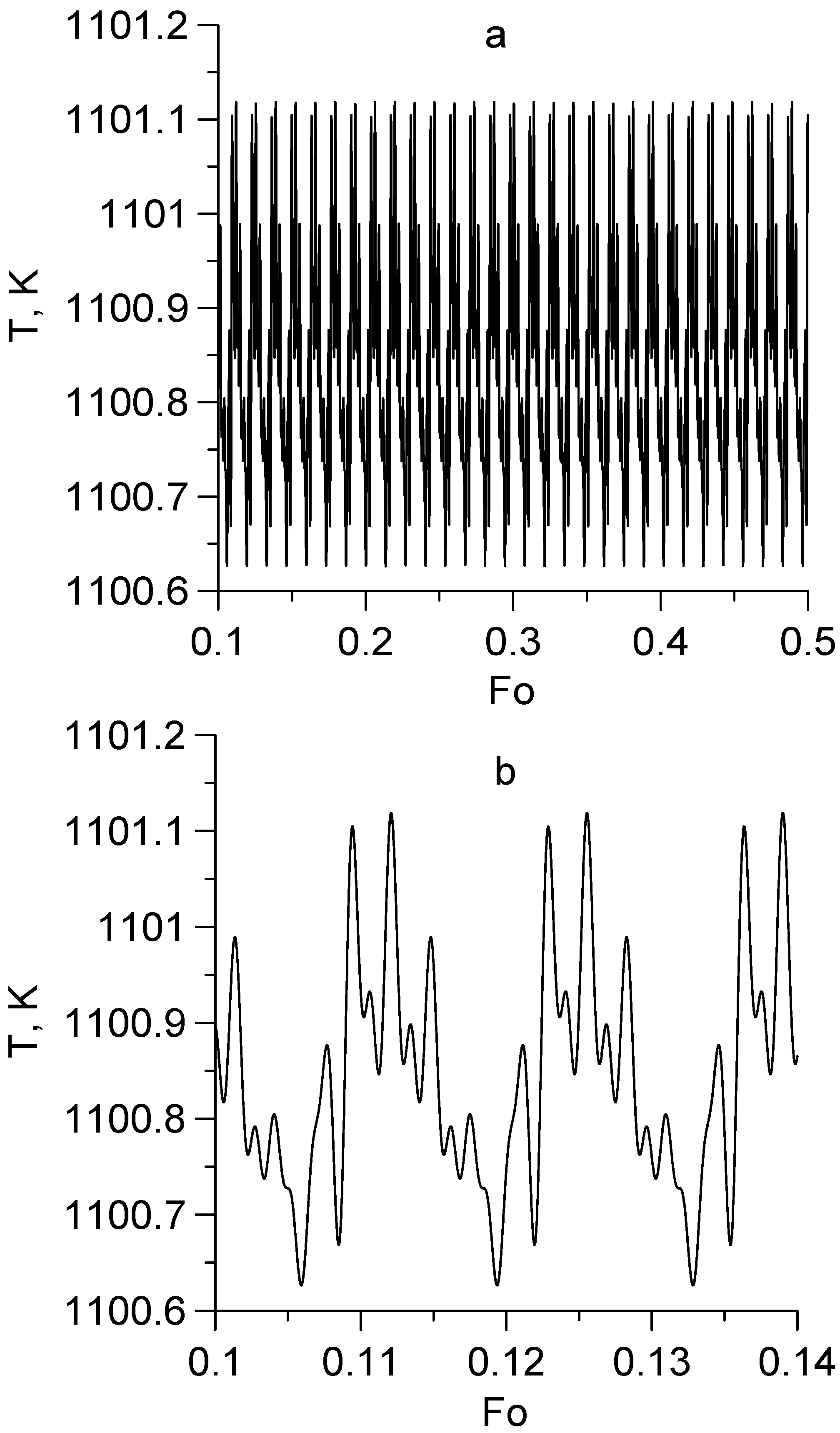
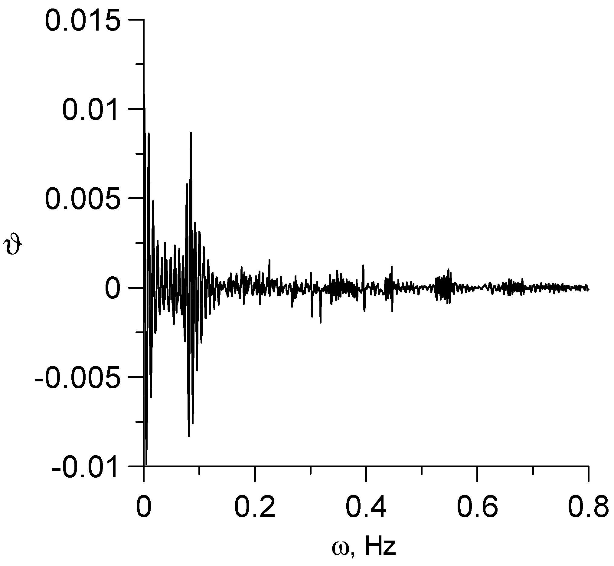
• The non-stationary temperature field in a reactor of finite length has a short-term transition period beyond which the temperature is quasi-stationary. The quasi-stationary part of the solution against a background of constant temperature contains quasi-harmonic oscillations, the amplitude of which is determined by the rotation period of the screw and the superposition of heat flows reflected on the thermally insulated side surfaces and on the flat surfaces of the reactor inlet and outlet, where heat exchange with the external environment takes place. The amplitude of these oscillations is very weak, of the order of 0.5 K, but these oscillations reflect the specifics of the screw action.
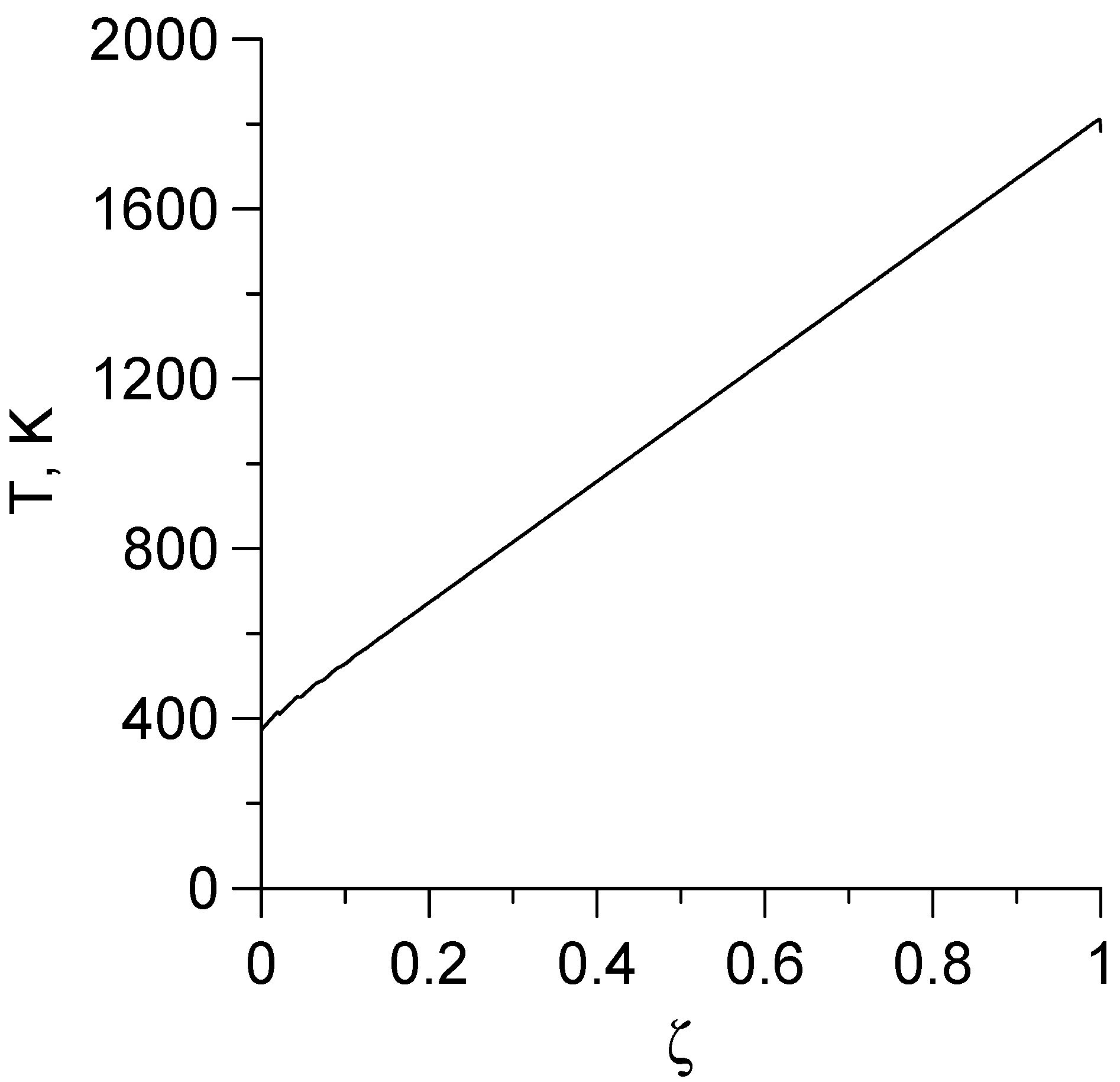
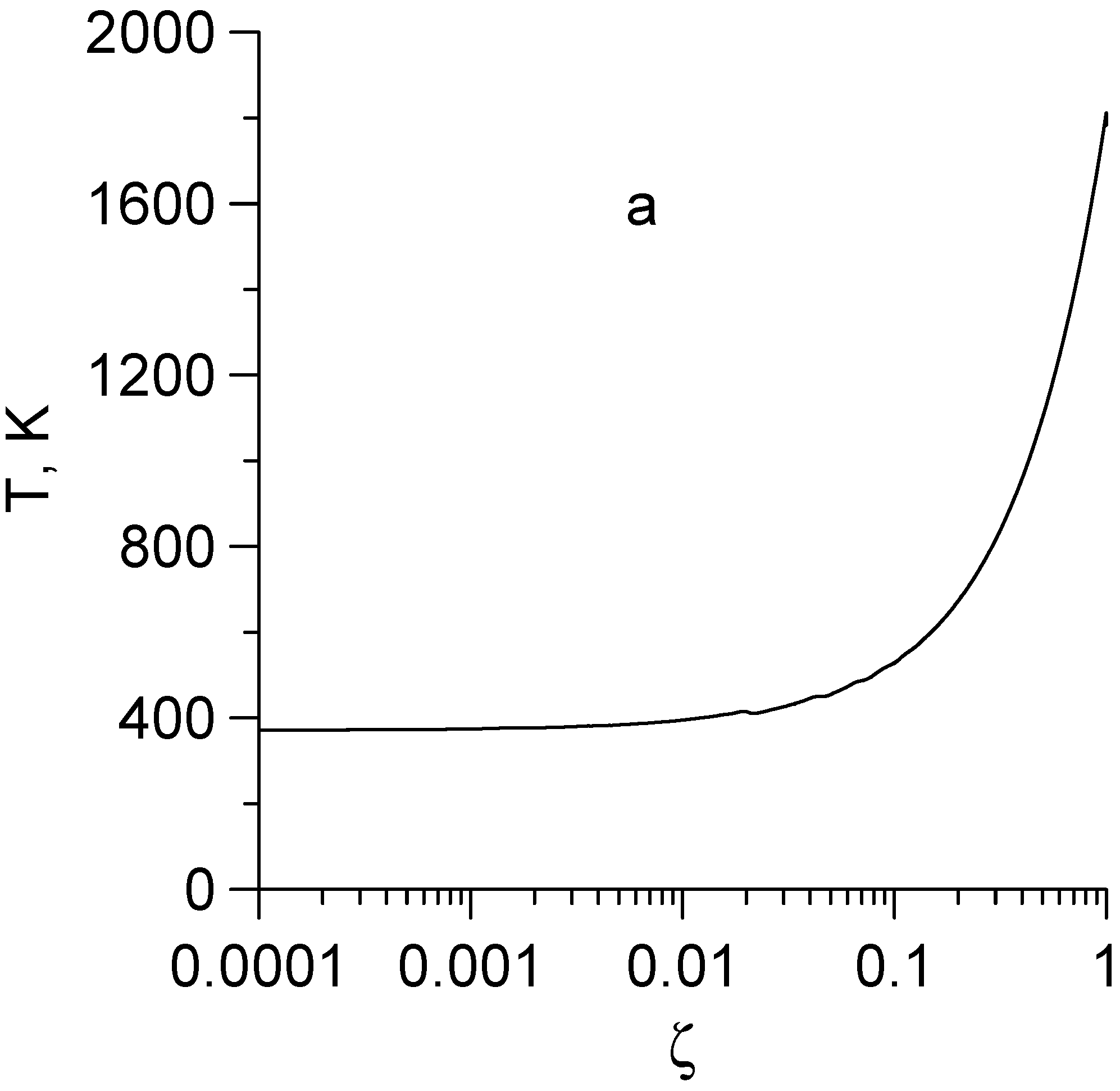
• Globally, the temperature is characterized by its increase along the screw axis in the direction of biomass linear movement. This effect, known from the experimental and theoretical literature [19,23,24], received a mathematical justification here. In addition, due to the movement of biomass, the solution of the problem has the character of a boundary layer, as a result of which the axial dependence of the temperature in the channel at a distance of the order of 1/b = 2a/v₀ from its entrance and exit has a slightly different form than on the main part of the reactor.
• Taking into account the speed of biomass movement leads to the emergence of a large parameter β = bL (of the order of 10³), which allows approximately summing a weakly convergent series by trigonometric functions and thereby regularizing solutions containing the exponent e^β multiplied by these series. Failure to use this procedure prevents numerical calculations. However, it should be noted that this is not the only method of regularization; other methods are also possible.
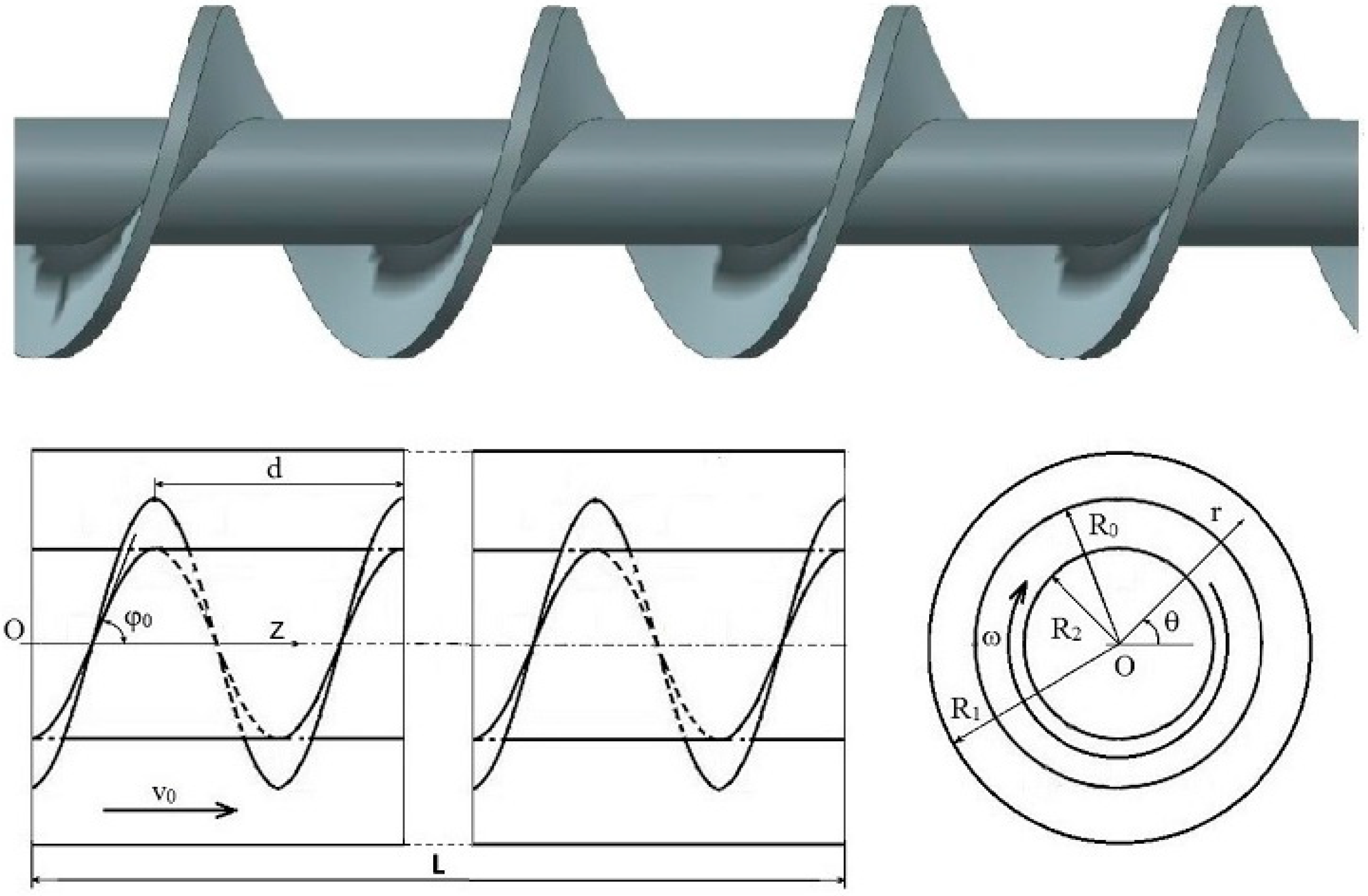
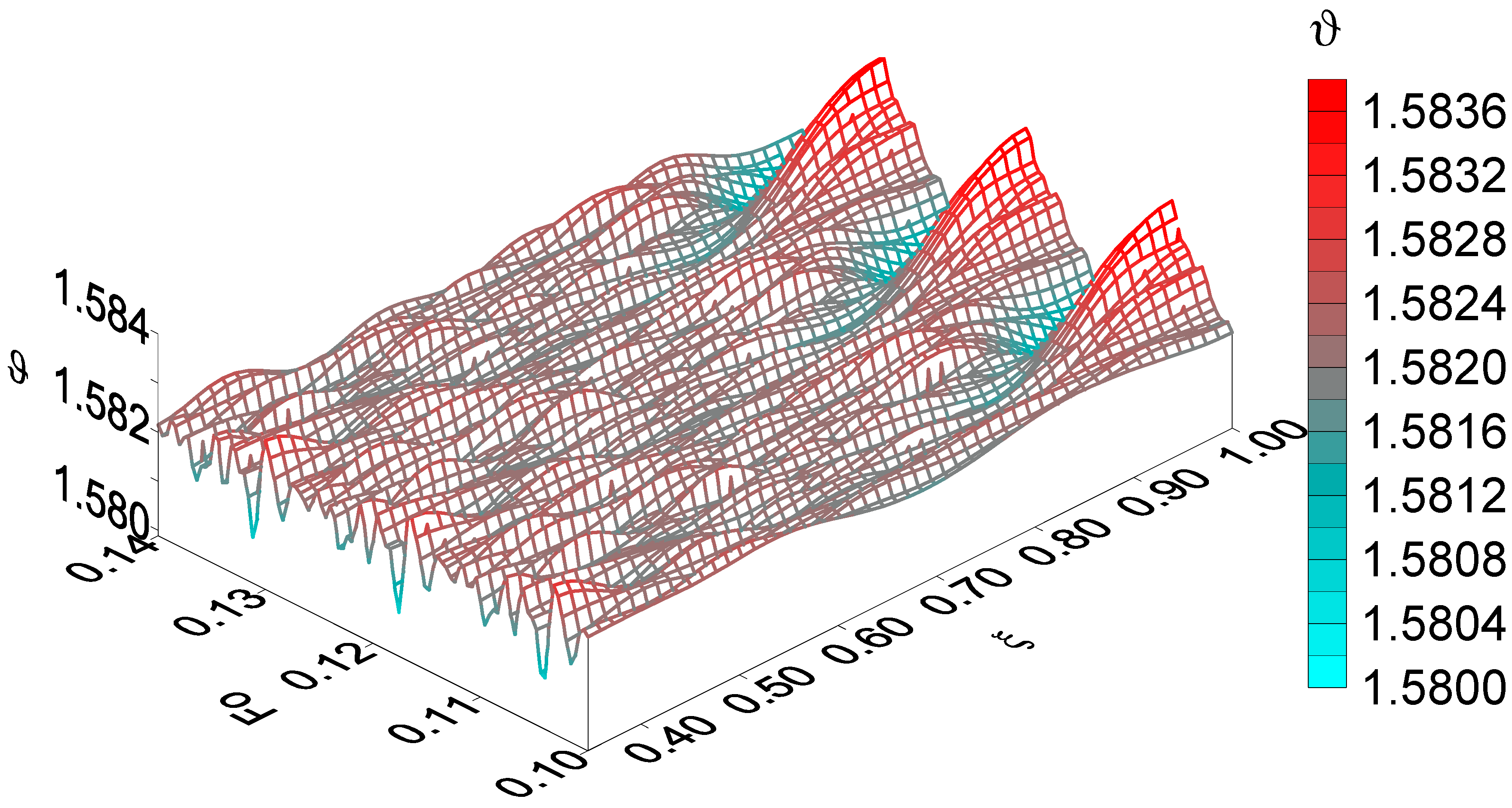
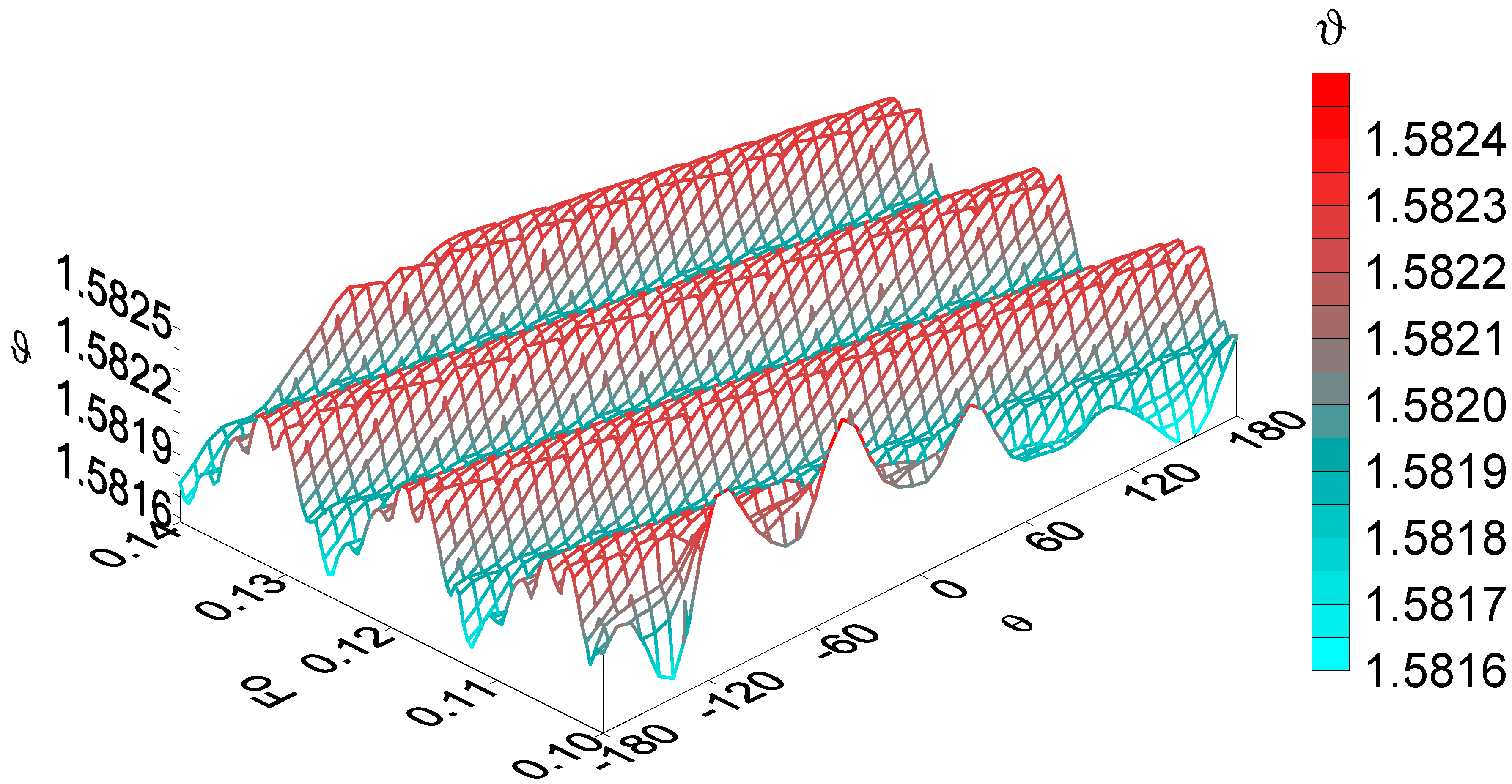
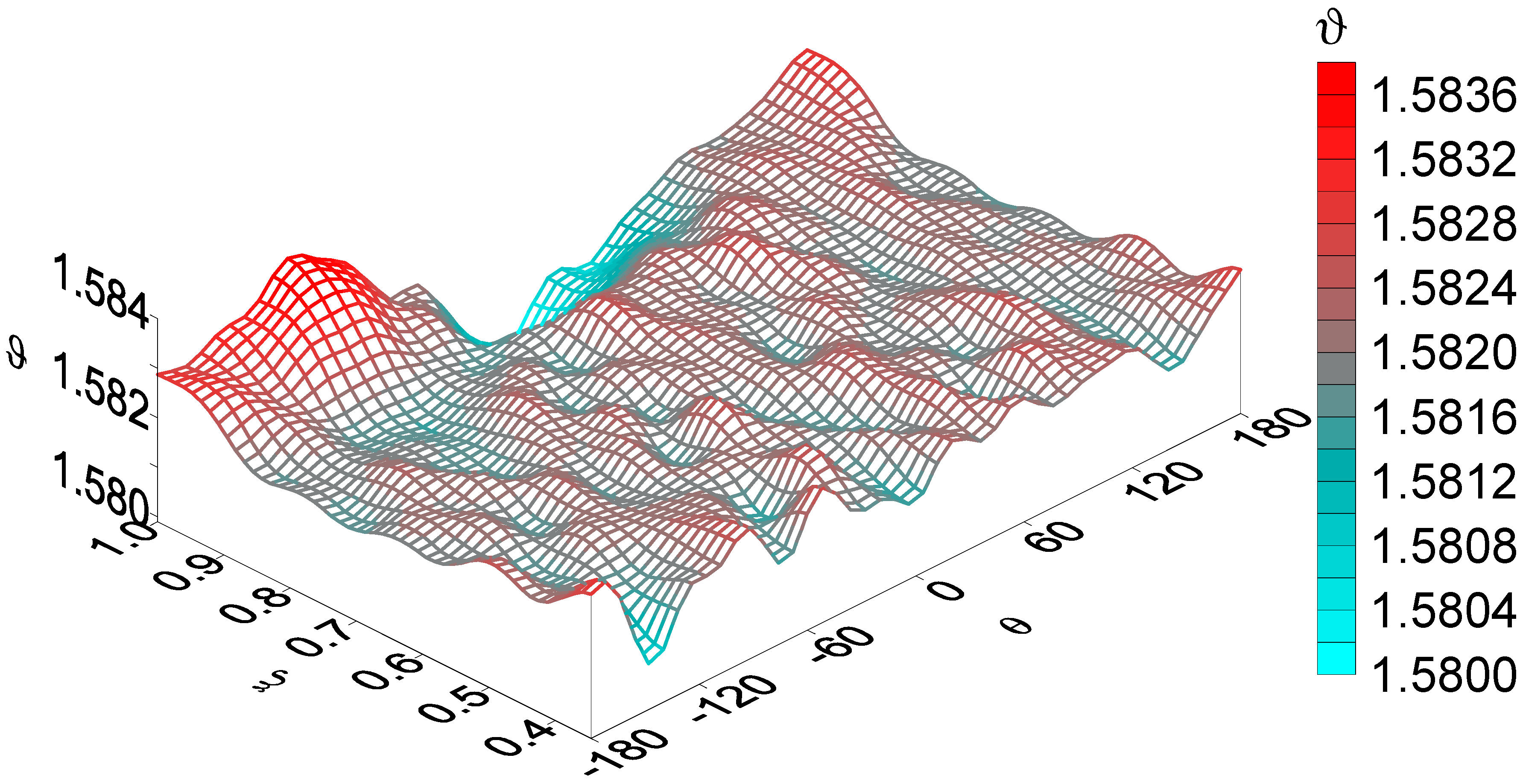
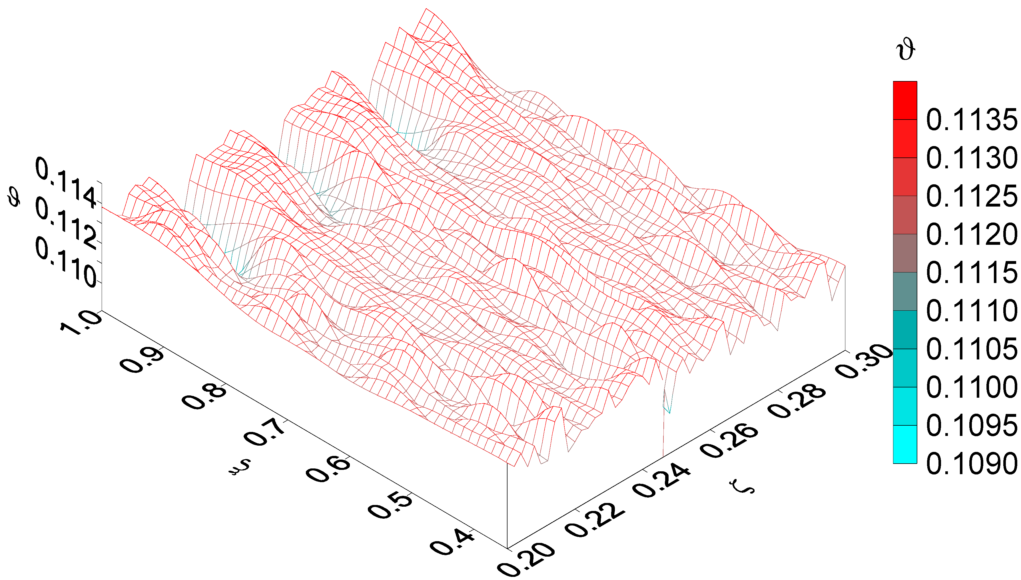
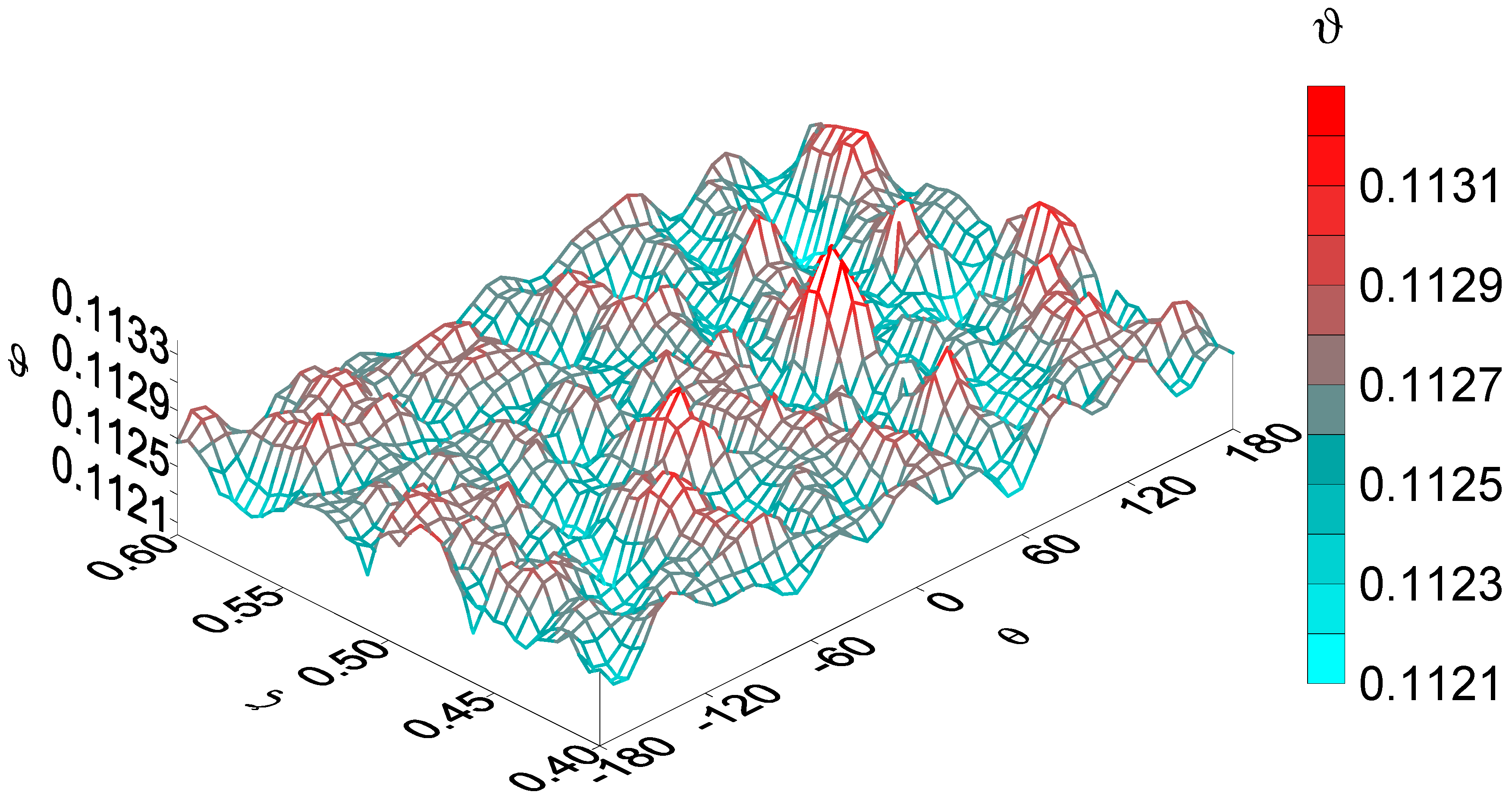
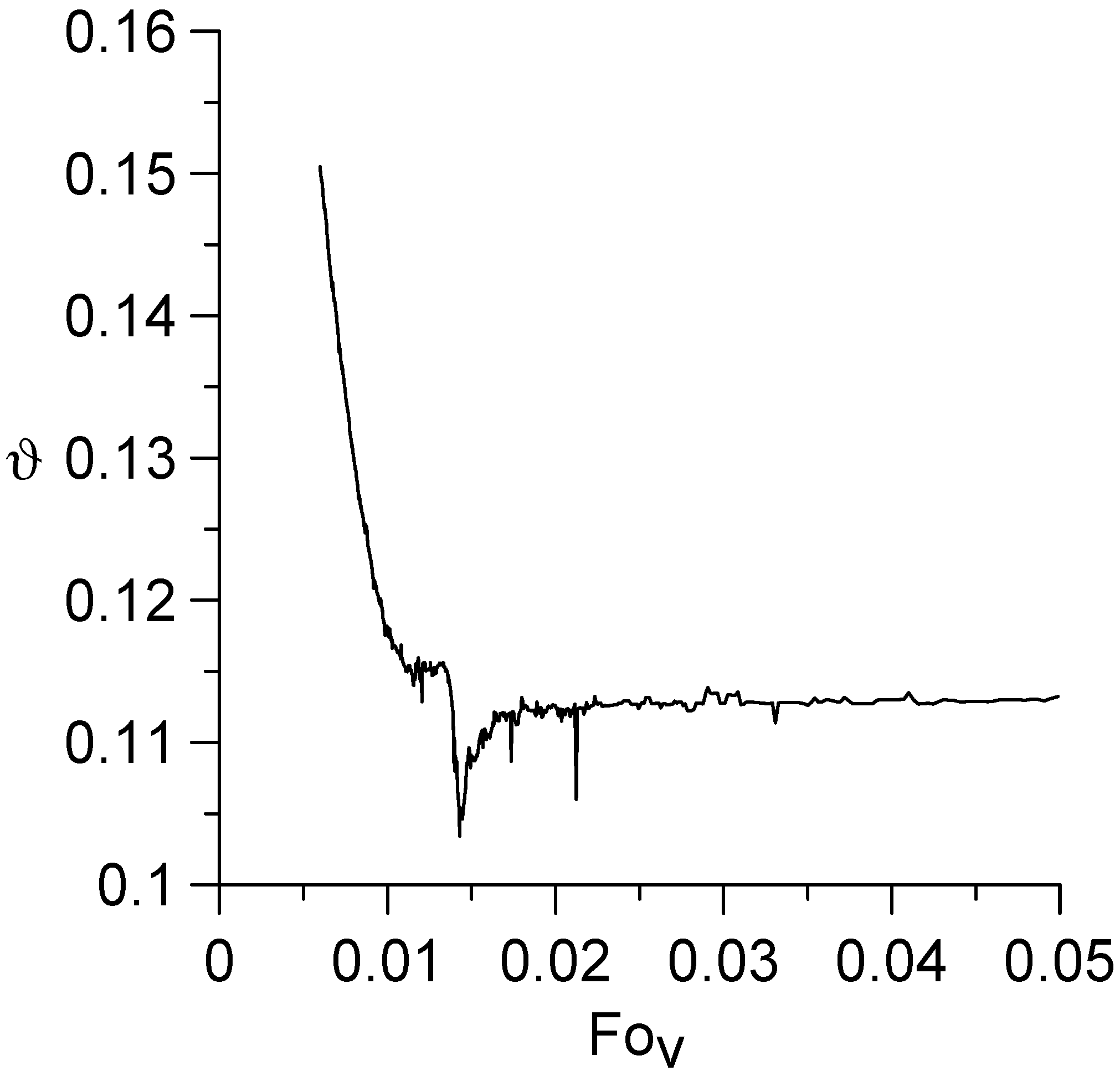
• This paper provides a detailed analysis of the sensitivity function ϑ, which depends only on the geometric and physico-mechanical parameters of the biomass and screw. It is shown that the change in time of this function is reflected in the form of the periodic appearance of spikes in the temperature amplitude. These spikes are arranged in space and time so that they reflect the shape of the screw. In particular, it was established that the temperature distribution in the radial direction is most sensitive to the geometry of the screw surface and its rotation frequency in those places of the filled reactor that are near the edge blades of the screw. The temperature has the same regular character in the angular direction. The most complex is the temperature field in the axial direction as a consequence of the complex superposition of heat flows.
• It is shown that as in the case of an infinitely long channel, for the temperature field in a channel of finite length, there is a condition of spatio-temporal resonance of the temperature field, under which, when the rotation frequency passes through a certain value associated with a constant speed of biomass movement, or vice versa, when the speed of biomass movement passes through a fixed value related to the angular speed of rotation of the screw, the temperature undergoes a sharp increase in the amplitude of oscillations and a sharp change in the phase of oscillations. However, due to interference effects in the case of a channel of finite length, this process is more complex in nature.
• Until now, practically nothing was known about the temperature field in such problems. We limited ourselves to a linear non-connected model of thermal conductivity of a moving substance with a moving heat source of complex shape. We tried to show what kind of spatial–dynamic distribution of the temperature field can be expected in a heating regime close to the one in which the experimentally observed biomass pyrolysis process takes place. The question of the adequacy of such a model for the problem of biomass processing can be solved by experimental measurements of the temperature field in space and time, for which, we hope, the results obtained here can be useful. Experience shows that it seems that the applicability of our results has limitations to the sterilization or pasteurization of food products. Unfortunately, corresponding temperature measurements are currently missing from the literature.

References

1. Campuzano, F.; Brown, R.C.; Martinez, J.D. Auger reactors for pyrolysis of biomass and wastes. Renew. Sustain. Energy Rev. 2019, 102, 372–409. [Google Scholar] [CrossRef]
2. Makavana, J.M.; Sarsavadia, P.N.; Chauhan, P.M. Effect of pyrolysis temperature and residence time on bio-char obtained from pyrolysis of shredded cotton stalk. Int. Res. J. Pure Appl. Chem. 2020, 21, 10–28. [Google Scholar] [CrossRef]
3. Solar, J.; de Marco, I.; Caballero, B.M.; Lopez-Urionabarrenechea, A.; Rodriguez, N.; Agirre, I.; Adrados, A. Influence of temperature and residence time in the pyrolysis of woody biomass waste in a continuous screw reactor. Biomass Bioenergy 2016, 95, 416–423. [Google Scholar] [CrossRef]
4. Yu, Y.; Yang, Y.; Cheng, Z.; Blanco, P.H.; Liu, R.; Bridgwater, A.V.; Cai, J. Pyrolysis of rice husk and corn stalk in auger reactor: Part 1. Characterization of char and gas at various temperatures. Energy Fuels 2016, 30, 10568–10574. [Google Scholar] [CrossRef]
5. Piersa, P.; Unyay, H.; Szufa, S.; Lewandowska, W.; Modrzewski, R.; Slęzak, R.; Ledakowicz, S. An extensive review and comparison of modern biomass torrefaction reactors vs. biomass pyrolysis—Part 1. Energies 2022, 15, 2227. [Google Scholar] [CrossRef]
6. Slęzak, R.; Unyay, H.; Szufa, S.; Ledakowicz, S. An extensive review and comparison of modern biomass torrefaction reactors vs. biomass pyrolysis—Part 2. Energies 2023, 16, 2212. [Google Scholar] [CrossRef]
7. Musii, R.; Pukach, P.; Kohut, I.; Vovk, M.; Šlahor, L. Determination and analysis of Joule’s heat and temperature in an electrically conductive plate element subject to short-term induction heating by a non-stationary electromagnetic field. Energies 2022, 15, 5250. [Google Scholar] [CrossRef]
8. SAFESTERIL: ETIA ECOTECHNOLOGIES a Branch of the ETIA Group. Available online: https://safesteril.etia-group.com (accessed on 22 June 2023).
9. Ledakowicz, S.; Stolarek, P.; Malinowski, A.; Lepez, O. Thermochemical treatment of sewage sludge by integration of drying and pyrolysis/autogasification. Renew. Sustain. Energy Rev. 2019, 104, 319–327. [Google Scholar] [CrossRef]
10. Ledakowicz, S.; Piddubniak, O. Analysis of non-stationary temperature field generated by a shaftless screw conveyor heated by Joule–Lenz effect. Chem. Process Eng. 2021, 42, 119–137. [Google Scholar] [CrossRef]
11. Piddubniak, O.P.; Piddubniak, N.G. Non-stationary temperature distribution in a thermally insulated concentric cylindrical channel with biomass moving under the influence of rotation of electrically heated helix. Math. Methods Physicomech. Fields 2021, 64, 107–123. (In Ukrainian) [Google Scholar] [CrossRef]
12. Piddubniak, O.; Ledakowicz, S. Modeling of heat transfer from an electrically heated rotating helix in a circular cylindrical channel filled with a biomass moving at a constant velocity. Therm. Sci. Eng. Prog. 2022, 30, 101265. [Google Scholar] [CrossRef]
13. Ledakowicz, S.; Piddubniak, O. The non-stationary heat transport inside a shafted screw conveyor filled with homogeneous biomass heated electrically. Energies 2022, 15, 6164. [Google Scholar] [CrossRef]
14. Carslaw, H.S.; Jaeger, J.C. Conduction of Heat in Solids; Clarendon Press: Oxford, UK, 1959. [Google Scholar]
15. Krein, S.G. (Ed.) Functional Analysis; Wolters-Noorhoff Publ.: Groningen, The Netherlands, 1972. [Google Scholar]
16. Tsoy, P.V. Methods for Calculating Heat Transfer Problems; Energoatomizdat: Moscow, Russia, 1984. (In Russian) [Google Scholar]
17. Luikov, A.V. Analytical Heat Diffusion Theory; Academic Press: New York, NY, USA, 1968. [Google Scholar]
18. Korn, G.A.; Korn, T.U. Mathematical Handbook for Scientists and Engineers: Definitions, Theorems and Formulas for References and Review; Dover Publ., Inc.: Mineola, NY, USA, 2000. [Google Scholar]
19. Gradshteyn, I.S.; Ryzhik, I.M. Table of Integrals, Series, and Products; Elsevier Inc.: Amsterdam, The Netherlands, 2007. [Google Scholar]
20. Nachenius, R.W.; Van De Wardt, T.A.; Ronsse, F.; Prins, W. Residence time distributions of coarse biomass particles in a screw conveyor reactor. Fuel Process. Technol. 2015, 130, 87–95. [Google Scholar] [CrossRef]
21. Shi, X.; Ronsse, F.; Roegiers, J.; Pieters, J.G. 3D Eulerian–Eulerian modeling of a screw reactor for biomass thermochemical conversion. Part 2: Slow pyrolysis for char production. Renew. Energy 2019, 143, 1477–1487. [Google Scholar] [CrossRef]
22. Fernández-Díaza, J.M.; Menéndez-Pérezb, C.O. A common framework for modified Regula Falsi methods and new methods of this kind. Math. Comput. Simul. 2023, 205, 678–696. [Google Scholar] [CrossRef]
23. Dahlquist, G.; Björck, Å. Numerical Methods in Scientific Computing; SIAM: Philadelphia, PA, USA, 2008; Volume 1. [Google Scholar]
24. Luz, F.C.; Cordiner, S.; Manni, A.; Mulone, V.; Rocco, V. Biomass fast pyrolysis in a shaftless screw reactor: A 1-D numerical model. Energy 2018, 157, 792–805. [Google Scholar] [CrossRef]
25. Yang, H.; Kudo, S.; Kuo, H.; Norinaga, K.; Mori, A.; Mašek, O.; Hayashi, J. Estimation of enthalpy of bio-oil vapor and heat required for pyrolysis of biomass. Energy Fuels 2013, 27, 2675–2686. [Google Scholar] [CrossRef]
Figure 1. The scheme of a screw of finite length with a shaft and the dimensions of its section.
Energies 16 06260 g001
Figure 2. The temperature at the point ξ = 0.5, θ = 0°, ζ = 0.5 at different values of the Fourier number Fo and current I.
Energies 16 06260 g002
Figure 3. The time dependence of the temperature (a) and its fragment (b) at the point ξ = 0.8, θ = 0°, ζ = 0.5 for I = 149 A.
Energies 16 06260 g003
Figure 4. Temperature distribution along the length of the channel (ξ = 0.8, θ = 0°, Fo = 0.5, I = 149 A).
Energies 16 06260 g004
Figure 5. Temperature distribution along the length of the channel near input to the channel (a) and near output from it (b) (ξ = 0.8, θ = 0°, Fo = 0.5, I = 149 A).
Energies 16 06260 g005aEnergies 16 06260 g005b
Figure 6. Sensitivity of the temperature field to boundary conditions (ξ = 0.8, θ = 0°, ζ = 0.5, Fo = 0.5, I = 149 A).
Energies 16 06260 g006
Figure 7. The radial–time dependence of the temperature on the ray ε0ξ ≤ 1, θ = 0°, ζ = 0.5 for the three periods of oscillation.
Energies 16 06260 g007
Figure 8. The angle–time dependence of the temperature on the circle ξ = 0.8, 0 ≤ |θ| ≤ 180°, ζ = 0.5 for the three periods of oscillation.
Energies 16 06260 g008
Figure 9. The axial–time dependence of the temperature on the circle ξ = 0.8, θ = 0°, 0.22 < ζ < 0.28 for the three periods of oscillation.
Energies 16 06260 g009
Figure 10. The 3D radial–angular instantaneous distribution of function θ in the cross-section ζ = 0.5 (Fo = 0.5).
Energies 16 06260 g010
Figure 11. The instantaneous radial–axial distribution of the function ϑ in the plane ε0ξ ≤ 1, 0 ≤ |ζ| ≤ 4 at θ = 0°, Fo = 0.5.
Energies 16 06260 g011
Figure 12. The 3D radial–angular instantaneous distribution of function θ in the cross-section ξ = 0.8 (Fo = 0.5).
Energies 16 06260 g012
Figure 13. The dependence of function ϑ on rotation frequency ω of screw at the point ξ = 0.8, θ = 0°, ζ = 0.5, Fo = 0.5 for φ0 = 73.68° and v0 = 5.89 × 10⁻⁴ m/s (Fov = 0.593).
Energies 16 06260 g013
Figure 14. The dependence of the influence function ϑ on Fourier number corresponding to the flow rate of the substance v0 at the point ξ = 0.8, θ = 0°, ζ = 0.5 for Fo = 0.5, φ0 = 73.68°, ω = 0.292 Hz (Fo0 = 0.0135) and R2 = 0.009 m.
Energies 16 06260 g014