Article

Research on Regional Carbon Emission Reduction in the Beijing–Tianjin–Hebei Urban Agglomeration Based on System Dynamics: Key Factors and Policy Analysis

1
School of Economics and Management, University of Chinese Academy of Sciences, Beijing 100190, China
2
School of Economics and Management, Beijing University of Chemical Technology, Beijing 100029, China
*
Author to whom correspondence should be addressed.
These authors contributed equally to this work.
Energies 2023, 16(18), 6654; https://doi.org/10.3390/en16186654
Submission received: 18 August 2023 / Revised: 9 September 2023 / Accepted: 13 September 2023 / Published: 16 September 2023
(This article belongs to the Collection Energy Transition towards Carbon Neutrality)

Abstract

:
Urban agglomerations are regions where the economy and population are highly concentrated, which are also spatial units with more concentrated carbon emissions. A detailed decomposition of driving factors based on changes in carbon emissions of urban agglomerations can provide a reference for better carbon reduction policies. In this paper, we establish an evaluation framework of carbon emission drivers of urban agglomeration from the perspective of CO2 generation and removal using a system dynamics method. The key influencing factors and optimal emission reduction measures of carbon emissions in urban agglomerations are explored. The results are as follows: (1) The industrial structure is the key influencing factor of carbon emissions; (2) compared with no implementation of any policies, the total carbon emissions and carbon emission intensity of integrated policies all significantly decrease, with a decrease of 43.68% and 53.32%, respectively in 2035; (3) energy structure adjustment has a significant effect in reducing carbon emissions and carbon emission intensity; (4) the role of increasing investment in technological innovation in ensuring achievement of “carbon peak” should not be ignored. It is found that integrated policies often exhibit a better emission reduction effect, but this effect is not a simple summation of the effects of each single policy.

1. Introduction

The current scale of change in the entire climate system and its status are unprecedented in hundreds or even thousands of years [1]. This has attracted widespread global attention, with the number of global media reports on “global warming” and “climate change” doubling since 2018 [2]. To mitigate the effects of climate change, numerous countries are taking active action. Until May 2021, 196 countries and regions had promulgated over 2315 laws and policies to address climate change [3]. In addition, many countries have announced that they will meet their carbon neutrality targets around 2050, such as Japan, Germany, and Canada [4]. In 2020, China also declared that it will achieve carbon peaking by 2030 and carbon neutrality by 2060 [5].
Guided by the global carbon reduction emission target, CO2 emission reduction measures have become the focus of research by scholars in various countries. Some scholars explored carbon emission reduction measures from a single macro policy perspective, such as energy policy [6,7], technology upgrading [8], carbon tax [9], and carbon emission trading policies [10,11,12]. However, it is difficult to explore the optimal emission reduction policy by considering only the regulatory impact of a single policy. So, some scholars considered different policies comprehensively and established various scenarios by regulating the economy, energy, and industrial structure to simulate and predict the impact of different policies on carbon emissions, and further analyzed the policy options with the greatest contribution to carbon emission reduction [13,14]. In addition, some scholars have studied the impact of urbanization [15], digital economy [16], and trade [17,18,19,20] on carbon emissions.
To explore the time point of carbon peaking and carbon neutrality, some scholars conducted research on carbon emission trend prediction. The main simulation forecasting methods can be divided into three major categories [21], namely indicator decomposition, scenario analysis, and system optimization. One of the most popular models adopted in the indicator decomposition method is the STIRPAT model. Wang et al. used the extended STIRPAT model to forecast and analyze the carbon peak time for nine subsectors of industrial industries in China [22]. Ofori et al. expanded upon the STRIPAT model to test the impact of environmental policies and eco–friendly innovations on carbon emission reduction [23]. For scenario analysis, the LEAP model is commonly used. Handayani et al. used the LEAP model to assess the measures to achieve net–zero emissions in the power sector of the Association of Southeast Asian Nations by 2050 [24]. For the system optimization method, the system dynamics model seemed to be favored by most scholars. Mirzaei et al. simulated Iran’s energy consumption and CO2 emission trends from 2000 to 2025 using a system dynamics model [25]. Other than these, methods such as the Grey model [26] and carbon Kuznets curve (CKC) [27] have also been applied for carbon peak time prediction.
It can be seen that most of the previous studies on carbon reduction measures and carbon peak time prediction focused on the national, provincial, or city level. However, studies on national or provincial emission reduction cannot effectively reflect the differences in different regions in terms of factors such as the level of economic and social development, industrial characteristics, and energy structure. The studies on emission reduction in single cities are too specific and have low generalizability. However, these problems can be well addressed by taking urban agglomerations as the level of study. Urban agglomerations are regions where the economy and population are highly concentrated, which are also spatial units with more concentrated carbon emissions. Urban agglomerations represent the most advanced level of economic and social development in each region, and they supposedly take the lead in achieving carbon peaking, providing a model and valuable example for other regions, which is the key to achieving carbon peaking at the regional level [28].
It is an important issue to develop carbon peaking plans and design carbon reduction measures fairly and effectively at the regional level. Some scholars have realized the importance of conducting research on emission reduction in urban agglomerations, but the number of studies is relatively limited. Fang et al. explored a carbon tax pilot in the Yangtze River Delta (YRD) urban agglomeration based on a new energy saving and emission reduction (ESER) system with carbon tax constraints [29]. Zhang et al. conducted an empirical analysis on the role of the spatial association of carbon emissions and carbon sinks in the Beijing–Tianjin–Hebei urban agglomeration at the national scale, using actual data from China from 2005 to 2017, through exploratory spatial data analysis and social network analysis. [30]. Lian et al. used continuous atmospheric CO2 monitoring, a new high-resolution near-real-time emission inventory, and an atmospheric Bayesian inverse model to quantify the timing and magnitude of daily emission reduction during the two lockdown periods in the Paris metropolitan area [31]. Wang et al. quantified the total factor carbon performance and carbon mitigation potential of 39 industrial sectors in the Beijing–Tianjin–Hebei urban agglomeration from 2010 to 2016 using a stochastic frontier approach [32].
The authors found that the existing research has several limitations: (1) Most of the studies focused on the national, provincial, or city level, and only a small number of studies focused on urban agglomerations. Exploring emission reduction measures in urban agglomerations can better provide a reference for achieving carbon reduction targets. (2) The existing studies on urban agglomerations quantitatively analyzed the effect of single-policy measures on carbon emission reduction, such as the carbon trading market and carbon tax, but it is difficult to explore optimal emission reduction measures. (3) Moreover, the existing studies on urban agglomerations only focused on carbon emissions considering several sectors in one urban agglomeration; this means that the model structures adopted are not refined and adaptable. Additionally, there is a lack of methodologies or research frameworks that could systematically and comprehensively analyze the drivers, future trends, and policy scenarios of carbon emissions in urban agglomerations. System dynamics (SD) can be an appropriate method to fill these gaps. The research on carbon emission reduction at the level of urban agglomerations involves multiple subjects and has multiple influencing factors. Compared with the other methods mentioned above, the SD method has the advantage of combining qualitative and quantitative analyses to solve complex problems and to better simulate the decision-making process as it is easy to associate observable patterns of behavior of a system with micro-level structures [33,34]. It can establish causal loops and feedback chains between different factors in a complex system to simulate the evolution of the system. In recent years, SD methods have been widely used for the analysis of carbon reduction measures at the national or urban level [35,36]. This field of research provides a better reference for this paper to explore carbon reduction measures of urban agglomerations.
This paper attempts to introduce SD methods into the study of carbon emission reduction in urban agglomerations. By taking the Beijing–Tianjin–Hebei urban agglomeration (BTHUA) as an example, the emission reduction measures of the urban agglomeration are explored, and carbon peak times are predicted. The characteristics of the BTHUA, such as the economic and social development characteristics, the primary sources of CO2 emissions, and the level of technological development, are taken into account. Then, the SD model of the CO2 emission mechanism of the BTHUA is built. The model contains five subsystems, namely the population and economy subsystem, the traffic subsystem, the industrial production subsystem, the electric power generation subsystem, and the carbon sink subsystem. After the validity of the model is verified with historical tests, the trend of CO2 emissions in the BTHUA from 2020 to 2035 is predicted. The SD theory is applied to explore the CO2 emission mechanism, and the key influencing factors of CO2 emissions are identified through sensitivity analysis. Finally, the effectiveness of different emission reduction scenarios (social development, industrial structure adjustment, energy structure adjustment, technological innovation investment, and an integrated scenario) is tested by setting the scenarios and introducing feedback. This paper also compares the impact of different scenarios on carbon emission trends and peak time from 2020 to 2035 and explores optimal emission reduction policies. The results are of great significance for exploring the optimal carbon emission reduction measures of urban agglomerations and provide a reference for policy formulation.
The contribution of this work is to provide an SD model for urban agglomerations that can systematically and comprehensively analyze the key influencing factors, future trends, and policy impacts of carbon emissions in urban agglomerations. In terms of case application, this study provides policy implications for the BTHUA to formulate more effective emission reduction policies. More importantly, this is an open platform that can be adjusted according to the needs of decision makers and can be applied to other urban agglomerations.
The rest of the paper is organized as follows: Section 2 introduces the study area and the SD model; Section 3 discusses the model simulation results, including sensitivity analysis and scenario analysis; and finally, Section 4 presents the conclusions and policy recommendations.

2. Methodology

2.1. Study Area

The BTHUA is a climate-sensitive and ecologically fragile area [37] and also one of the three fastest-developing urban agglomerations in China. As a major high-tech and industrial zone in China, the BTHUA is facing enormous pressure to reduce emissions due to its huge energy demand and rapid growth in carbon emissions [38]. At present, the energy consumption structure of the BTHUA is dominated by fossil fuels, especially coal, with a low proportion of clean energy consumption. During the period from 2010 to 2017, fossil energy consumption accounted for over 88% of the total energy consumption in the BTHUA, which is nearly 24 percentage points higher than the national average [39].

2.1.1. BTHUA Carbon Emission Status

The BTHUA’s carbon emission data for 2010–2019 were derived from the Beijing, Tianjin, and Hebei Provincial Bureau of Statistics (BTHBS) and are shown in Figure 1. The sources of carbon emissions in the BTHUA mainly include five aspects: traffic, industrial production, electric power generation, residents, and others. The BTHUA in industrial production includes the smelting and pressing of ferrous metals, nonmetal mineral products, coal mining and dressing, raw chemical materials and chemical products, and petroleum processing and coking. The proportion of carbon emissions in industrial production has always remained the highest, with an average proportion of 49.40% over the past decade, which is still growing. In terms of electric power generation, it mainly includes the production and supply of electricity, steam, and hot water. The average carbon emissions from electric power generation during the decade under study accounted for 37.23%, only second to industrial production. In addition, traffic and residents are also the main sources of CO2 generation in the BTHUA. The BTHUA agriculture and services produce a relatively low share of CO2, which are collectively classified in this paper as other sectors.

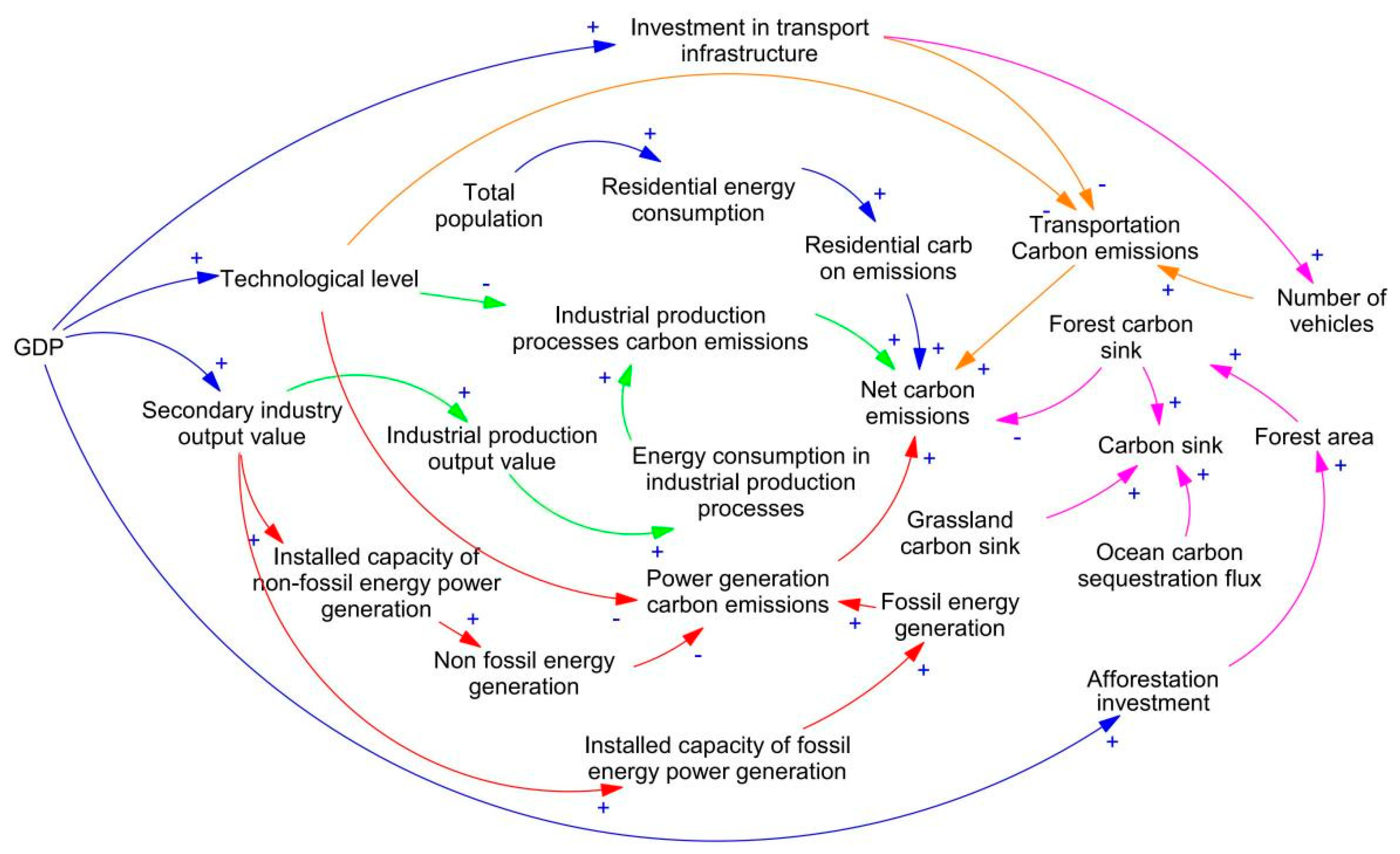
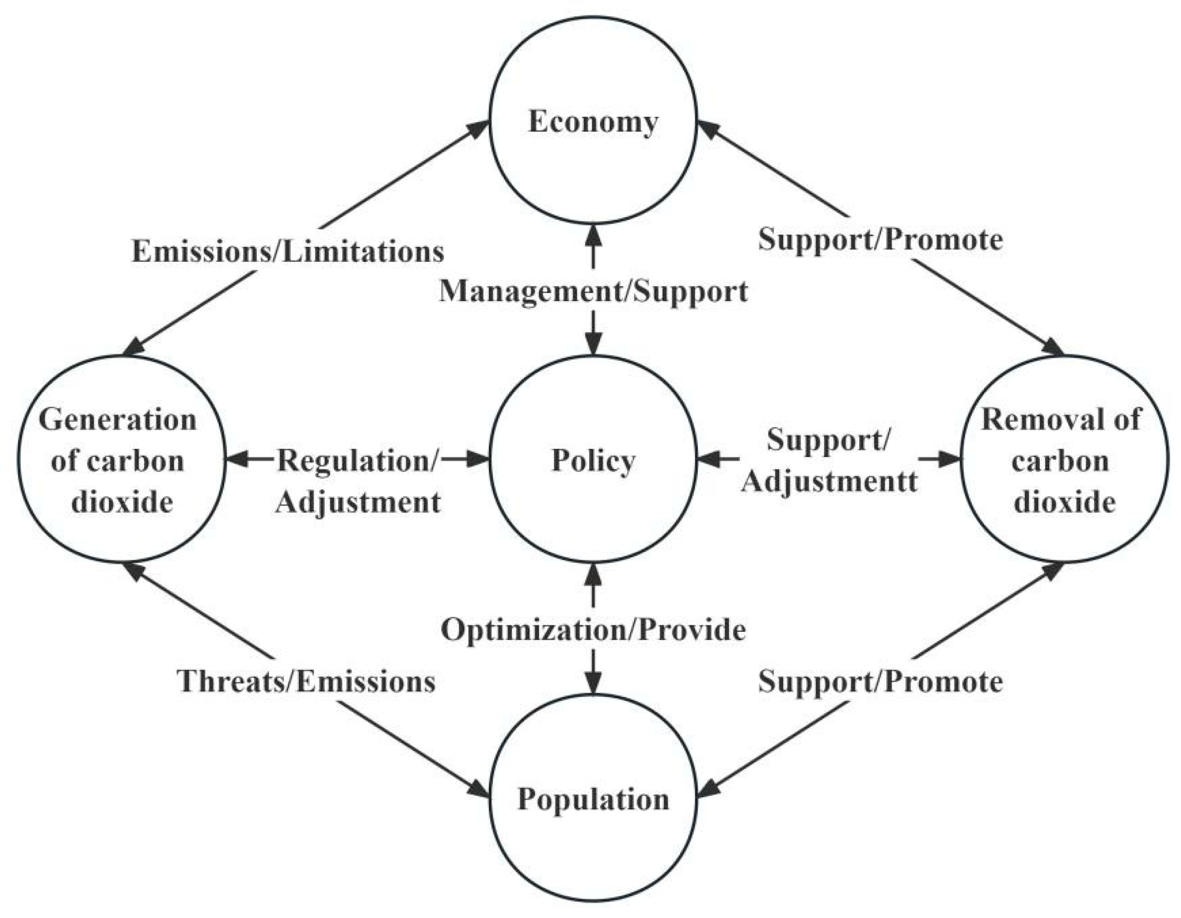
2.2. Model Structure

According to the IPCC definition, the generation of CO2 is mainly the result of human activities in the process of fossil fuel combustion, industrial production, agriculture, land use, etc. CO2 removal mainly involves carbon capture and afforestation to absorb CO2 from the atmosphere. Section 2.1.1 provides a detailed analysis of the sources of CO2 generation in the BTHUA. The removal of CO2 mainly involves carbon sinks, which include forest carbon sinks, grassland carbon sinks, and marine carbon sinks. Through the above analysis, we identified the influencing factors of carbon emissions and divided them into five subsystems: economy and population, traffic subsystem, industrial production, electric power generation, and carbon sink. Figure 2 (different colors of arrows represent different subsystems) selectively highlights the interactions between each subsystem. In addition, we reveal the constraints and feedback of carbon emission reduction policies in terms of both generation and removal, as shown in Figure 3. The amount of CO2 generated minus the amount of CO2 removed is equal to the net carbon emissions [40]. Carbon emission reduction targets are set according to the development plan of urban agglomerations or by reference to the development level of developed countries. There are several ways to control the gap between carbon targets and actual emissions. On the one hand, carbon emission reduction can be achieved through traditional methods such as updating environmental protection equipment or improving management efficiency. On the other hand, carbon emissions can be regulated by increasing the number of carbon sinks.

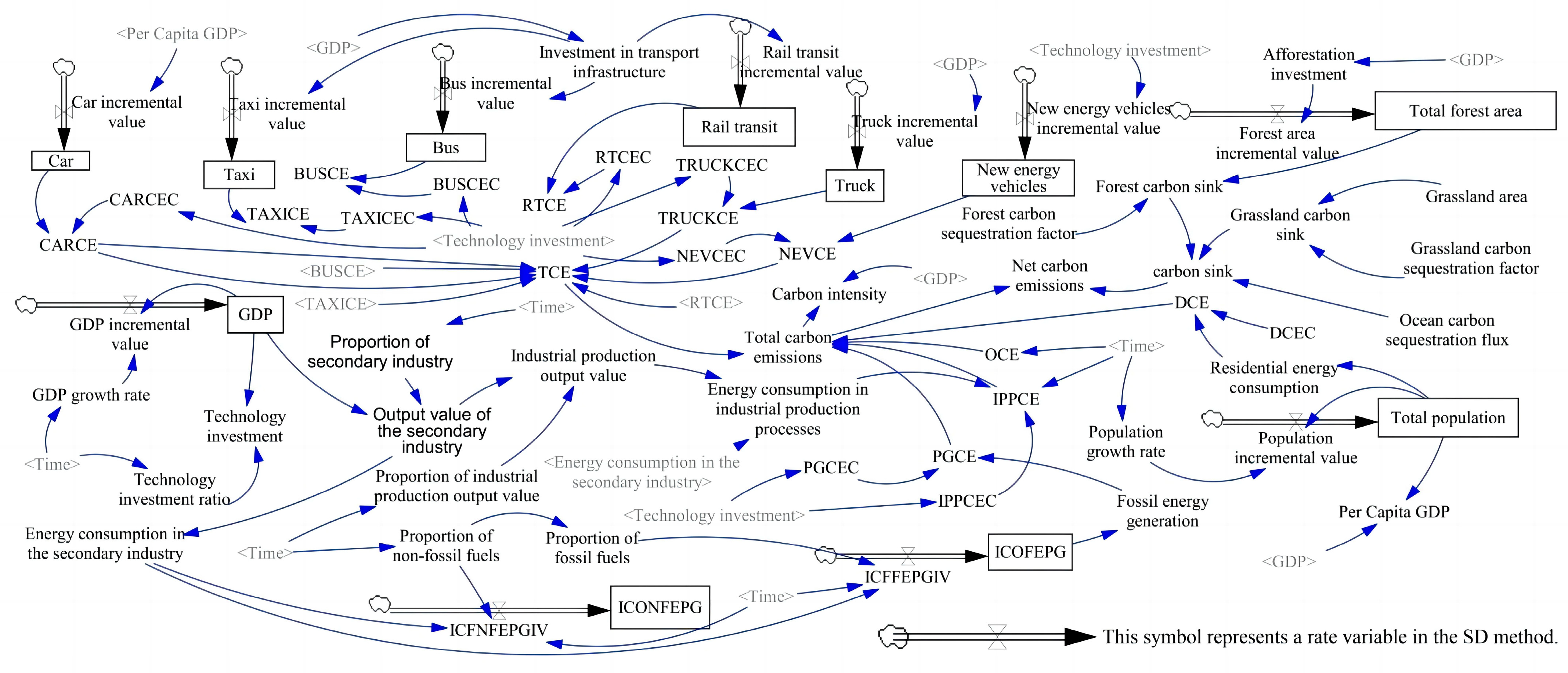
2.3. Flow Diagram Description

On the basis of the causal loop diagram, a carbon emission SD model of the BTHUA was drawn, as shown in Figure 4. In addition, Appendix A presents the equations of the SD model, as detailed in Table A1.

2.3.1. Economic and Population Subsystem

The economic and population subsystem mainly involves the analysis of the impact of economic growth and population growth on carbon emissions. The main variables include “GDP”, “GDP growth rate”, “total population”, “per capita GDP”, etc.
Total population = INTEG (Population incremental value, 104.55)
GDP = INTEG (GDP incremental value, 39,798.40)
The “total population” is the accumulation of “population increment”, with the initial value derived from the population data of the 2010 BTHBS (104.55 million), in which the “population increment” is determined by the “population growth rate”.

2.3.2. Traffic Subsystem

Traffic is one of the main sources of carbon emissions, and this subsystem mainly involves the analysis of the impact of changes in the number of different vehicles on carbon emissions. This subsystem mainly considers six vehicle models, namely car, taxi, bus, rail transit, truck, and electric vehicle.
Car = INTEG (Car incremental value, 9,287,400)
Car incremental value = 1.98481 × Per capita GDP + 1.38588 × 10⁶
TCE = BUSCE + TAXICE + TRUCKCE + NEVCE + CARCE + RTCE
The total number of cars is the accumulation of “car incremental value”, with the initial value derived from data from the National Bureau of Statistics of China (NBSC) in 2010 (9,287,400 vehicle units). The “car incremental value” is determined by the “per capita GDP”, and its equation is obtained through regression calculation. The “car carbon emission” (CARCE) value is the product of the “car carbon emission coefficient” (CARCEC) and “cars”. The CARCEC is calculated based on the carbon emission data of cars in the NBSC from 2010 to 2019. In addition, the “bus carbon emission coefficient” (BUSCEC), “taxi carbon emission coefficient” (TAXICEC), “truck carbon emission coefficient” (TRUCKCEC), “new energy vehicle carbon emission coefficient” (NEVCEC), and “rail transit carbon emission coefficient” (RTCEC) are all calculated from the carbon emission data of vehicles in the NBSC from 2010 to 2019. The “Traffic carbon emission” (TCE) variable represents the total carbon emissions of various types of transportation vehicles (TAXICE represents taxi carbon emissions, BUSCE represents buses carbon emissions, TRUCKCE represents truck carbon emissions, NEVCE represents new energy vehicle carbon emissions, and RTCE represents rail transit carbon emissions).

2.3.3. Industrial Production Subsystem

The industrial production subsystem mainly describes the carbon emissions generated during the industrial production process.
Energy consumption in industrial production processes = 0.245 × Industrial production output value + 0.764 × Energy consumption in the secondary industry
IPPCE = IPPCEC × Energy consumption in industrial production processes
The “energy consumption of industrial production processes” is determined by the “industrial production output” and the “energy consumption in the secondary industry”, and its equation is obtained through regression calculation. The “proportion of secondary industry” can directly affect the “industrial production output value” and “energy consumption in the secondary industry”. The variable “industrial production processes’ carbon emissions” (IPPCE) is the product of the “industrial production process carbon emission coefficient” (IPPCEC) and “energy consumption in industrial production processes”. The IPPCEC is calculated from the industrial production carbon emission data of the BTHBS from 2010 to 2019.

2.3.4. Electric Power Generation Subsystem

The effect of energy structure adjustment on carbon emission is studied by considering fossil energy and non-fossil energy.
ICOFEPG = INTEG (ICFFEPGIV, 65.98)
ICONFEPG = INTEG (ICFNFEPGIV, 0)
PGCE = Fossil energy generation × PGCEC
The “installed capacity of fossil energy power generation” (ICOFEPG) is the accumulation of “installed capacity for fossil energy power generation incremental value” (ICFFEPGIV). Considering the availability of data, the initial value of this variable is derived from the 2015 China Electric Power Yearbook (65.98 million KW), and the ICFFEPGIV is determined by the “energy consumption in the secondary industry” and the “proportion of fossil fuels”. The “installed capacity of non-fossil energy power generation” (ICONFEPG) is the accumulation of “installed capacity for non-fossil energy power generation incremental value” (ICFNFEPGIV), with an initial value obtained from the data on clean energy power generation (wind power, hydropower, nuclear power, etc.) recorded in the 2015 China Electric Power Yearbook (0 KW). Using these data, the ICFNFEPGIV is determined by the “energy consumption in the secondary industry” and the “proportion of non-fossil fuels”. The variable “power generation carbon emissions” (PGCE) is the product of the “power generation carbon emission coefficient” (PGCEC) and “fossil energy generation”, and the PGCE is calculated based on carbon emission data from BTHBS from 2010 to 2019.

2.3.5. Carbon Sink Subsystem

The role of carbon sinks is to remove CO2 from the atmosphere, mainly comprising forest carbon sinks, grassland carbon sinks, and marine carbon sinks.
Forest carbon sink = Forest carbon sequestration factor × Total forest area
Grassland carbon sink = Grassland carbon sequestration factor × Grassland area
Carbon sink = Forest carbon sink + Grassland carbon sink + Ocean carbon sequestration flux
The “forest carbon sink” is the product of the “forest carbon sequestration factor” and “total forest area”. The “total forest area” is determined by “afforestation investment”, and the “total forest area” increases with the increase in “afforestation investment”. The “forest carbon sequestration factor” and “grassland carbon sequestration factor” are derived from the 2006 IPCC report, and the “ocean carbon sequestration flux” is derived from the literature [13].

2.4. The BTHUA Data

The main data sources of this paper are from the China Statistical Yearbook, the China Environmental Statistical Yearbook, BTHBS, China Electric Power Yearbook, and NBSC from 2010 to 2019.

2.5. Model Test

To ensure that the model can accurately reflect the trends of carbon emissions in the BTHUA, it is necessary to test the rationality and applicability of the model after establishing it. Historical tests can determine whether the model is effective by comparing the differences between the simulation data and the historical data of each variable [41]. Therefore, we conducted a historical test on the main variables of the model under the baseline scenario (BS). These variables include the “GDP”, the “total population”, and the “total carbon emissions”, among which the “GDP” and the “total population” are the main output variables of the economy and society, and are closely related to other subsystems. The variable denoted as “total carbon emissions” is the main evaluation indicator in this study and is an important variable to reflect the effectiveness of emission reduction. Some other related studies have also pointed out that the validation of these variables can effectively reflect the accuracy and credibility of the model [42]. Considering the accessibility of historical data, the starting year for historical testing was 2010 and the ending year was 2019. The specific test results are shown in Table 1. The results show that the development trend of the variable simulation data is consistent with that of the historical data, and the relative errors are within 10%. Therefore, the model can effectively reflect the actual situation of carbon emissions in the BTHUA.

2.6. Evaluating Key Influencing Factors Based on Sensitivity Analysis

To ensure the effectiveness of the model, sensitivity analysis is necessary to test the model’s response to input variables and explore the key influencing factors of carbon emissions in the BTHUA [43]. Based on the analysis of the influencing factors of carbon emissions, we used the SD method to select the five main influencing factors for sensitivity analysis, namely GDP, population, industrial structure, energy structure, and technology investment. To analyze and compare the effects of these influencing factors on carbon emissions, some influencing factors were changed at the same rate (±10%), while other variables were kept constant. Analyzed from the literature review and empirical research on carbon emission reduction in the BTHUA, these five variables may be the main factors directly affecting carbon emissions. Moreover, the studies of Yang et al. [42] and Li et al. [44] also provide a reference and basis for the selection of variables in the sensitivity analysis of this paper. On this basis, by analyzing the degree of impact of various factors on carbon emissions, the key influencing factors were identified. For this reason, we set four scenarios other than the BS, and the specific adjustment parameters are shown in Table 2.

2.7. Scenario Settings

There is a lack of policy research on carbon emission reduction in urban agglomerations. However, relevant policy objectives can refer to provincial policies to a certain extent. At present, the number of policies related to carbon peaking and carbon emission reduction issued by China reaches 210, and the content of the policies mostly focuses on programs aiming to achieve carbon peaking and carbon neutrality, scientific and technological innovation support, carbon reduction in key industries or fields, energy efficiency constraints, energy saving and emission reduction, etc. The existing studies have also analyzed the key factors affecting carbon emission reduction, such as social development [45], industrial structure [21], energy structure [46], and technological innovation [47].
Based on the carbon emission model of the BTHUA, we set the following five emission reduction scenarios according to the development plan of the urban agglomeration and the development level of developed countries to explore the optimal emission reduction policies and analyze the impact of different policies on the carbon emission trend and the carbon peak time of urban agglomerations. The specific parameter settings are shown in Table 3.
Social Development Scenario (SDS): This scenario aims to reduce carbon emissions by accelerating socio-economic development. Under this scenario, policy objectives focus on population and economic growth and do not give much consideration to changing the industrial and energy structure or increasing the proportion of investment in science and technology. The outline of the BTH Coordinated Development Plan proposes that the BTHUA should become an important region with strong international competitiveness and influence by 2030 and even be able to lead and support national economic and social development. At the same time, considering the slow decline in economic growth in developed countries and referring to the research by Dai et al. [45], we simulated the trend of carbon emissions under SDS by adjusting the “GDP growth rate” and the “population growth rate”.
Industrial Structure Adjustment Scenario (ISAS): This scenario aims to reduce carbon emissions by adjusting and optimizing the industrial structure. Under this scenario, the policy objectives focus on the optimization of the industrial structure, and economic growth is appropriately slowed down, while the energy structure and investment in science and technology are not significantly changed. Since the beginning of the industrial era, carbon emissions from fossil fuels have continued to grow. Xiang and Xu [21] pointed out that structural reform is a key way to achieve carbon reduction targets in the short term. We also considered the proportion of the secondary industry after the “three industrialization stages” in developed countries such as the United States to adjust the industrial structure and simulate the trend of changes in carbon emissions under the ISAS.
Energy Structure Adjustment Scenario (ESAS): This scenario aims to reduce carbon emissions by adjusting and optimizing the energy structure. Under this scenario, the policy objectives focus on the optimization of the industrial structure, and economic growth slows down appropriately, while the industrial structure and the proportion of scientific and technological inputs are not changed significantly. Working Group I of the IPCC’s sixth assessment report stated that, between 2010 and 2019, the average carbon emissions from fossil fuels reached 9.6 ± 0.5 PgC yr−1, accounting for 86% of all anthropogenic carbon emissions. At the same time, in 2020, the China Energy and Power Development Outlook issued by the State Grid Energy Research Institute projected that, by 2035, China’s non–fossil energy consumption will account for 40% of primary energy consumption. Taking this as a reference, by adjusting the proportion of non-fossil fuels to change the energy structure, we simulated the trend of carbon emissions under the ESAS.
Technological Innovation Scenario (TIS): This scenario aims to reduce carbon emissions by increasing investment in science and technology. Under this scenario, the policy objectives focus on increasing investment in science and technology, and economic growth slows down appropriately, while the industrial and energy structures do not change significantly. Technology investment can promote technological innovation and equipment upgrading, thereby improving energy utilization efficiency and effectively reducing carbon emissions. In recent years, the investment in innovation funds in the BTHUA has continued to increase, placing greater emphasis on basic research. In this scenario, we referred to the average proportion of “R&D investment” in Beijing from 2010 to 2019 and adjusted the “technology investment ratio” to simulate the trend of carbon emissions under the TIS.
Integrated Scenario (IS): This scenario aims to integrate various measures to reduce carbon emissions. Taking into account four aspects, namely economic and population growth, industrial structure adjustment, energy structure adjustment, and increased investment in technology, we simulated the changing trend of carbon emissions under the IS.

3. Empirical Results and Analysis

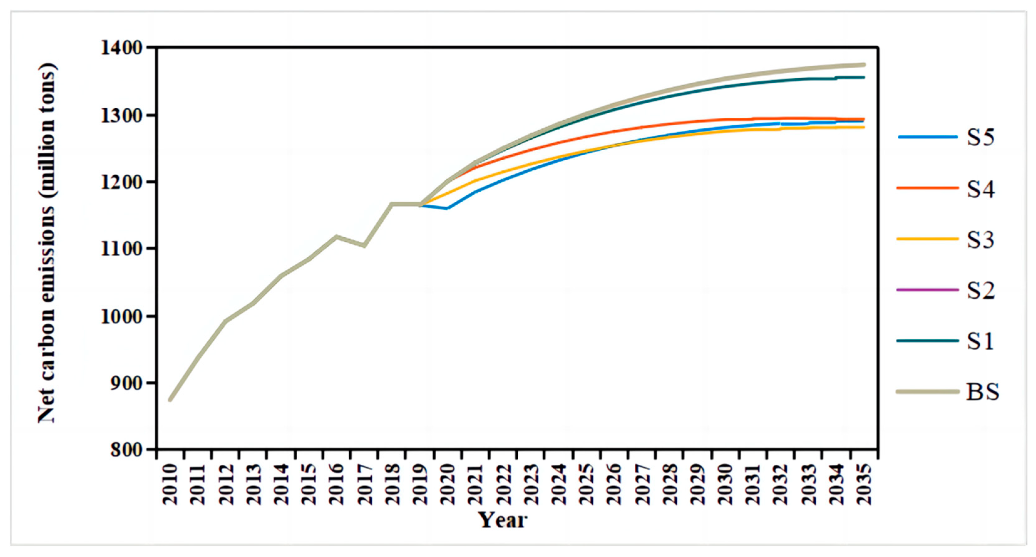
3.1. Results of Sensitivity Analysis and Key Influencing Factors

This study involves a sensitivity analysis method based on SD to evaluate the key influencing factors of carbon emissions in the BTHUA. We evaluated and compared the impact of different factors on future carbon emissions by controlling the same rate of change. The results are shown in Figure 5.
The simulation results indicate that economic growth can reduce carbon emissions to some extent. Compared with the BS, when the economic growth rate increases by 10%, the net carbon emissions will decrease by 1.27% in 2035. However, this situation does not reach its peak in the simulation time (i.e., 2010–2035). This is different from the results on the impact of economic growth on carbon emissions obtained by Jia et al. [48]. The main reason for this is that Jia et al. [48] did not take into account the relationship between economic growth and investment in technological innovation and afforestation. The results of this study show that economic growth can reduce carbon emissions by increasing investment in technology, infrastructure, afforestation, and other aspects.
Population growth has a positive impact on carbon emissions, but the degree of impact is relatively limited. Compared with the BS, when the population growth rate increases by 10%, the net carbon emissions will increase by 0.05% in 2035. The results indicate that rapid population growth will put pressure on the environment, which is consistent with the results obtained by Qin et al. [49]. This is mainly due to the continuous growth of residents’ energy consumption with the increase in population, which further leads to an increase in carbon emissions from daily life.
Industrial structure adjustment can significantly reduce carbon emissions. Compared with the BS, when the proportion of the secondary industry decreases by 10%, the net carbon emissions will decrease by 6.80% in 2035. Carbon emissions will peak in 2034, with a carbon peak amount of 1281.29 million tons. Over the past decade, industrial production has been the main source of carbon emissions in the BTHUA. Therefore, by adjusting the industrial structure and reducing the proportion of the secondary industry, carbon emissions can be significantly reduced. Some other studies on the national level also reveal that industrial structure adjustment has a significant impact on carbon emission reduction [42]. This is consistent with the finding of Xiang and Xu indicating that industrial structure is the first contributor to global carbon emission reduction [21].
Energy structure adjustment can effectively reduce carbon emissions. Compared with the BS, when the proportion of non-fossil fuels increases by 10%, the net carbon emissions will decrease by 6.03% in 2035. Carbon emissions will peak in 2032, with a carbon peak amount of 1294.99 million tons. In addition, as energy consumption is the direct source of CO2 generation, reducing fossil energy consumption and increasing the use of clean energy such as wind power and hydropower can effectively reduce carbon emissions and advance the time of carbon peaking.
Increasing investment in technological innovation can effectively reduce carbon emissions. Compared with the BS, when the proportion of technology investment increases by 10%, the carbon emissions will decrease by 6.13% in 2035. However, this situation does not reach its peak during the simulation time. Increasing investment in technological innovation, improving CCUS and other technologies, achieving efficient and clean utilization of fossil fuels such as coal, and further measures to reduce carbon emissions from coal-fired power plants can effectively reduce carbon emissions. This is consistent with the findings of Jia et al. [48].
In summary, population growth has a relatively limited impact on carbon emissions, and economic growth can affect carbon emissions to some extent. The impact of industrial structure adjustment, energy structure adjustment, and technological innovation investment on carbon emissions is relatively significant. Based on the simulation results of sensitivity analysis, and combined with the characteristics of carbon emissions in the BTHUA, it is found that industrial structure adjustment has the most significant driving effect on carbon emissions.

3.2. Scenario Analysis of Different Emission Reduction Measures

The simulation results demonstrate the development trends of total carbon emissions, industrial production process carbon emissions, electric power generation carbon emissions, traffic carbon emissions, net carbon emissions, and carbon emission intensity in the BTHUA under different scenarios. The results show that different emission reduction scenarios show different emission reduction effects.
The emission trends of the total carbon emissions and major sectors’ carbon emissions from 2010 to 2035 under various scenarios are clearly presented in Figure 6. The policies were implemented in 2020.
From the perspective of total carbon emissions, all scenarios except the BS show a trend of first increasing and then decreasing before 2035, while the IS has the best emission reduction effect. Compared with the BS, the total carbon emissions of the SDS, ISAS, TIS, ESAS, and IS all significantly decrease, with a decrease of 4.12%, 12.65%, 23.35%, 27.22%, and 43.68% in 2035, respectively.
The total carbon emissions under the SDS will peak in 2032, with a carbon peak of 1330.24 million tons. Carbon peaking targets cannot be achieved solely through the implementation of the SDS. The main reason might be that (1) under the SDS, the rapid growth of GDP leads to an increase in energy consumption in the primary, secondary, and tertiary industries, emitting a large amount of CO2; and (2) the increase in population growth leads to an increase in energy consumption and carbon emissions of residents.
The total carbon emissions under the ISAS will peak in 2027, with a peak emission of 1255.77 million tons. From 2020 to 2035, the change in total carbon emissions is relatively flat (the total carbon emissions are 1201.93 million tons in 2020 and 1204.55 million tons in 2035). Some other studies have also revealed that optimizing industrial structures can effectively reduce carbon emissions [50]. But emission reduction strategies considering this aspect are relatively focused on single-policy measures and cannot adequately reduce carbon emissions from other sectors such as traffic and electric power generation.
The total carbon emissions under the ESAS will peak in 2024, with a peak emission of 1247.19 million tons. From 2020 to 2035, the total carbon emissions under the ESAS will decrease by 16.73%. By adjusting the energy structure and further accelerating the utilization of clean energy, the total carbon emissions can be effectively reduced.
The total carbon emissions under the TIS will peak in 2023, with a peak emission of 1212.42 million tons. From 2020 to 2035, the total carbon emissions under the TIS will decrease by 11.38%. The technological innovation in this scenario mainly considers the development of new energy vehicles, low-carbon technologies for transportation and electric power generation, and energy utilization efficiency in industrial production processes. By improving technological levels, carbon emissions can be reduced from multiple sectors such as traffic, industrial production processes, and electric power generation. The simulation results show that the total carbon emissions under the TIS have a slow downward trend after 2023. However, the total carbon emissions under the ESAS have a rapid downward trend after 2024. From 2020 to 2031, the total carbon emissions under the TIS are lower than those under the ESAS, but from 2032 to 2035, the total carbon emissions under the ESAS are lower than those under the TIS. Therefore, in the long run, compared with the TIS, the ESAS is more conducive to reducing carbon emissions and achieving carbon emission reduction targets. Compared with other single-policy scenarios, the TIS and ESAS show better emission reduction effects, which is consistent with the results of Yang et al.’s study at the national level [42]. However, the difference is that, in this paper, we analyzed the carbon emission reduction performance of the TIS and ESAS in detail for different lengths of time, which provides a clearer reference for policymakers to formulate policies.
The total carbon emissions under the IS peaked in the second year of policy implementation (2020), with a peak emission of 1189.38 million tons. From 2020 to 2035, the total carbon emissions under the IS will decrease by 34.71%. This indicates that accelerating economic and social development, increasing research and development investment in scientific and technological innovation, and taking into account multiple measures such as optimizing industrial and energy structures can ensure that carbon peak targets are achieved at a high level. This is consistent with the findings of a number of other studies on the national and provincial levels [44,48]. Although the emission reduction effect achieved by implementing multiple policies simultaneously is significant, it also means that the government’s human and material investment costs are unprecedented. From the simulation results, it can be seen that the carbon reduction effect under the IS is not a simple summation of other single-scenario emission reduction effects. Therefore, policies should be scientifically and reasonably formulated and implemented considering local conditions, and policies should not be blindly added in pursuit of low CO2 emissions.
Figure 7 shows the emission trends of net carbon emissions under different emission reduction scenarios. It can be seen that the emission trend of net carbon emissions is basically consistent with the total carbon emissions, with the only difference being that net carbon emissions are affected by carbon sinks. The dynamic changes in forest areas have a significant impact on carbon emissions. A number of other studies have also pointed to the importance of afforestation in reducing provincial CO2 emissions [51]. The simulation results show that, from 2020 to 2035, the net carbon emissions under the SDS and IS are lower than the total carbon emissions, while the net carbon emissions under the ESAS, ISAS, and TIS are the same as the total carbon emissions. The reason might be that, in the process of model construction, we considered the impact of GDP on afforestation investment, which in turn affects forest area. The rapid growth of GDP under the SDS and the IS can drive an increase in forest area. This will increase the total number of carbon sinks, thereby reducing net carbon emissions.
According to the data from the BTHBS, the carbon emission intensity of the BTHUA maintained a slow downward trend from 2010 to 2019. Based on current policies (i.e., the BS), it is predicted that the carbon emission intensity will continue to decline in the future. However, under the effect of emission reduction scenarios, the decreasing trend of carbon emission intensity is more significant, as shown in Figure 8. From the simulation results of carbon emission intensity, it can be seen that the IS has the best effect. Compared with the BS, the carbon emission intensity under the IS will decrease by 53.32% in 2035. The ISAS, ESAS, TIS, and SDS also show significant effects in reducing carbon emission intensity. Compared with the BS, the carbon emission intensity under the ISAS, ESAS, TIS, and SDS will decrease by 12.57%, 27.05%, 23.46%, and 20.49% in 2035, respectively. Adjusting the energy structure has the best effect among the four single-policy measures (SDS, ISAS, ESAS, and TIS), followed by increasing investment in technological innovation and promoting economic growth. In the short term (2020–2030), the carbon emission intensity under the ESAS is slightly higher than under the other scenarios, but the downward trend is obvious. In the long term (after 2031), the ESAS shows better performance.

4. Conclusions and Policy Implications

Based on the characteristics of the BTHUA, we constructed an SD model for the CO2 emission mechanism, which includes five subsystems: the economy and population subsystem, the traffic subsystem, the industrial production subsystem, the electric power generation subsystem, and the carbon sink subsystem. The effectiveness of the model was verified by comparing the simulation data from 2010 to 2019 with historical data. Based on these data, future carbon emission trends were predicted, the key influencing factors of carbon emissions were analyzed, and different emission reduction scenarios were simulated to explore the optimal emission reduction policies. The main research conclusions are as follows:
(1)
The industrial structure is the key influencing factor for carbon emissions in the BTHUA. The impact of population growth on carbon emissions is relatively limited, while economic growth can to some extent affect carbon emissions. The impact of energy structure adjustment and technological innovation investment on carbon emissions is relatively significant.
(2)
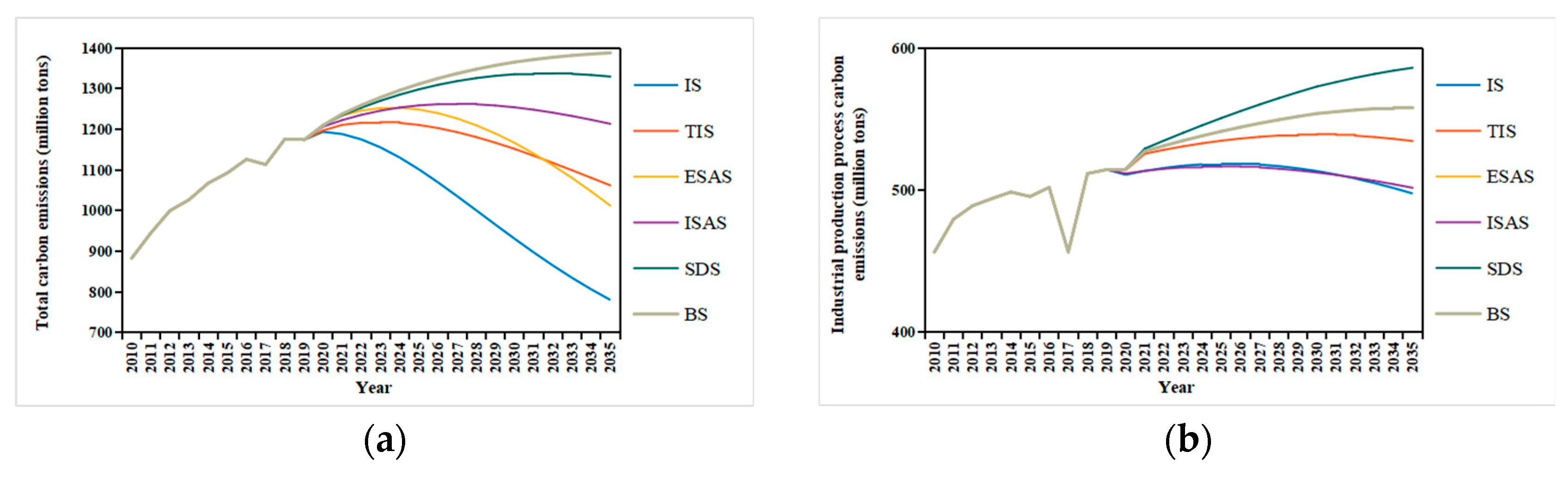
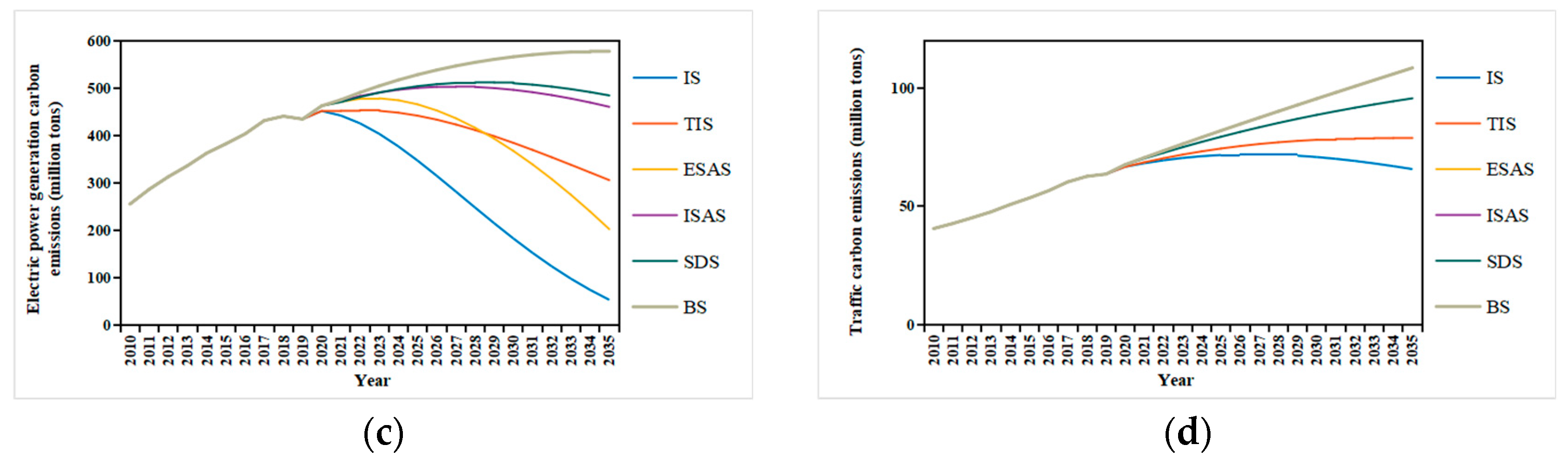
By implementing emission reduction policies, carbon emissions can be effectively reduced. Among them, integrated policies have the best emission reduction effect. Compared with no implementation of any policies, by 2035, integrated policies can reduce CO2 emissions by 43.68%. Adjusting the energy structure has the best emission reduction effect among the four single-policy scenarios (SDS, ISAS, ESAS, and TIS). Compared with no implementation of any policies, this policy can reduce CO2 emissions by 27.22%.
(3)
By implementing emission reduction policies, carbon peak time can be reached much earlier. Except for economic and social development policies, the implementation of other policies can achieve carbon peak targets by 2030. Among them, integrated policies can achieve carbon peak targets as early as possible, and the carbon peak amount is the lowest. Among the four single-policy scenarios (SDS, ISAS, ESAS, and TIS), increasing investment in technological innovation is the best strategy to reach carbon peak targets at the earliest.
(4)
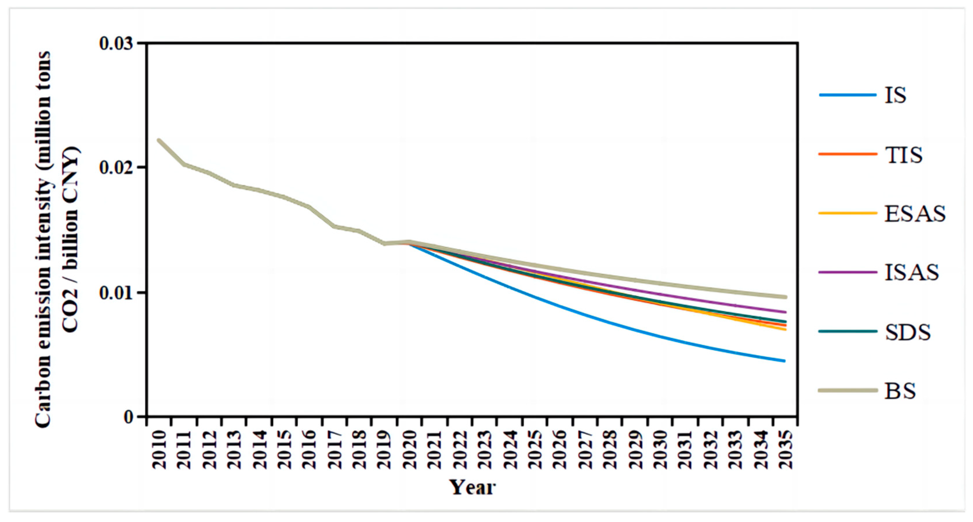
The carbon emission intensity of the BTHUA maintained a slow downward trend from 2010 to 2019. Based on current policies (i.e., the BS), it is predicted in this study that the carbon emission intensity will continue to decline in the future. By implementing emission reduction policies, we can further reduce the carbon emission intensity and promote a comprehensive green and low-carbon transformation of the economy and society. Compared with not implementing any policies, integrated policies can reduce carbon emission intensity by 53.26% by 2035. Adjusting the energy structure has the best effect among the four single-policy scenarios (SDS, ISAS, ESAS, and TIS). Compared with not implementing any policies, this policy can reduce CO2 emissions intensity by 27.05%.
(5)
For various evaluation indicators, integrated policies always have the best effect. However, from the simulation data, the evidence shows that the carbon reduction effects of integrated policies are not a simple summation of the emission reduction effects of other single-policy measures. In addition, the simultaneous implementation of multiple policy measures also means investing more human resources, material resources, and financial resources. Therefore, policies should be scientifically and reasonably formulated and implemented under local conditions, and policies should not be blindly added in pursuit of low CO2 emissions. This paper provides the optimal emission reduction measures based on different emission reduction indicators, providing some suggestions and support for policy formulation.
Based on the research findings, the policy implications are as follows: (1) The current industrial structure and energy structure of the BTHUA cannot ensure that the peak carbon target can be realized, and the economy is developing at a high speed. Therefore, it is more suitable for the current development needs of the BTHUA to shift from high-speed development to high-quality development, and to decouple economic growth from carbon emissions as soon as possible. (2) Given that industrial production is the most important driver of carbon emissions in the BTHUA, accelerating the green transformation of the industry and promoting the transformation of the entire industrial structure toward cleaner, more energy-saving, and more efficient production is the key measure to realize the goal of carbon peak. (3) Integrated policies always work best. The key to achieving the carbon peak target is to integrate different measures, such as improving energy efficiency, adjusting the energy structure, increasing the number of carbon sinks, guiding the behavior of residents, and optimizing the industrial structure. Of course, this implies many times the current investment and efforts.
This study explores the impacts of four single-policy scenarios and integrated-policy scenarios on carbon emission reduction in urban agglomerations. It was found that the implementation of different policies generates different costs, and the implementation of integrated policies implies the generation of more costs. However, how to quantify these costs scientifically was not considered in detail in this study. In further research, we will conduct a more in-depth study on the costs of implementing these policies and improve the recommendations by providing more precise emission reduction suggestions for policymakers from the perspectives of both the costs of policy implementation and the emission reduction benefits generated by the policies.

Author Contributions

Conceptualization, Y.Z. and J.W.; methodology, W.Z. and L.S.; data curation, W.Z. and J.S.; validation, W.Z. and L.S.; writing—original draft preparation, W.Z.; writing—review and editing, Y.Z. and J.W. All authors have read and agreed to the published version of the manuscript.

Funding

This research was funded by the National Key Research and Development Program, grant number 2016YFF020440502; the Foreign Expert’s Program of the Ministry of Science and Technology of China, grant number G2022106001L; and the Funds for First-class Discipline Construction, grant number XK1802-5.

Data Availability Statement

Not applicable.

Conflicts of Interest

The authors declare no conflict of interest.

Appendix A

Table A1. Equations of the SD model.
EquationUnit
Afforestation investment = 0.0287641 × GDP − 672.059Billion CNY
Bus = INTEG (Bus incremental value, 46,054)Vehicle Unit
Bus incremental value = 15.5799 × Investment in transport infrastructure − 6512.35Vehicle Unit
BUSCE = Bus × BUSCECMillion Tons
BUSCEC = 1.99386 × 10⁻⁴ × EXP ((−2.04312 × 10⁻⁴) × Technology investment)-
Car = INTEG (Car incremental value, 9.2874 × 10⁶)Vehicle Unit
Car incremental value = 1.98481 × Per Capita GDP + 1.38588 × 10⁶Vehicle Unit
Carbon intensity = Total carbon emissions/GDPMillion tons/Billion CNY
Carbon sink = Forest carbon sink + Grassland carbon sink + Ocean carbon sequestration fluxMillion Tons
CARCE = CARCEC × CarMillion Tons
CARCEC = 1.46597 × 10⁻⁶ × EXP((−1.96062 × 10⁻⁴) × Technology investment)-
DCE = Residential energy consumption × DCECMillion Tons
DCEC = 0.0169-
Energy consumption in industrial production processes = 0.245 × Industrial production output value + 0.764 × Energy consumption in the secondary industry104 × Tce
Energy consumption in the secondary industry = 6851.73 × LN(Output value of the secondary industry) − 36,319.7104 × Tce
Forest area incremental value = 7.22399 × 10⁻³ × Afforestation investment − 1.47019104 × Hectare
Forest carbon sequestration factor = 1.6-
Forest carbon sink = Forest carbon sequestration factor × Total forest areaMillion Tons
Fossil energy generation = 10,527 × ICOFEPG − 3.59253 × 10⁷KW
GDP = INTEG (GDP incremental value, 39,798.40)Billion CNY
GDP growth rate = WITH LOOKUP (Time, ([(0, 0) − (3000, 10)], (2010, 0.173064), (2011, 0.0955149), (2012, 0.082012), (2013, 0.062087), (2014, 0.0558291), (2015, 0.0795332), (2016, 0.0892899), (2017, 0.0820749), (2018, 0.069849), (2019, 0.0198739), (2020, 0.0515417), (2021, 0.0485604), (2022, 0.0457515), (2023, 0.0431052), (2024, 0.0406118), (2025, 0.0382627), (2026, 0.0360495), (2027, 0.0339643), (2028, 0.0319997), (2029, 0.0301488), (2030, 0.0284049), (2031, 0.0267619), (2032, 0.0252139), (2033, 0.0237555), (2034, 0.0223814), (2035, 0.0210868)))-
GDP incremental value = GDP × GDP growth rateBillion CNY
Grassland area = 0.552534104 × Hectare
Grassland carbon sequestration factor = 1.3-
Grassland carbon sink = Grassland carbon sequestration factor × Grassland areaMillion Tons
ICFFEPGIV = IF THEN ELSE (Time <= 2015, 280, 0.140532 × Proportion of fossil fuels × Energy consumption in the secondary industry − 3561.93)104 × Tce
ICFNFEPGIV = IF THEN ELSE (Time <= 2015, 330, 0.702402 × Energy consumption in the secondary industry × “Proportion of non-fossil fuels” − 2880.87)104 × Tce
ICOFEPG = INTEG (ICFFEPGIV, 4918)KW
ICONFEPG = INTEG (ICFNFEPGIV, 0)KW
Industrial production output value = Output value of the secondary industry × Proportion of industrial production output valueBillion CNY
Investment in transport infrastructure = 709.837 × LN(GDP) − 7123.11Billion CNY
IPPCE = IF THEN ELSE (Time = 2017, 45,642.2, IPPCEC × Energy consumption in industrial production processes)Million Tons
IPPCEC = 1.80874 × 10⁻² × EXP ((−1.67338 × 10⁻⁵) × Technology investment)-
Net carbon emissions = Total carbon emissions − carbon sinkMillion Tons
NEVCE = New energy vehicles × NEVCECMillion Tons
NEVCEC = 9.48802 × 10⁻⁵ × EXP ((−1.17821 × 10⁻⁴) × Technology investment)-
New energy vehicles = INTEG (New energy vehicles incremental value, 43,299)Vehicle Unit
New energy vehicles incremental value = 4.57677 × Technology investment + 227.423Billion CNY
OCE = WITH LOOKUP (Time, ([(2010, 0) − (2035, 7000)], (2010, 6046),(2011, 5871), (2012, 6793.14), (2013, 5708.13), (2014, 5732.44), (2015, 5895.85), (2016, 5817.77), (2017, 5564.29), (2018, 4822.63), (2019, 4654.11), (2020, 4839.97), (2021, 4685.32), (2022, 4530.67), (2023, 4376.02), (2024, 4221.38), (2025, 4066.73), (2026, 3912.08), (2027, 3757.43), (2028, 3602.78), (2029, 3448.13), (2030, 3293.49), (2031, 3138.84), (2032, 2984.19), (2033, 2829.54), (2034, 2674.89), (2035, 2520.24)))-
Ocean carbon sequestration flux = 8.55-
Output value of the secondary industry = GDP × Proportion of secondary industryBillion CNY
Per Capita GDP = GDP/Total populationBillion CNY/104
PGCE = Fossil energy generation × PGCECMillion Tons
PGCEC = 2.16474 × 10⁻⁵ × EXP ((−2.44594 × 10⁻⁴) × Technology investment)-
Population growth rate = WITH LOOKUP (Time, ([(2010, −0.0009) − (2030, 0.03282)], (2010, 0.0152), (2011, 0.01473), (2012, 0.01389), (2013, 0.01214), (2014, 0.00816), (2015, 0.00763158), (2016, 0.00608), (2017, 0.00535), (2018, 0.0043), (2019, 0.00312), (2020, 0.00266), (2021, 0.001538), (2022, 0.00086), (2023, 0.000292), (2024, −0.00016), (2025, −0.00051), (2026, −0.00075), (2027, −0.00087), (2028, −0.00089), (2029, −0.00079), (2030, −0.00059), (2031, −0.00027), (2032, 0.000155), (2033, 0.000692), (2034, 0.00134), (2035, 0.002098)))-
Population incremental value = Total population × Population growth rate104
Proportion of fossil fuels = 1 − “Proportion of non-fossil fuels”-
Proportion of industrial production output value = WITH LOOKUP (Time, ([(0, 0) − (3000, 10)], (2010, 0.86477), (2011, 0.865141), (2012, 0.863427), (2013, 0.860274), (2014, 0.854771), (2015, 0.846436), (2016, 0.849644), (2017, 0.840986), (2018, 0.832658), (2019, 0.837231), (2020, 0.830611), (2021, 0.826807), (2022, 0.823003), (2023, 0.819199), (2024, 0.815395), (2025, 0.811591), (2026, 0.807786), (2027, 0.803982), (2028, 0.800178),(2029, 0.796374), (2030, 0.79257), (2031, 0.788766), (2032, 0.784962), (2033, 0.781158), (2034, 0.777353), (2035, 0.773549)))-
“Proportion of non-fossil fuels” = WITH LOOKUP (Time, ([(2010, 0) − (2035, 1)], (2010, 0.111849), (2011, 0.119596), (2012, 0.119371), (2013, 0.139841), (2014, 0.138108), (2015, 0.133127), (2016, 0.142367), (2017, 0.149612), (2018, 0.14858), (2019, 0.153829), (2020, 0.160112), (2021, 0.164563), (2022, 0.169015), (2023, 0.173466), (2024, 0.177918), (2025, 0.182369), (2026, 0.186821), (2027, 0.191272), (2028, 0.195724), (2029, 0.200175), (2030, 0.204627), (2031, 0.209079), (2032, 0.21353), (2033, 0.217982), (2034, 0.222433), (2035, 0.226885)))-
Proportion of secondary industry = WITH LOOKUP (Time, ([(2010, 0) − (2060, 0.4)], (2010, 0.37598), (2011, 0.37688), (2012, 0.369726), (2013, 0.356855), (2014, 0.349216), (2015, 0.329196), (2016, 0.318932), (2017, 0.30684), (2018, 0.294019), (2019, 0.284191), (2020, 0.281437), (2021, 0.29024), (2022, 0.285663), (2023, 0.281515), (2024, 0.27773), (2025, 0.274251), (2026, 0.271036), (2027, 0.26805), (2028, 0.265266), (2029, 0.262658), (2030, 0.260208), (2031, 0.257098), (2032, 0.254294), (2033, 0.251491), (2034, 0.248687), (2035, 0.245883)))-
Rail transit = INTEG (Rail transit incremental value, 2755)Vehicle Unit
Rail transit incremental value = 1.40466 × Investment in transport infrastructure − 275.37Billion CNY
Residential energy consumption = 2.8062 × Total population − 25,203.9104 × Tce
RTCE = Rail transit × RTCECMillion Tons
RTCEC = 889,396 ×10−4 × EXP ((−1.9907910−4) × Technology investment)-
Taxi = INTEG (Taxi incremental value, 144,602)Vehicle Unit
Taxi incremental value = 0.782137 × Investment in transport infrastructure + 1050.85Billion CNY
TAXICE = Taxi × TAXICECMillion Tons
TAXICEC = 0.0000501074 × EXP((−3.06312 × 10⁻⁵) × Technology investment)-
TCE = BUSCE + TAXICE + TRUCKCE + NEVCE + CARCE + RTCEMillion Tons
Technology investment = GDP × Technology investment ratioBillion CNY
Technology investment ratio = WITH LOOKUP (Time, ([(2010, 0) − (2035, 0.05)], (2010, 0.0303237), (2011, 0.0307531), (2012, 0.0326447), (2013, 0.034255), (2014, 0.0348397), (2015, 0.0361981), (2016, 0.0359043), (2017, 0.0341271), (2018, 0.0347138), (2019, 0.037221), (2020, 0.0372676), (2021, 0.0373141), (2022, 0.0373607), (2023, 0.0374072), (2024, 0.0374538), (2025, 0.0375003), (2026, 0.0375469), (2027, 0.0375935), (2028, 0.03764), (2029, 0.0376866), (2030, 0.0377331), (2031, 0.0377797), (2032, 0.0378262), (2033, 0.0378728), (2034, 0.0379193), (2035, 0.0379659)))-
Total carbon emissions = TCE + OCE + PGCE + IPPCE+ DCEMillion Tons
Total forest area = INTEG (Forest area incremental value, 483.96)104 × Hectare
Total population = INTEG (Population incremental value, 10,454.8)104
Truck = INTEG (Truck incremental value, 1.6004 × 10⁶)Vehicle Unit
Truck incremental value = 0.651127 × GDP + 164,883Billion CNY
TRUCKCE = Truck × TRUCKCECMillion Tons
TRUCKCEC = 7.15537 ×10⁻⁶ × EXP ((−9.50746 × 10⁻⁵) × Technology investment)-

References

  1. IPCC. The Ocean and Cryosphere in a Changing Climate; Cambridge University Press: Cambridge, UK; New York, NY, USA, 2022. [Google Scholar]
  2. Thackeray, S.J.; Robinson, S.A.; Smith, P.; Bruno, R.; Kirschbaum, M.U.F.; Bernacchi, C.; Byrne, M.; Cheung, W.; Cotrufo, M.F.; Gienapp, P.; et al. Civil disobedience movements such as School Strike for the Climate are raising public awareness of the climate change emergency. Glob. Chang. Biol. 2020, 26, 1042–1044. [Google Scholar] [CrossRef] [PubMed]
  3. IPCC. Climate Change 2022: Impacts, Adaptation and Vulnerability; Cambridge University Press: Cambridge, UK; New York, NY, USA, 2022; pp. 121–196. [Google Scholar]
  4. Cai, L.; Luo, J.; Wang, M.; Guo, J.; Duan, J.; Li, J.; Li, S.; Liu, L.; Ren, D. Pathways for municipalities to achieve carbon emission peak and carbon neutrality: A study based on the LEAP model. Energy 2023, 262, 125435. [Google Scholar] [CrossRef]
  5. Li, R.; Yu, Y.H.; Cai, W.G.; Liu, Q.Q.; Liu, Y.; Zhou, H.A. Interprovincial differences in the historical peak situation of building carbon emissions in China: Causes and enlightenments. J. Environ. Manag. 2023, 332, 117347. [Google Scholar] [CrossRef] [PubMed]
  6. Le Quéré, C.; Korsbakken, J.I.; Wilson, C.; Tosun, J.; Andrew, R.; Andres, R.J.; Canadell, J.G.; Jordan, A.; Peters, G.P.; van Vuuren, D.P. Drivers of declining CO2 emissions in 18 developed economies. Nat. Clim. Chang. 2019, 9, 213–217. [Google Scholar] [CrossRef]
  7. El Anshasy, A.A.; Katsaiti, M.S. Energy intensity and the energy mix: What works for the environment? J. Environ. Manag. 2014, 136, 85–93. [Google Scholar] [CrossRef]
  8. Erdoğan, S.; Yıldırım, S.; Yıldırım, D.Ç.; Gedikli, A. The effects of innovation on sectoral carbon emissions: Evidence from G20 countries. J. Environ. Manag. 2020, 267, 110637. [Google Scholar] [CrossRef] [PubMed]
  9. Papadis, E.; Tsatsaronis, G. Challenges in the decarbonization of the energy sector. Energy 2020, 205, 118025. [Google Scholar] [CrossRef]
  10. Bruninx, K.; Ovaere, M. COVID–19, Green Deal and recovery plan permanently change emissions and prices in EU ETS Phase IV. Nat. Commun. 2022, 13, 1165. [Google Scholar] [CrossRef]
  11. Green, J.F. Does carbon pricing reduce emissions? A review of ex-post analyses. Environ. Res. Lett. 2021, 16, 043004. [Google Scholar] [CrossRef]
  12. Stainforth, D.A. ‘Polluter pays’ policy could speed up emission reductions and removal of atmospheric CO2. Nature 2021, 596, 346–347. [Google Scholar] [CrossRef]
  13. Wang, H.G.; Xiao, L.X.; Liao, B. Simulation of China’s carbon emission reduction path based on system dynamics. J. Nat. Resour. 2022, 37, 1352–1369. [Google Scholar] [CrossRef]
  14. Trail, M.A.; Tsimpidi, A.P.; Liu, P.; Tsigaridis, K.; Hu, Y.T.; Rudokas, J.R.; Miller, P.J.; Nenes, A.; Russell, A.G. Impacts of potential CO2–reduction policies on air quality in the United States. Environ. Sci. Technol. 2015, 49, 5133–5141. [Google Scholar] [CrossRef] [PubMed]
  15. Wang, Q.; Wang, X.W.; Li, R.R. Does urbanization redefine the environmental Kuznets curve? An empirical analysis of 134 Countries. Sustain. Cities Soc. 2022, 76, 103382. [Google Scholar] [CrossRef]
  16. Wang, Q.; Sun, J.; Pata, U.K.; Li, R.R.; Kartal, M.T. Digital economy and carbon dioxide emissions: Examining the role of threshold variables. Geosci. Front. 2023, 101644. [Google Scholar] [CrossRef]
  17. Li, R.R.; Wang, Q.; Liu, Y.; Jiang, R. Per-capita carbon emissions in 147 countries: The effect of economic, energy, social, and trade structural changes. Sustain. Prod. Consum. 2021, 27, 1149–1164. [Google Scholar] [CrossRef]
  18. Wang, Q.; Zhang, F.Y.; Li, R.R. Revisiting the environmental kuznets curve hypothesis in 208 counties: The roles of trade openness, human capital, renewable energy and natural resource rent. Environ. Res. 2023, 216, 114637. [Google Scholar] [CrossRef] [PubMed]
  19. Wang, Q.; Wang, L.L.; Li, R.R. Trade openness helps move towards carbon neutrality—Insight from 114 countries. Sustain. Dev. 2023. [Google Scholar] [CrossRef]
  20. Wang, Q.; Zhang, F.Y.; Li, R.R. Free trade and carbon emissions revisited: The asymmetric impacts of trade diversification and trade openness. Sustain. Dev. 2023. [Google Scholar] [CrossRef]
  21. Xiang, N.; Xu, F. Optimization path simulation of carbon emission peak in Beijing–based on structure and efficiency improvement. J. Beijing Univ. Technol. (Soc. Sci. Ed.) 2022, 22, 68–87. [Google Scholar]
  22. Wang, Y.; Bi, Y.; Wang, E.D. Scene prediction of carbon emission peak and emission reduction potential estimation in Chinese industry. China Popul. Resour. Environ. 2017, 27, 131–140. [Google Scholar]
  23. Ofori, E.K.; Li, J.; Gyamfi, B.A.; Opoku-Mensah, E.; Zhang, J. Green industrial transition: Leveraging environmental innovation and environmental tax to achieve carbon neutrality. Expanding on STRIPAT model. J. Environ. Manag. 2023, 343, 118121. [Google Scholar] [CrossRef] [PubMed]
  24. Handayani, K.; Anugrah, P.; Goembira, F.; Overland, I.; Suryadi, B.; Swandaru, A. Moving beyond the NDCs: ASEAN pathways to a net–zero emissions power sector in 2050. Appl. Energy 2022, 311, 118580. [Google Scholar] [CrossRef]
  25. Mirzaei, M.; Bekri, M. Energy consumption and CO2 emissions in Iran, 2025. Environ. Res. 2017, 154, 345–351. [Google Scholar] [CrossRef]
  26. Xu, N.; Ding, S.; Gong, Y.D.; Bai, J. Forecasting Chinese greenhouse gas emissions from energy consumption using a novel grey rolling model. Energy 2019, 175, 218–227. [Google Scholar] [CrossRef]
  27. Chen, X.; Shuai, C.; Wu, Y.; Zhang, Y. Analysis on the carbon emission peaks of China’s industrial, building, transport, and agricultural sectors. Sci. Total Environ. 2019, 709, 135768. [Google Scholar] [CrossRef] [PubMed]
  28. Gao, G.L.; Wen, Y.; Wang, L.; Xu, R.N. Study on carbon peak of urban clusters based on analysis of influencing factors of carbon emissions. Bus. Manag. J. 2023, 45, 39–58. [Google Scholar]
  29. Fang, G.C.; Tian, L.X.; Fu, M.; Sun, M.; Du, R.J.; Liu, M.H. Investigating carbon tax pilot in YRD urban agglomerations–Analysis of a novel ESER system with carbon tax constraints and its application. Appl. Energy 2017, 194, 635–647. [Google Scholar] [CrossRef]
  30. Zhang, Z.F.; Zhang, D. Spatial relatedness of CO2 emission and carbon balance zoning in Beijing Tianjin Hebei counties. China Environ. Sci. 2023, 43, 2057–2068. [Google Scholar]
  31. Lian, J.H.; Lauvaux, T.; Utard, H.; Breon, F.M.; Broquet, G.; Ramonet, M.; Laurent, O.; Albarus, I.; Cucchi, K.; Ciais, P. Assessing the effectiveness of an urban CO2 monitoring network over the Paris region through the COVID–19 lockdown natural experiment. Environ. Sci. Technol. 2022, 56, 2153–2162. [Google Scholar] [CrossRef]
  32. Wang, C.; Zhan, J.Y.; Bai, Y.P.; Chu, X.; Zhang, F. Measuring carbon emission performance of industrial sectors in the Beijing–Tianjin–Hebei region, China: A stochastic frontier approach. Sci. Total Environ. 2019, 685, 786–794. [Google Scholar] [CrossRef]
  33. Qudrat–Ullah, H.; Seong, B.S. How to do structural validity of a system dynamics type simulation model: The case of an energy policy model. Energy Policy 2010, 38, 2216–2224. [Google Scholar] [CrossRef]
  34. Xiao, S.J.; Dong, H.J.; Geng, Y.; Tian, X. Low carbon potential of urban symbiosis under different municipal solid waste sorting modes based on a system dynamic method. Resour. Conserv. Recycl. 2022, 179, 106108. [Google Scholar] [CrossRef]
  35. Sim, J.; Sim, J. The effect of new carbon emission reduction targets on an apartment building in South Korea. Energy Build. 2016, 127, 637–647. [Google Scholar] [CrossRef]
  36. Roberts, S.H.; Foran, B.D.; Axon, C.J.; Warr, B.S.; Goddard, N.H. Consequences of selecting technology pathways on cumulative carbon dioxide emissions for the United Kingdom. Appl. Energy 2018, 228, 409–425. [Google Scholar] [CrossRef]
  37. Wang, Y.J.; Lin, X. A review of climate change and its impact and adaptation in Beijing-Tianjin-Hebei urban agglomeration. Clim. Chang. Res. 2022, 18, 743–755. [Google Scholar]
  38. Wang, Z.B.; Liang, L.W.; Sun, Z.; Wang, X.M. Spatiotemporal differentiation and the factors influencing urbanization and ecological environment synergistic effects within the Beijing-Tianjin-Hebei urban agglomeration. J. Environ. Manag. 2019, 243, 227–239. [Google Scholar] [CrossRef]
  39. Yan, X.H.; Gao, D.; Li, Y. Thoughts and Countermeasures on Promoting Energy Revolution in the Beijing–Tianjin–Hebei Region. Engineering 2021, 23, 24–31. [Google Scholar] [CrossRef]
  40. Fankhauser, S.; Smith, S.M.; Allen, M.; Axelsson, K.; Hale, T.; Hepburn, C.; Kendall, J.M.; Khosla, R.; Lezaun, J.; Mitchell-Larson, E.; et al. The meaning of net zero and how to get it right. Nat. Clim. Chang. 2022, 12, 15–21. [Google Scholar] [CrossRef]
  41. Mostafaeipour, A.; Bidokhti, A.; Fakhrzad, M.B.; Sadegheih, A.; Mehrjerdi, Y.Z. A new model for the use of renewable electricity to reduce carbon dioxide emissions. Energy 2022, 238, 121602. [Google Scholar] [CrossRef]
  42. Yang, H.H.; Li, X.; Ma, L.W.; Li, Z. Using system dynamics to analyse key factors influencing China’s energy-related CO2 emissions and emission reduction scenarios. J. Clean. Prod. 2021, 320, 128811. [Google Scholar] [CrossRef]
  43. Bernardo, G.; D’Alessandro, S. Systems–dynamic analysis of employment and inequality impacts of low–carbon investments. Environ. Innov. Soc. Transit. 2016, 21, 123–144. [Google Scholar] [CrossRef]
  44. Li, W.; An, C.L.; Lu, C. The assessment framework of provincial carbon emission driving factors: An empirical analysis of Hebei Province. Sci. Total Environ. 2018, 637, 91–103. [Google Scholar] [CrossRef] [PubMed]
  45. Dai, T.J.; An, B.C.; Wang, W.J. Path analysis of coordinated development of resource, environment and economy in Beijing–Tianjing–Hebei region. J. Ecol. Rural Environ. 2020, 36, 731–740. [Google Scholar]
  46. Yang, Y.; He, F.; Ji, J.P.; Liu, X. Peaking carbon emissions in a megacity through economic restructuring: A case study of Shenzhen, China. Energies 2022, 15, 6932. [Google Scholar] [CrossRef]
  47. Liu, Y.R.; Tang, L.; Liu, G.F. Carbon dioxide emissions reduction through technological innovation: Empirical evidence from Chinese provinces. Int. J. Environ. Res. Public Health 2022, 19, 9543. [Google Scholar] [CrossRef]
  48. Jia, P.R.; Li, K.; Shao, S. Choice of technological change for China’s low-carbon development: Evidence from three urban agglomerations. J. Environ. Manag. 2018, 206, 1308–1319. [Google Scholar] [CrossRef]
  49. Qin, H.T.; Huang, Q.H.; Zhang, Z.W.; Lu, Y.; Li, M.C.; Xu, L.; Chen, Z.J. Carbon dioxide emission driving factors analysis and policy implications of Chinese cities: Combining geographically weighted regression with two-step cluster. Sci. Total Environ. 2019, 684, 413–424. [Google Scholar] [CrossRef]
  50. Gu, R.D.; Li, C.F.; Li, D.D.; Yang, Y.Y.; Gu, S. The impact of rationalization and upgrading of industrial structure on carbon emissions in the Beijing-Tianjin-Hebei urban agglomeration. Int. J. Environ. Res. Public Health 2022, 19, 7997. [Google Scholar] [CrossRef]
  51. Wang, J.; Feng, L.; Palmer, P.I.; Liu, Y.; Fang, S.X.; Bosch, H.; O’Dell, C.W.; Tang, X.; Yang, D.; Liu, L.; et al. Large Chinese land carbon sink estimated from atmospheric carbon dioxide data. Nature 2020, 586, 720–723. [Google Scholar] [CrossRef] [PubMed]
Figure 1. Carbon emissions in the BTHUA.
Energies 16 06654 g001
Figure 2. Causal loop diagram of the BTHUA’s carbon emission.
Energies 16 06654 g002
Figure 3. Mechanism of emission reduction policies.
Energies 16 06654 g003
Figure 4. The SD model of the BTHUA’s carbon emissions.
Energies 16 06654 g004
Figure 5. The sensitivity analysis results (unit: million tons).
Energies 16 06654 g005
Figure 6. Carbon emissions in different scenarios (unit: million tons): (a) total carbon emissions; (b) industrial production process carbon emissions; (c) power generation carbon emissions; (d) traffic carbon emissions.
Energies 16 06654 g006aEnergies 16 06654 g006b
Figure 7. Net carbon emissions in different scenarios (unit: million tons).
Energies 16 06654 g007
Figure 8. Carbon emission intensity in different scenarios (unit: million tons CO2/billion CNY).
Energies 16 06654 g008
Table 1. Validity assessment of the SD model.
Variable 2010201120122013201420152016201720182019
GDP (1010 CNY)Historical value398.0466.9511.5553.4587.8620.6669.9729.7789.6844.8
Simulation value398.0466.9511.5553.4587.8620.6669.9729.8789.6844.8
Relative error (%)0.000.000.000.000.000.000.000.000.000.00
Total population (104)Historical value104.6106.2107.7109.2110.5111.4112.1112.5112.7110.2
Simulation value104.6106.1107.7109.2110.5111.4112.3113.0113.6114.1
Relative error (%)0.00−0.010.000.00−0.01−0.010.200.420.763.47
Total carbon emissions (million tons)Historical value926.01010.31010.11076.81042.81035.51046.51021.91155.01160.8
Simulation value882.7944.7999.71026.81067.51092.61126.21113.21175.41173.7
Relative error (%)−4.68−6.50−1.03−4.652.365.517.628.941.771.11
Table 2. Scenarios and key variables settings of sensitivity analysis.
ScenarioDescription
BS-
S1GDP growth rate + 10%
S2Population growth rate + 10%
S3Proportion of secondary industry − 10%
S4Proportion of non-fossil fuels + 10%
S5Technology investment ratio + 10%
Table 3. Scenarios and key variable settings.
ScenarioDescription
BSDevelop according to current policies.
SDSThis scenario simulates the situation of economic and population growth. We increased the GDP growth rate to 6.40% in 2020 and slowly decreased it to 3.30% in 2035. Meanwhile, considering the fact that the population growth rate of the BTHUA has been continuously decreasing in recent years, we set the population growth rate from 2020 to 2035 to remain unchanged based on the population growth rate of 0.27% in 2020. The remaining variables were consistent with the BS.
ISASThis scenario simulates the optimization of industrial structure. We decreased the proportion of the secondary industry to 18.00% in 2035. The remaining variables were consistent with the BS.
ESASThis scenario simulates the adjustment of the energy structure. We increased the proportion of non-fossil fuels to 40.00% in 2035. The remaining variables were consistent with the BS.
TISThis scenario simulates the progress of technology. We increased the proportion of technology investment to 5.60% in 2035. The remaining variables were consistent with the BS.
ISThis scenario contains all the controls for SDS, ISAS, ESAS, and TIS, with the remaining variable settings consistent with the BS.
Disclaimer/Publisher’s Note: The statements, opinions and data contained in all publications are solely those of the individual author(s) and contributor(s) and not of MDPI and/or the editor(s). MDPI and/or the editor(s) disclaim responsibility for any injury to people or property resulting from any ideas, methods, instructions or products referred to in the content.

