Abstract
In single phase flows, benchmarks like the lid driven cavity have become recognized as fundamental tests for newly developed computational fluid dynamics, CFD, codes. For multiphase free surface flows with variable surface tension, the presently studied pool with isothermal sidewalls is suggested as it is the simplest domain where Marangoni effects can dominate. It was also chosen due to its strange sensitivity to the initial setup which is discussed at length from a chosen number of ‘scenarios’. It was found that the fluid interface can reverse deformation by a change in the top boundary condition, the liquid equation of state, and the gravity level. For the top boundary condition, this reversal is due to vapor expansion within the closed volume, creating an additional convection mechanism. Not only does the interface reverse, but the peak height changes by more than an order of magnitude at the same Marangoni number. When including gravity, the peak velocity can increase significantly, but it can also cause a decrease when done in combination with a change in the top wall boundary condition. Finally, thermal expansion of the liquid phase causes the peak velocity to be reduced, with additional reductions from the gravity and top wall condition. The differences in each scenario could lead to significant errors in analyzing a practical application of Marangoni flows. Therefore, it is important to demonstrate that a new CFD code can not only resolve Marangoni convection, but also has the capability to resolve the scenario most relevant to the application at hand.
1. Introduction
Surface tension arises from the balance of intermolecular interactions at the interface between phases. Perpendicular to the interface, molecules can adjust their distance towards the minimum interaction potential and creates the interface with a small thickness. In the parallel direction, the molecules are constrained by symmetry and cannot adjust their distance, leading to an excess energy at the interface. Introducing a temperature or species gradient modifies the potential locally resulting in a force imbalance tangential to the interface, and thus an acceleration. These gradients create what is called Marangoni convection, and fluid will move from areas of lower surface tension to areas of higher surface tension. In most fluids, the change in surface tension with temperature, , is nearly linear and negative. As a result, a local increase in temperature gives a decrease in the local surface tension coefficient, . The areas of low surface tension “hold together” less strongly and thus the fluid “expands” towards areas of higher surface tension. Whereas the areas of higher surface tension “pull in” fluid from elsewhere.
Marangoni convection must therefore be considered or even exploited across many heat transfer applications where surface tension is dominant. These include many industrial processes such as drying of integrated circuits [1]; welding processes [2], crystal growth [3], and additive manufacturing [4]. Another common application of the Marangoni effect is in small scale heat transfer devices such as heat pipes which are used ubiquitously across many industries [5]. Within heat pipes, the liquid phase clings to the walls, while a vapor core exists in the center. For maximum heat transfer, vapor convection should be toward the cold end, and liquid convection away from the cold end. The vapor motion is driven by evaporation at the hot end, which creates a pressure gradient and moves vapor towards the cold end. Condensation then occurs and liquid forms at the cold end, the wick then pulls the condensate back towards the hot end for the cycle to repeat. Due to the temperature gradient, the Marangoni effect opposes the wicking action, and reduces the liquid transport and therefore performance. In some cases the Marangoni effect can dominate over wicking and cause the liquid to stagnate and detach from the wall [6].
Given the importance and wide range of use cases, it is critical for a numerical model to capture this behavior in order to correctly predict the resulting flow. In single phase flows, benchmarks like the lid driven cavity, or back facing step have been well studied and are viewed as fundamental tests for verification and validation of a new CFD code. In multiphase flows with variable surface tension, there is not yet a consistently defined benchmark agreed upon. Often the code is validated directly against a given experimental setup, rather than a generic benchmark.
The objectives of the present work are to, (1) prescribe a generic benchmark for Marangoni convection in CFD codes, (2) demonstrate the impact of a variety of factors on benchmark results and the need for consistency and, (3) develop and validate an open source CFD model for Marangoni convection on a free surface.
The first is completed by choosing the simplest possible setup where Marangoni convection is significant, a shallow liquid pool with constant temperature sidewalls. The second is accomplished by revisiting factors investigated in previous literature that were found to influence the interface deformation from Marangoni convection, as well as additional analysis on factors found to change results significantly. The third goal is accomplished by the development of a variable surface tension model using volume of fluid (VOF) method in openFOAM. Simulation results are validated against the theoretical expressions from Sen and Davis [7], previous CFD results, and the experimental data obtained by Villers and Platten [8]. Additionally, the effects of various factors and boundary conditions on Marangoni convection are isolated and discussed at length.
2. Problem Setup and Existing Work
An idealized benchmark for isolating Marangoni convection is a simple two phase flow in a box, demonstrated by Figure 1. The two-dimensional box contains liquid to a height h, while the rest is vapor. The fluid is placed under a temperature gradient between the two side walls, and the top and bottom walls are insulated.
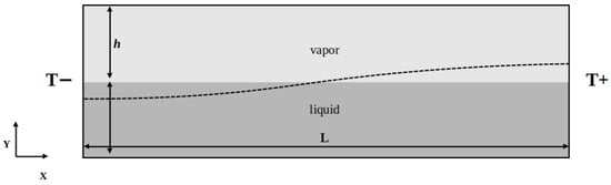
Figure 1.
Fluid domain and thermal boundary conditions. Dashed line shows a representative deformed interface from Maragoni convection.
In this domain, with , fluid at the interface will convect in the negative x direction. The return flow at the cold wall will then create a counterclockwise vortex cell within the liquid phase. The mass flux of these two phenomena (Marangoni convection and the return flow) are equal in steady state, but their velocities are not equal. Marangoni convection occurs only at the thin interface (moving the fluid left), while the return flow occurs throughout the rest of the liquid depth (moving fluid to the right). The profile of the interface will then deform in a possible configuration as shown by the dashed line to reach an equilibrium.
2.1. Literature Review
Marangoni convection has been studied and implemented in openFOAM in a plethora of different applications [9,10,11,12,13,14,15,16]. For brevity the current review is limited to those directly related to the fundamental benchmark of isothermal sidewalls. Many authors have simplified the two-phase problem by neglecting the interface deformation. This is done by creating a wall at and allowing a non-zero velocity at the wall. The tangential surface tension forces are then applied at this boundary. This will be referred to as the single-phase problem. The two-phase problem is then to allow the interface deformation, and also resolve the motion in the vapor phase.
Sen and Davis [7] found an analytical solution for the liquid stream function by asymptotic analysis. Here, the analysis captures the interface deformation and provides an expression based on the capillary number. Shear effects from the vapor phase are neglected, and the interface is taken as thermally insulated. The model assumes an incompressible steady-state single phase flow with an aspect ratio approaching zero.
Bergman and Keller [17] studied the combined effect from buoyancy and Marangoni convection in the single-phase problem. They considered the material properties of liquid aluminum and liquid aluminum-tin alloy, which have negative and positive respectively. The authors found different relations between the Nusselt and Rayleigh numbers when changing , Marangoni number, and domain aspect ratio.
Villers and Platten [8] experimented with Marangoni convection in acetone and studied the velocity profiles and instabilities of the vortices observed. They took multiple velocity profile measurements at and compared the data to CFD results of the single-phase problem. The same authors also developed an analytical model to approximate the velocity profile for an arbitrary value of [18]. This model reduces to that from Sen and Davis [7] for moderate negative values of . The original authors note that the velocity magnitude is not well captured but qualitatively agrees with the profile shape from their experimental results.
Sasmal and Hochstein [19] implemented Marangoni convection using the continuum surface force methodology and investigated the effect of wall contact angle, Marangoni number, and Capillary number in the two-phase problem. The model was benchmarked against an example case from Sen and Davis [7], but the interface shape was not directly compared to the analytical expressions.
Kothe et al. [20] developed an in house multi-physics tool for casting and welding processes which includes a VOF model for multiphase flows, where they used the two-phase problem to benchmark their model. They first studied the single-phase problem and compared the velocity profiles with the analytical stream functions from Bauer and Eidel [21]. The authors then briefly study the two-phase problem and note that the capillary number significantly effects the free surface height at the sidewalls.
Zhou and Huang [22] studied a two-fluid system via the level set method. They found that the interface deformation was reversed to that predicted by the model from Sen and Davis [7] with a large difference in Prandtl number of 9300 to 1. Zhou and Huai [23] later studied the two-phase problem over a range of Marangoni numbers, domain aspect ratio, and gravity levels with a Prandtl ratio of 60 to 1. They found an effect on the interface deformability for each of these parameters. Zhou et al. [24] then considered the effects of species concentration on Marangoni convection in addition to the thermal gradients so far discussed. They studied the effect of Prandtl number, Marangoni number, species concentration, Lewis number, and gravity on the interface deformation. Later, Zhou and Huai [25] studied the ratio between thermal Marangoni and species Marangoni convection. In each of these publications, the main comparison point was the overall interface deformability [23,24,25].
Saldi [26] investigated the complex role of Marangoni convection within melting bismuth under laser welding with a model developed in openFOAM, one of many such works that studied this effect within molten welds. The present review is limited to the work from Saldi, as they used the single-phase and two-phase problems as a fundamental benchmark for their surface tension model. The single-phase results were compared to those from Bergman and Keller [17]. In the two-phase problem, the interface height at either side-wall was compared to previous works, rather than the full profile.
Chen and Xu [27] found various transient regimes in the single-phase problem by analyzing the velocity and time scales of Marangoni convection and viscous effects. The model was validated by comparing the predicted velocity profile with the theory from Sen and Davis [7] and the experimental work from Villers and Platten [8].
Tan et al. [28] experimented with silicone oil and recovered the fluid velocities using PIV, having good agreement with their CFD results. While their geometry and applied heat are significantly different from the isothermal sidewalls setup, their results increase confidence that numerical methods can accurately capture these physics.
Other experimental works on Marangoni flows offer valuable data, but their setups do not align with the isothermal sidewall configuration as in wall configuration in this study. In the works from Kamotani et al. [29] and Montanero et al. [30] meniscus pinning at the sidewalls was exploited to further constrain the liquid phase. Schwabe and Scharmann [31] studied Marangoni convection in an open crucible, but the boundary conditions were quite different from the present work. Additionally, some cases included the crystal melt significantly changing the bottom surface of the pool. These reasons make these works, while valuable and significant contributions to understanding Marangoni convection, not appropriate to compare with results of the two-phase isothermal sidewall problem studied presently.
In summary, more work has been done on the single-phase problem than the free surface two-phase problem. In the study of the two-phase problem, more factors were considered for the interface deformation. With these works, the comparison point is typically the interface deformation and a comparison of the velocity profile isn’t considered. Additionally, most benchmarks compared the interface height at either sidewall and not the overall shape of the interface predicted by Sen and Davis [7].
The present work builds upon the analysis of the two-phase isothermal sidewall problem by conducting a more thorough benchmark and examination of results. From previous literature, an effect has been found for many factors including: Marangoni number, Capillary number, Rayleigh number, domain aspect ratio, and the momentum boundary condition on the top wall. Additionally, there are more advanced combination or ratio effects when including chemical variations [22,23,24,25]. To reduce the number of cases needed to be studied and compared, chemical effects are left for a future study. We investigate the impact of gravity, a range of Marangoni numbers, liquid phase equation of state, vapor phase compressibility, the momentum boundary condition of the top wall, as well as combinations. The selection of these factors is to complete the second objective and demonstrate their impacts on benchmark results.
2.2. Definition of the Flow Problem
Previous work has shown the importance of a benchmark described by consistent nondimensional groups [20]. To fully define problem, the following nondimensional numbers are needed: Rayleigh number Ra, Prandtl number Pr, Marangoni number Ma, and Capillary number Ca. For consistency the set of nondimensional numbers will be defined with an aspect ratio and use a characteristic length of h. Some previous authors defined the aspect ratio inversely or did not include it. The Prandtl number is defined in the usual way,
where is the momentum diffusivity and is the thermal diffusivity. While the capillary number will be defined as
where is the difference in temperature across the domain, and is the nominal surface tension coefficient. In this form it expresses the ratio of tangential surface tension to the normal component, scaled by the aspect ratio. The Rayleigh number is given by
where the expansion coefficient, , is approximated as . This approximation is for the consistency of defining Ra in the various scenarios. For example, if the liquid density is constant, becomes undefined. The Marangoni number is given by
where is the viscosity. While the Reynolds number is found by the relation , but is not required to constrain the problem if Equations (1)–(4) are held constant.
2.3. Boundary and Initial Conditions
In the present work, the flow domain is a two-dimensional box of dimensions as illustrated in Figure 1. The top and bottom walls are insulated, while the left and right are constant temperature. All walls enforce the no slip velocity condition. The liquid phase is initially at a uniform height h. The initial temperature field is a linear fit between the two temperature boundaries. If present, gravity acts in the negative y direction. When the domain is referred to as “open” this means a symmetry plane was used on the top wall boundary. This allows a velocity component normal to the boundary and acts as a von Neumann boundary for all other variables. This was chosen to more closely match the analysis and resulting expression from Sen and Davis [7] who considered the single-phase problem. When the domain is referred to as “closed” the top wall boundary is another non-slip wall.
2.4. Governing Equations
The relevant physics to capture in this type of flow problem are the normal and tangential surface tension, compressibility, buoyancy, viscous forces, heat transfer, and phase interactions. The effects of phase change are not considered in the current model to simplify the validation of the Marangoni convection model. In the present work, the transient form of the governing equations is solved until reaching steady state for added numerical stability. Formulation of the problem can begin from the general conservation equation in differential form based on the continuum assumption,
where is a generic field, is a flux through the control volume, and is a volume potential. Mixture properties are calculated according to
where b is a mixture quantity and is the volume fraction of the phase. This is done for the field density , material properties, as well as the velocity field . Using the mixture quantities allows solving one set of equations for all phases. The downside is that introducing a new field variable requires an additional transport equation for the volume fraction, . However, this is still more computationally efficient than solving two full sets of governing equations in the Eulerian–Eulerian approaches. By letting , and , and expanding the divergence term, the continuity equation is
In general, the compressible form above is used, but for the incompressible cases the above form collapses to . The conservation of momentum is found by letting , and , and given as
where the vector is a volumetric body force, is the identity tensor, and is the viscous stress tensor for a Newtonian fluid. Expanding the divergence and time derivative on the left-hand side of (8) gives
This can be simplified by noting that (7) is present in the second term which must be zero. The final form of the momentum equation is then
At the interface, the effects of interphase slip and drag are not considered. The forces of gravity and surface tension will later be cast into the body force term, .
In either software, STAR-CCM+ [32] or openFOAM [33], the conservation of total energy is solved in terms of temperature. This is found from, , and . The quantity is the total energy, H is the total enthalpy, is the surface heat flux, and is work from pressure. The effects of viscous heating are neglected as the velocities in this problem are small. For the same reason the total enthalpy is approximated as the static enthalpy, making the scalar field, . Substituting ,and into (5), expanding the divergence terms on the left-hand side, and collecting pressure terms gives
Additionally, the specific heat and thermal conductivity are constant and have been taken out of each term. Expanding the divergence term on the left-hand side and dividing through by the specific heat gives
The above form is used by STAR-CCM+ [32] and solved in terms of temperature. The mixture density must be left in this form as it allows the expression to be valid across multiple phases. The term accounts for compression of the interface due to the pressure jump across it. The work from surface tension and gravity forces are accounted in the term. The openFOAM [33] formulation is slightly different, the work from surface tension is included directly in the balance, and work from gravity is neglected. Additionally, the substitution, , is used. The openFOAM formulation is
where is the mean interface curvature. The quantity is proportional to the Laplace pressure, and therefore the term does not need to be included. The other pressure term, , is still included in (13) and can be thought of as the pressure work in the fluid away from the interface. The differences are worth pointing out for completeness, but in practice the two formulations are identical. In Equations (12) and (13), the only appreciable source is the heat diffusion term on the right-hand side, which is identical in both forms. Additionally, the neglecting of work from gravity in the openFOAM formulation will not be significant as the fluid depth parallel to the gravity vector is small.
For a two phase system, the volume fraction continuity is found by letting , and ,
When two phases are present, both CFD programs solve (14) for only the liquid phase, and then ensure mass conservation by satisfying
where N is the total number of phases.
2.5. Surface Tension Model
The commercial CFD code STAR-CCM+ [32] models Marangoni convection by the continuum surface force (CSF) based on the work from [34], but is closed source [35]. Ongoing work by openFOAM developers seeks to expand the multiphase capabilities and have released a framework that includes a model for temperature varying , but does not yet consider any tangential forces [36]. As shown previously by Scriven [37], the normal component of the surface tension force can be found from the familiar
This force component is already implemented in the interFoam family of solvers. The difference now is the surface tension coefficient, , becomes a linear function of temperature,
giving the nominal at the center of the box when . This modification alone is not sufficient to model Marangoni convection, as it still assumes a force balance along the interface. The unit normal, , of the interface is found from the normalized gradient of the volume fraction field,
and the mean surface curvature, , is found from the divergence of the unit normal,
Marangoni convection occurs to due to temperature variations in , which results in a force imbalance that acts along the interface. Therefore, the tangential variation of the temperature field along the interface is needed. This can be found from
where the subscript t denotes the surface tangent direction. The subtraction of the normal direction from the full gradient leaves just the tangential variation. Multiplying by the derivative of the surface tension coefficient with respect to temperature, , gives the tangential force component,
The leading factor of effectively filters the equation to only cells near the interface (i.e., the gradient of the volume fraction is zero away from the interface) and gives units of force per volume. This final form is then included in the body force terms of (10) and (12).
For a case of interest, the nondimensional numbers are chosen, along with reference values of , and a reference pressure . The remaining variables, and , are found by the previous definitions of the nondimensional numbers. The chosen constant parameters are listed in Table 1 in SI units. If there is no gravity, the Rayleigh number becomes zero and the material properties are then taken from the corresponding 1 g case. For most cases, the liquid density is taken as a constant . A few cases linearly varied the liquid density with temperature as

Table 1.
Reference values.
The surface tension coefficient is obtained from (17), and all other material properties are held constant from Table 1. Even though the underlying mechanics that cause viscosity and surface tension are the same, the viscosity is held constant in the present work. In these idealized box flow cases, the temperature gradients are quite moderate and changes in the inertial terms of the governing equations from variation of viscosity would be small.
3. Analytical Model
An analytical solution for the stream function of this problem in the limit of small aspect ratio was found by Sen and Davis [7]. Their solution for the interface height, given below in (24), will be used to compare some numerical results. Here it is presented in terms of physical parameters as
where the subscript ∗ denotes a dimensionless quantity. This can be made dimensional by scaling with the nominal interface height prior to Marangoni convection. Sen and Davis [7] give a confidence range for (24) of . The solutions from Sen and Davis [7] have been used multiple times to model the velocity profile of liquid under Marangoni convection with the below quadratic form,
which shows the overall shape of the profile but not its magnitude. Some previous work simply fits a quadratic profile to their results to show agreement with Sen and Davis [7]. This is insufficient and unnecessary because the magnitude of the velocity profile can be recovered by using the original stream function from Sen and Davis [7].
Starting from Equation (5.3a) from Sen and Davis [7], and substituting their parameter definitions, the stream function in terms of physical parameters is
The variable m is taken as zero corresponding to a 90 contact angle with the side walls [7]. The second term contains Ca, based on (2) which is typically or less and is therefore neglected as it is small compared to the first. Taking the partial derivative with respect to yields a function for the nondimensional velocity in the direction as a function of ,
For the analytical model, the characteristic velocity will be defined as
This velocity scale gives a sense of how dominant Marangoni forces are over the viscous forces. Equation (27) is then scaled with the dimensional ,
which is the dimensional velocity in the x direction as a function of position with an undetermined coefficient, C. However, results show that C should be taken as 2 to capture the magnitude and cancel the units, see Figure 2 and Figure 3. It’s not clear if Equation (5.3a) from Sen and Davis [7] is off by a factor of 2 to account for this.

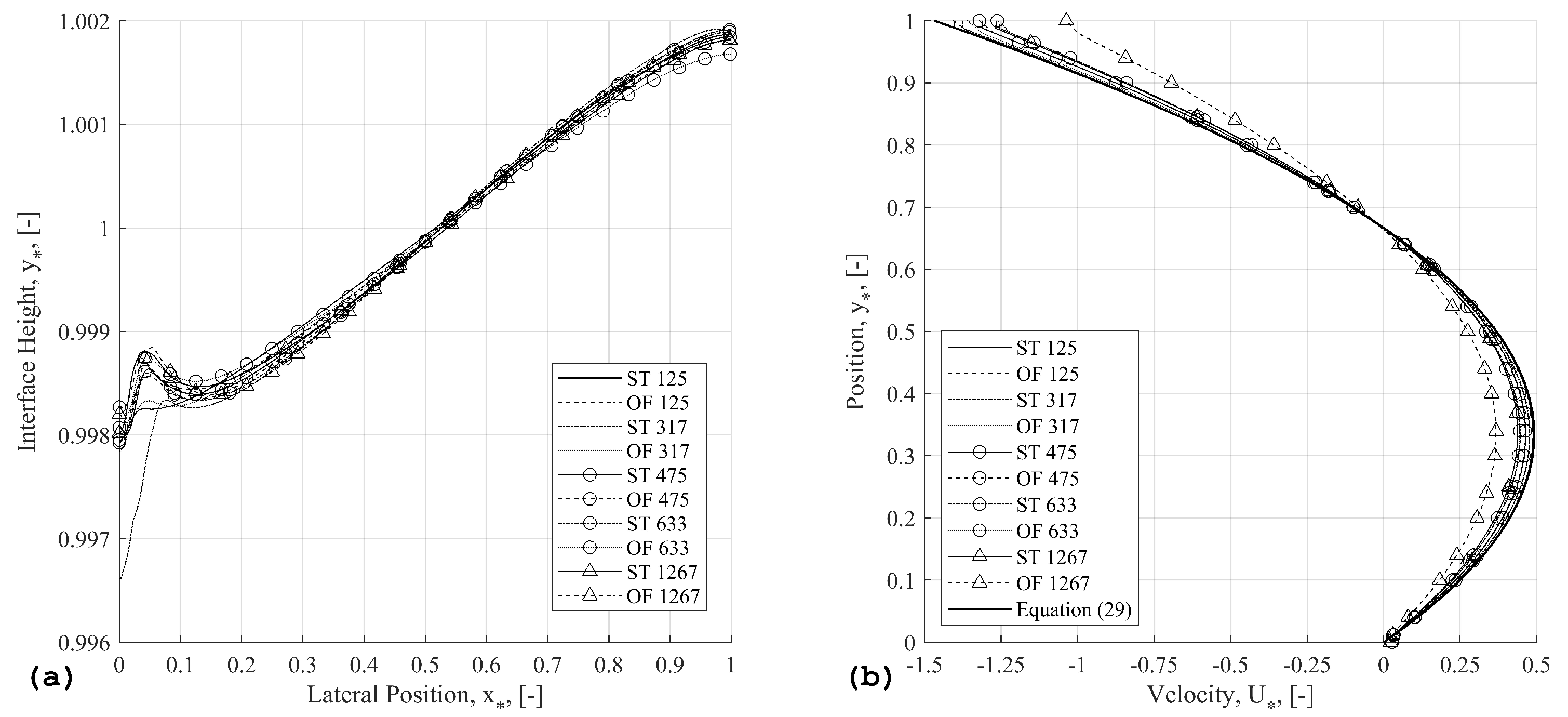
Figure 2.
Effect of Marangoni number on interface position in S3 (a) and velocity profile in S3 (b), predictions from STAR-CCM+ (ST) and openFOAM (OF). The number beside each label is the Marangoni number.

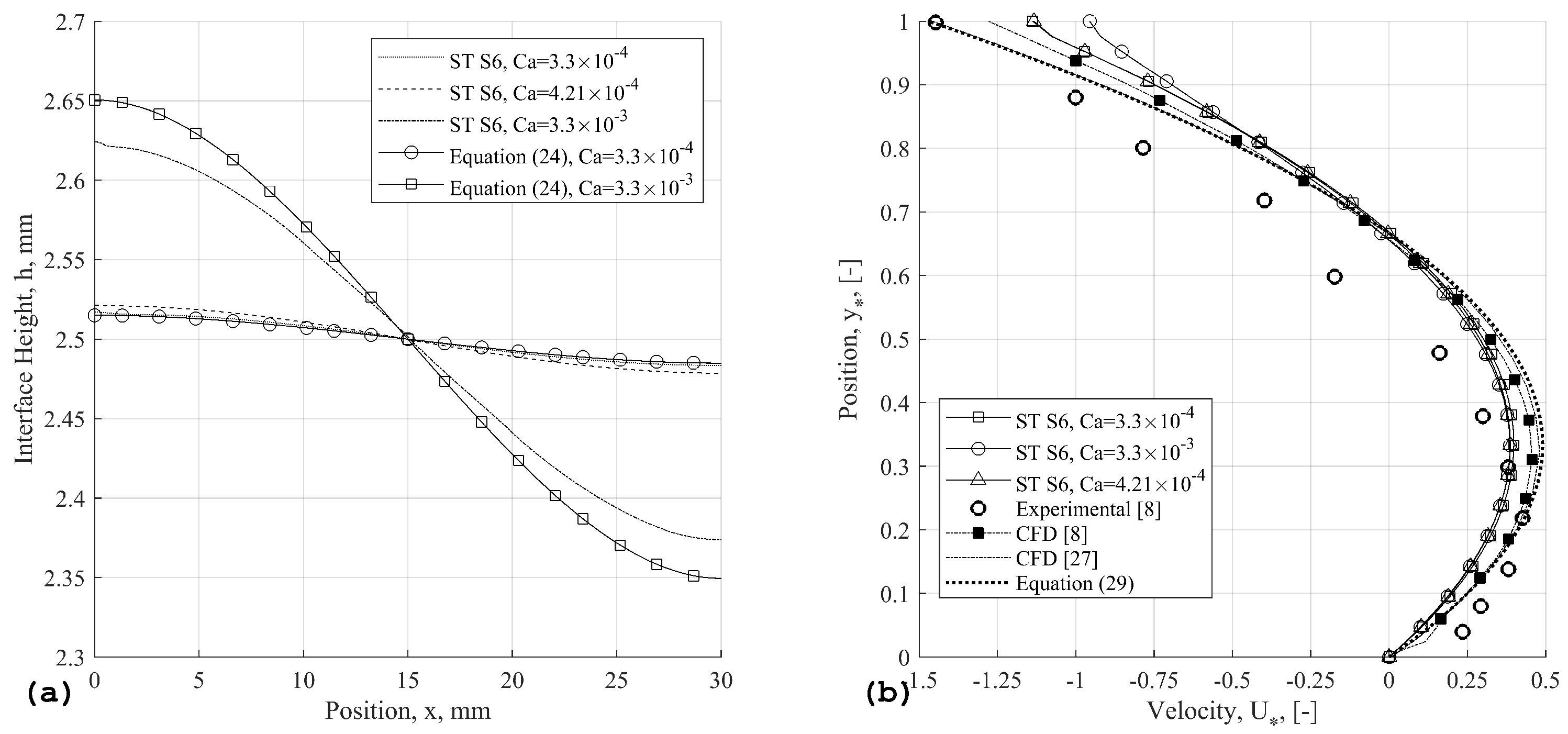
Figure 3.
Effect of Capillary Number on interface position (a), and velocity profile at (b) in S6, constant Marangoni number 633, predictions from STAR-CCM+ (ST).
This expression, (29), comes with all the limitations and assumptions of the original expressions from Sen and Davis [7], as such it can only predict the liquid velocity profile and not the vapor velocity, nor effects near the sidewalls. A more generalized velocity profile for any value of uses a cubic profile [18]. An expression similar to (29) can be also be obtained for positive based on their approach. However, the recovery of the magnitude would require some additional work as it is not independent of Ma. In the present work, only (29) based on the work from Sen and Davis [7] will be compared to the results.
To scale our CFD results and previous experiments a slightly different velocity scale must be used which will be defined as
while possibly controversial to use multiple velocity scales, (30) is a physical velocity scale that represents the magnitude of convection in the problem based on the balance of forces. Whereas (28) is more of a numerical scaling factor to apply to the analytical expression in (27).
4. CFD
In both STAR-CCM+ [32] and openFOAM [33], the PISO and SIMPLE methods are used for solving the governing equations. Initial conditions and boundary conditions are described in Section 2.3. Relaxation factors and solver settings were left as default in both models. Contact angles on all boundaries were set at 90 deg. Material properties were set according to Table 1 and Section 2.2. All cases were laminar and used a isotropic hexahedral grid for the domain. Previous work found grid independence on this flow problem with coarser grids [27]. While some results are presented as nondimensional (or scaled dimensionally when relevant for comparison), the CFD models solve the dimensional form of the governing equations, and a domain size of m was used, giving a grid sizing ∼1.66 mm.
Both openFOAM and STAR-CCM+ are studied and compared throughout this work to demonstrate that the chosen isothermal benchmark can be easily setup and compared across codes. The motivation is to encourage future developed codes or approaches for Marangoni flows to use the same benchmark with confidence.
4.1. STAR-CCM+ Setup
STAR-CCM+ provides an intuitive menu for selection of the desired physics that adapts the options available based on the previous selection. Models were chosen to replicate those in openFOAM. In the present work, the VOF model was selected which requires the ‘multiphase model’ and the segregated solver (SIMPLE family of solvers). The space model was two-dimensional, and the gravity model was also selected. For energy conservation, the ‘Segregated Multiphase Temperature’ model is used. Within phase interactions, the surface tension model was selected with Marangoni convection enabled.
4.2. openFOAM Implementation
The tangential surface tension force, (21), was implemented in openFOAM v2106 using the solver compressibleMultiphaseInterFoam as the starting point for development in the present work. This is an N-phase compressible solver that includes effects models of constant normal surface tension, and wall contact angle. This solver uses the openFOAM thermophysical properties library and many combinations of equations of state are possible.
Using the VOF method introduces an additional caveat for interface calculations. The interface normal vectors for both phases must be considered as all phases share a pressure field and only one continuity equation is solved. Equation (21) is still valid in its current form, however is slightly different and will contain the volume fraction gradients (the interface normals) of both phases. In Algorithm 1, line 2, the calculated interface normal vector field is demonstrated.
In addition to the VOF complications, the solver uses the finite volume method (FVM). Special care must be taken to ensure distinction from cell centered values (referred to in openFOAM parlance as volume fields) and face centered values (surface fields). Any scalar or vector quantities can be converted freely between the volume and surface data types. For example, a volume-scalar can be converted to a surface-scalar via interpolation from mesh centroids to the cell faces. A volume-vector can be projected from the mesh centroids onto the cell faces, giving a flux at the cell face and a surface-scalar.
After constructing the tangential surface tension force from (21) in line 4, the volume-vector is then converted to a surface-scalar by taking the inner product with the cell face normals. The algorithm then steps the relevant calculations from Section 2.5. For more details on the implementation, the full source code along with a few example cases are available on GitHub [38].
| Algorithm 1 Calculate Surface Tension Force |
|
5. Results
The steady state timescale for the numerical solution is estimated based on a fluid parcel moving at the characteristic velocity from (30) over the domain length L around five times. This gives a physical time of around 15–25 s. For most cases, a time-step of s was used without stability problems. Running the simulations with 4 CPUs required around 10 min wall time per case.
In total ten scenarios were considered, each with different combinations of physics, boundary conditions or equations of state. In Table 2, the cases investigated are summarized. With S1–S6, the liquid density was held constant, while in S1B–S4B the liquid density was varied according to (23). In S5 and S6, the vapor and liquid densities were constant, and in all other scenarios the ideal gas law was used for vapor. S1–S4 examine the effect of gravity and the top boundary condition. The open domain refers to a symmetry condition at the top-wall from Figure 1, while a closed domain refers to a no-slip top wall boundary condition. Either gravity was completely removed, or terrestrial gravity was applied, , in the y direction from Figure 1. S5 and S6 examine a completely incompressible fluid and the effects of the top boundary. The effects of buoyancy in the liquid phase was considered in S1B–S4B each of which align with S1–S4 respectively.
Table 2.
Summary of Scenarios Investigated.
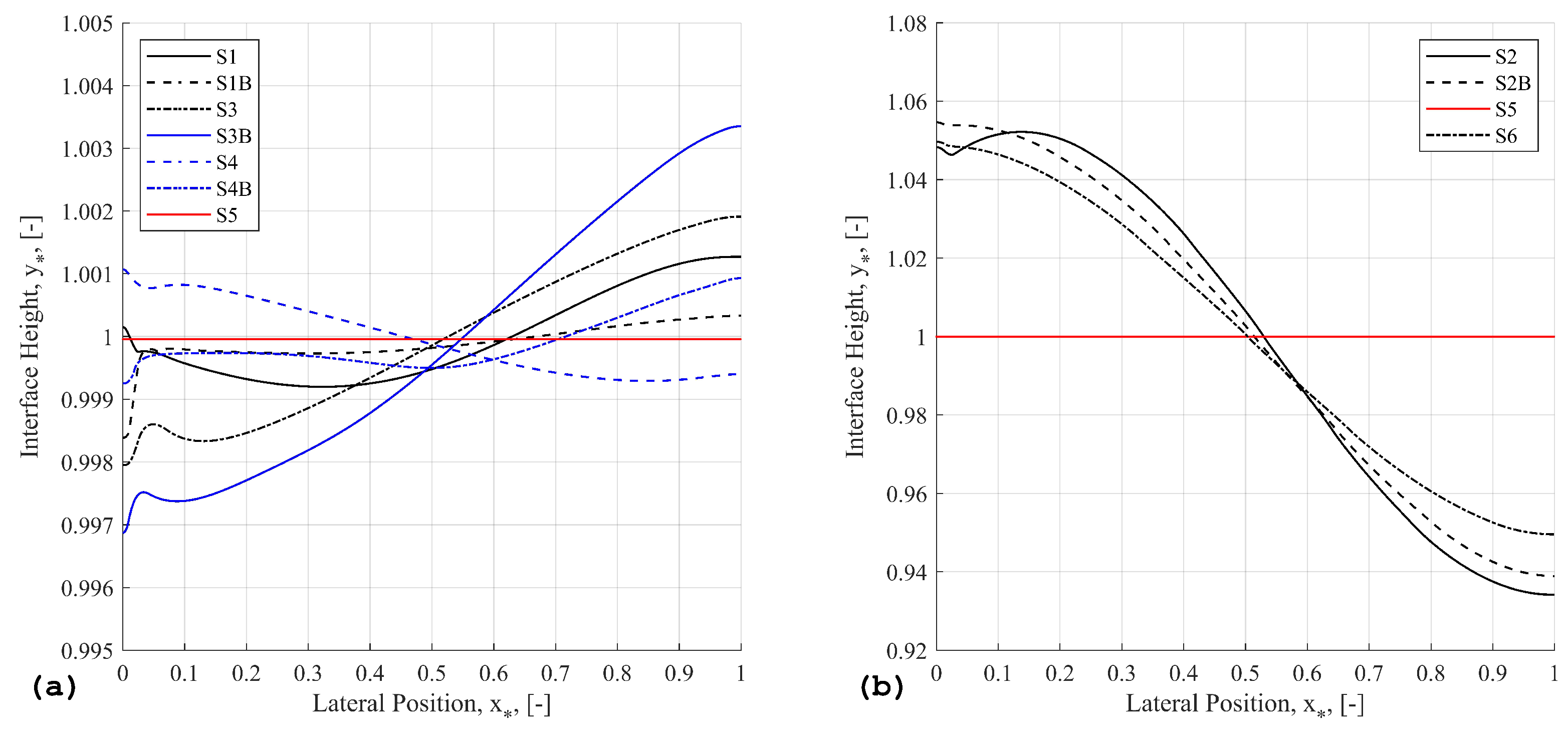
The interface is taken as the isosurface . The orientation was defined as the change in average interface height with respect to the positive x direction (if the free surface generally rises moving right, the orientation is considered positive). In nearly every simulation, interface smearing was found near the cold wall at , as shown in Figure 2 and Figure 4. While this is concerning, mass was still conserved to a high degree in every case (< kg lost). Second and third order schemes were tried but with small reductions in smearing for longer run times. The most likely explanation is the compressible formulation used in the VOF method, as incompressible scenarios have this issue to a lesser degree as seen from S5 and S6 in Figure 4. STAR-CCM+ does have several interface sharpening methods available (HRIC, multi-stepping, etc.), but these were not investigated.
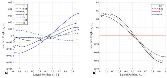
Figure 4.
Interface height in different scenarios, constant Ma number 633, predictions from STAR-CCM+. (a) cases with small deformations, (b) cases with large deformations, S5 included for visual reference only. Note the difference in scale on the y-axis.
If future work finds the interface smearing from VOF to be problematic, then other multiphase methods such as the isoAdvector or level-set approaches can be tested. However, as mass was conserved to a high degree, and the relevant physics were captured accurately compared to previous results, the VOF method with CSF implementation used presently is concluded to be more than sufficient to model the effects of Marangoni convection.
5.1. Effect of Marangoni Number
The interface height for S3 as described in Table 2 is shown over a range of Ma in Figure 2. There is not much change in the shape of the profile with the Marangoni number, and interface smearing is present near in every case, especially ST 317. However, in these nondimensional plots, the relative impact of the smearing is exaggerated greatly. The interface height at the left wall is ∼0.9965 mm versus the likely true value (based on symmetry) of ∼ mm, a difference of less than 4 m.
The right side of Figure 2 shows the corresponding liquid velocity profiles along the vertical direction taken at X = L/2, with the prediction from (29). In Figure 2, each velocity profile has a maximum at in agreement with the maxima of (29). A coefficient of is taken for (29) and matches the other results well. Only the openFOAM case with deviates from the pattern. This may be due to a difference in numerical implementation between STAR-CCM+ and openFOAM that only becomes apparent at higher Marangoni numbers. From these results, we can conclude that the openFOAM and STARCCM+ implementations of Marangoni convection are generally equivalent and yield similar results to the analytical expression.
5.2. Effect of Capillary Number
The expression for the interface height (24) from Sen and Davis [7] has various assumptions and is most applicable to S6 as described in Table 2. In Figure 3, the theoretical model from (24) indeed predicts the effect of capillary number well. Here the interface height has been dimensionalized with the nominal height of 2.5 mm. Two nominal cases were tested with . The third case with corresponds to the experiments from Villers and Platten [8] based on their experimental conditions and the material properties of acetone. This shows that a minor change in the capillary number (∼) does not change the height profile much, but an order of magnitude change does have an impact. ST S6 and (24) align very well for and differences are on the order of the line thickness. The numerical results are mostly within the confidence range from (24) of m. Disagreement with the theory can be attributed to the effects of the vapor phase which is not considered in the theoretical expression.
On the right side of Figure 3, the capillary number is shown to not have much effect on the velocity profile. The previous CFD shows some minor disagreement as the problem was modeled with a fixed flat interface and Marangoni forces were applied along the flat boundary [8,27]. Previous CFD results and (29) give a maximum while results from STAR-CCM+ in S6 give a maximum . Here, C is taken as 2 as well in (29) with good agreement. The experimental results from Villers and Platten [8] give a larger magnitude of for both the rightward and leftward velocities. This may be due to three-dimensional effects from their experiments. From this set of results, we can conclude that the implementation agrees well with the theory, experimental data, and the effect of capillary number is well captured.
5.3. Effect of Scenario
In Figure 4, the interface shape is plotted for all eight scenarios at a constant Marangoni number as described in Table 2. If the simulations were perfect, each line would be mirrored about and intersect due to the symmetry of the problem. This again shows the smearing limitations of the VOF method. In Table 3 and Table 4, the key results from each scenario are summarized.
Table 3.
Results of scenarios.
Table 4.
Results of scenarios, velocity comparison.
Looking at the zero-gravity cases, S1 and S2, significantly different results are obtained. With a no-slip wall top boundary condition as in S1, the interface orientation is positive and overall deformation is small. With a symmetry boundary as in S2, the orientation is negative and deformation is nearly 50 times larger as shown by the maximum height listed for S1 and S2 in Table 3. This happens because in S1, the vapor expansion near the heated right wall is additional source of fluid motion acting in combination with the thermal gradients at the interface (Marangoni effect). When the domain is open, as in S2, the domain is at constant pressure and the thermal gradients along the interface dominate over the vapor expansion, giving a reversal in the interface deformation. This implies that a negative orientation of the free surface is the natural state under Marangoni convection. This is confirmed by the results of S6, where only Marangoni forces are acting on the interface because both phases are constant density. S6 is the most representative of the setup studied by Sen and Davis [7] and the orientation and magnitude of the interface deformation matches their theoretical model, see Figure 3 and Figure 4.
If both phases are constant density, S5 and S6, then gravity plays no role at all. Results show that in S5, there is no interface deformation at all, as in Figure 4, and the peak velocity is higher than in S1 which used the ideal gas law. Forcing both phases to be incompressible completely suppresses interface deformation and increases the overall convection rates. With the domain open, S6, the deformation and velocities are similar to those from S2.
Interface reversal due to the top wall boundary condition has been noted before. In Zhou and Huang [22], the authors modeled two immiscible species and commented that “the interface deformation orientation of the analytical solution by Sen is opposite to the present simulation, which is due to the density and viscosity of the upper layer fluid [which] is ignored in Sen’s research”. However, the present results show this to be only partially true.
Comparing S1 and S5, we can conclude the vapor equation of state allows the interface to deform in closed domains. However, in open domains, S2 and S6, there is little effect due to the dominance of Marangoni forces over the heated vapor expansion. From the results of S1–S4, the reversal (a positive orientation) only occurs with a closed domain and with a compressible vapor phase. It is thus vapor expansion within a closed domain that drives the reversal. The vapor expansion near the hot wall creates additional convection leftward to the cold wall. Near the cold wall, there must be a mass imbalance that is equalized by the interface receding from the cold wall.
This highlights that the use of the correct top wall boundary condition is critical to modeling and predicting the magnitude of the interface deformation, as well as the resulting liquid velocity scale. In practical applications this would lead to very different heat transfer predictions. For example, heat pipes are a closed domain and the results from S1 or S3 would more appropriately describe the physics there, and results would give a small positive deformation. Whereas in an application like metal welding an open domain is more representative, S2 or S4 would be more appropriate, and a large negative deformation is possible.
5.3.1. The Liquid Equation of State
To remove an assumption of constant liquid density, liquid thermal expansion was accounted for using (23) in scenarios with names appended with ‘B’ as described in Table 2. Again due to the limitations of the VOF method, interface smearing limits the comparison of interface height in ‘B’ scenarios as the differences are small. The exception is scenarios S4 and S4B, where the interface orientation reversed from a negative orientation to a positive one with liquid expansion. This shows that in addition to the reversal found in the previous section, another mechanism exists by changing the liquid equation of state.
In all these cases, differences in peak velocities were discernible and each ‘B’ scenario had a lower maximum velocity as shown by Table 4. Interestingly, in S4 and S4B, the peak velocity dropped by nearly 16%, in addition to the interface flipping orientation solely by changing the liquid density to a linear function of temperature.
The conclusion here is that including more physics (removing an assumption) changes the results significantly. This shows that selection of simplifications is critical in modeling Marangoni convection. This may seem abstract, but in a heat transfer analysis a difference in the convective velocity scale of more than 15% due to the liquid equation of state is quite concerning. Additionally, the fact that this change occurs only in some scenarios shows that the combination of boundary conditions and chosen equations of state significantly impact the results of the model.
5.3.2. Impact on Velocity Profiles
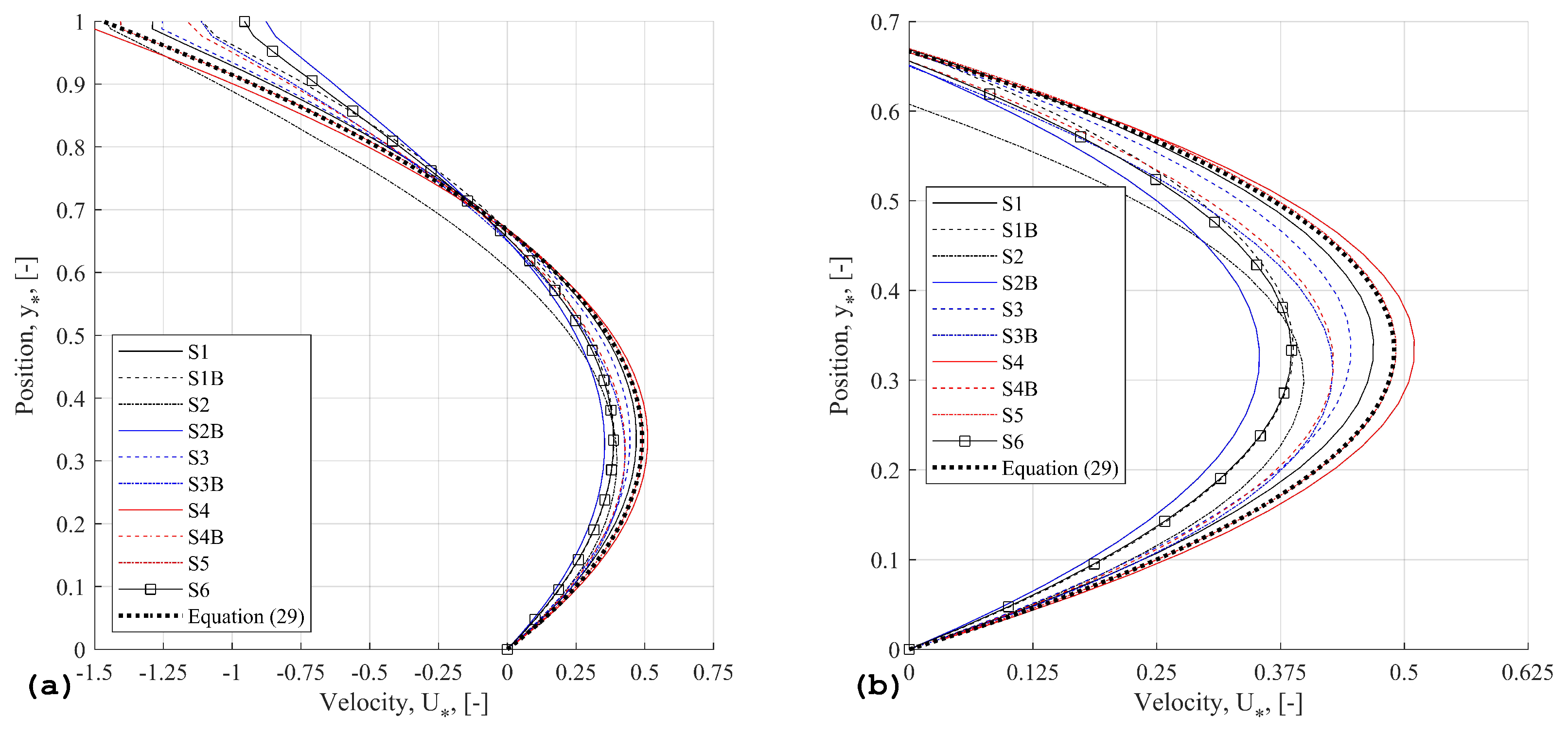
In Figure 5, the velocity profiles from each scenario are plotted together with a constant Marangoni number as described in Table 2. With the left view, each scenario follows the same parabolic trend with increasing height. In the right view, the difference between scenarios is more clear, but there is no obvious grouping. All scenarios have their peak velocity at the maxima of (29) as , except for S2, S3, and S3B, which are closer to . The maximum ranges from in S4 down to in S2B.
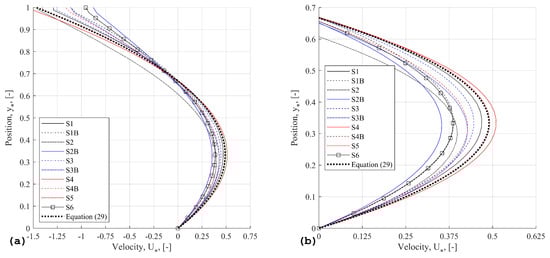
Figure 5.
Velocity profiles at in different scenarios, constant Marangoni number of 633, results from STAR-CCM+. Full profile (a) and zoomed (b).
Whether the domain was open had a large impact on the peak velocity, as shown by the “Open/Closed diff” column in Table 4. In scenario S6, the velocity was reduced by more than 20% compared to S5. Yet with S3 and S4, the velocity was actually increased in the open scenario. Liquid thermal expansion reduced the velocities in all cases, but S1B had showed the greatest impact, reducing by 17%. This is shown in the “ diff” column of Table 4. Consideration should also be given to the effect of buoyancy (in both phases) as the velocities change significantly. In Table 4, the ‘Gravity diff’ column shows the percentage change in the peak velocity under one-g relative to zero-g. For example, S1 and S2 are compared against S3 and S4 respectively as the only difference is gravity, and similarly for the “B” cases. Most velocities increased with increasing gravity, and S4 had the largest change increasing by 28% over S2. However, S3 had a slight decrease over S1 and its unclear why. Especially after considering results of S3B, which showed an increase over S1B.
6. Conclusions
Due to the many industrial uses for Marangoni flows, it is critical for a numerical model to capture the behavior correctly for accurate predictions. In single phase flows, benchmarks like the lid driven cavity have become standard and recognized as fundamental tests for a newly developed CFD code. For multiphase free surface flows with variable surface tension, the presently studied pool with isothermal sidewalls was proposed as it is the simplest domain where Marangoni effects can dominate. It was also chosen due to its strange sensitivity to the initial setup which was discussed at length from a chosen number of ‘scenarios’.
In short, strong caution should be taken in simplification of Marangoni flows. It was found that the fluid interface can reverse deformation by a change in the top boundary condition, the liquid equation of state, and gravity level. The interface reverses meaning that rather than climbing the cold wall, the interface climbs the heated wall. For the top boundary condition, this reversal is due to vapor expansion within the closed volume, which adds a convection mechanism and drives the interface down from the cold wall. Not only does the interface reverse, but the peak height ranges by more than an order of magnitude at the same Marangoni number depending on the top wall boundary (see S1 vs. S2 results). To complicate matters further, the velocity scales can also change significantly. By changing to an open domain, the peak velocity can increase by up to 14% (see S4 vs. S2), or decrease by 21% (see S6 vs. S5). When including gravity, the peak velocity can increase by up to 27% (see S4 vs. S2 results), but it can also decrease when also changing the top boundary condition (see S3 vs. S1 results). Finally, by allowing thermal expansion of the liquid phase, the peak velocity is reduced in the range of 4% to 17% depending on the gravity and top wall (see S1B–S4B results).
These differences could lead to significant errors in analyzing a practical application. Take for example the simplest setup, an open domain, neglecting gravity, and taking constant density for both phases. The results would be inline with those of S6. However, if you remove those assumptions, the setup is then similar to S4B. The interface deformation becomes 50 times smaller and in the opposite orientation, and the velocity scale increases by more than 10%. Needless to say, this would introduce problems in a practical design analysis of heat transfer. Therefore, it is important to not only show that a new CFD code can resolve Marangoni convection, but also to demonstrate that the code can resolve the scenario most relevant to the application at hand. For general purpose benchmarking, scenario S6 and S3B are recommended. S6 has the largest interface deformation and corresponds with the previous analytical solutions. It also has the simplest setup with constant material properties, an open top boundary condition and no gravity. S3B is also recommended as it is the most complex setup and has interface deformation in the opposite direction from S6. S3B has a closed top boundary, gravity of 1 g, and variable liquid density. A successful benchmark of these two scenarios, S3B and S6, should give future researchers confidence that their implementation is sufficient to resolve Marangoni convection.
Future Work and Limitations
The interface reversals and changes in velocity scales described in Section 5.3 were studied at a constant Marangoni number of 633. Considering that the changes in results were sporadic with a single parameter change, adjustments in the Marangoni number will likely also change the findings. Future work should investigate scenarios S1–S6 and S1B–S4B over a range of Marangoni number, domain aspect ratio, and intermediate gravity levels. Further work could study the effect of reverse Marangoni convection in fluids with . Additionally, these setups should be tested with multiple species and concentration effects, isolation of the Prandtl number, and Prandtl number ratio between phases. Additional experimental datasets that isolate other physics phenomena would also be of great value for improving the scope of this benchmark. For example, including a solid melt phase or different thermal boundary conditions than those studied here could help generalize the benchmark for other applications.
Author Contributions
Conceptualization: B.E.C.; Data curation: B.E.C.; Formal analysis: B.E.C.; Funding acquisition: B.E.C. and C.S.B.; Investigation: B.E.C.; Methodology: B.E.C.; Project administration: C.S.B.; Resources: C.S.B.; Software: C.S.B.; Supervision: C.S.B.; Validation: B.E.C.; Visualization: B.E.C.; Writing—original draft: B.E.C.; Writing—review and editing: B.E.C. and C.S.B. All authors have read and agreed to the published version of the manuscript.
Funding
This research was funded by the US Department of Energy, as part of a University Nuclear Leadership Program Graduate Fellowship under grant number NE0009076.
Institutional Review Board Statement
Not applicable.
Informed Consent Statement
Not applicable.
Data Availability Statement
The modifications to openFOAM are provided on github [38]. Example cases from STAR-CCM+ are also provided. Data for plots in the paper are available upon request from the authors.
Acknowledgments
This material is based upon work supported under a Department of Energy, Office of Nuclear Energy, Integrated University Program Graduate Fellowship. Any opinions, findings, conclusions, or recommendations expressed in this publication are those of the authors and do not necessarily reflect the views of the Department of Energy Office of Nuclear Energy.
Conflicts of Interest
The authors report no conflict of interest.
References
- Li, C.; Zhao, D.; Wen, J.; Lu, X. Numerical investigation of wafer drying induced by the thermal Marangoni effect. Int. J. Heat Mass Transf. 2019, 132, 689–698. [Google Scholar] [CrossRef]
- Mills, K.C.; Keene, B.J.; Brooks, R.F.; Shirali, A. Marangoni effects in welding. Philos. Trans. R. Soc. London. Ser. Math. Phys. Eng. Sci. 1998, 356, 911–925. [Google Scholar] [CrossRef]
- Schwabe, D.; Scharmann, A. Some evidence for the existence and magnitude of a critical marangoni number for the onset of oscillatory flow in crystal growth melts. J. Cryst. Growth 1979, 46, 125–131. [Google Scholar] [CrossRef]
- Mukherjee, T.; Manvatkar, V.; De, A.; DebRoy, T. Mitigation of thermal distortion during additive manufacturing. Scr. Mater. 2017, 127, 79–83. [Google Scholar] [CrossRef]
- Srimuang, W.; Amatachaya, P. A review of the applications of heat pipe heat exchangers for heat recovery. Renew. Sustain. Energy Rev. 2012, 16, 4303–4315. [Google Scholar] [CrossRef]
- Nguyen, T.T.; Yu, J.; Wayner, P.C.; Plawsky, J.L.; Kundan, A.; Chao, D.F.; Sicker, R.J. Rip currents: A spontaneous heat transfer enhancement mechanism in a wickless heat pipe. Int. J. Heat Mass Transf. 2020, 149, 119–170. [Google Scholar] [CrossRef]
- Sen, A.; Davis, S. Steady thermocapillary flows in two-dimensional slots. J. Fluid Mech. 1982, 121, 163–186. [Google Scholar] [CrossRef]
- Villers, D.; Platten, J. Coupled buoyancy and Marangoni convection in acetone: Experiments and comparison with numerical simulations. J. Fluid Mech. 1992, 234, 487–510. [Google Scholar] [CrossRef]
- Engberg, R.F.; Wegener, M.; Kenig, E.Y. The influence of Marangoni convection on fluid dynamics of oscillating single rising droplets. Chem. Eng. Sci. 2014, 117, 114–124. [Google Scholar] [CrossRef]
- Qin, T.; Tuković, Z.; Grigoriev, R.O. Buoyancy-thermocapillary convection of volatile fluids under their vapors. Int. J. Heat Mass Transf. 2015, 80, 38–49. [Google Scholar] [CrossRef]
- Cao, L. Mesoscopic-scale simulation of pore evolution during laser powder bed fusion process. Comput. Mater. Sci. 2020, 179, 109686. [Google Scholar] [CrossRef]
- Samkhaniani, N.; Stroh, A.; Holzinger, M.; Marschall, H.; Frohnapfel, B.; Wörner, M. Bouncing drop impingement on heated hydrophobic surfaces. Int. J. Heat Mass Transf. 2021, 180, 121777. [Google Scholar] [CrossRef]
- Sabanskis, A.; Virbulis, J. Simulation of the influence of gas flow on melt convection and phase boundaries in FZ silicon single crystal growth. J. Cryst. Growth 2015, 417, 51–57. [Google Scholar] [CrossRef]
- Hadid, H.B.; Roux, B. Thermocapillary convection in long horizontal layers of low-Prandtl-number melts subject to a horizontal temperature gradient. J. Fluid Mech. 1990, 221, 77–103. [Google Scholar] [CrossRef]
- Roux, B. (Ed.) Numerical Simulation of Oscillatory Convection on Low-Pr Fluids; Vieweg+Teubner Verlag: Berlin, Germany, 1990. [Google Scholar] [CrossRef]
- Hadid, H.B.; Roux, B. Buoyancy- and thermocapillary-driven flows in differentially heated cavities for low-Prandtl-number fluids. J. Fluid Mech. 1992, 235, 1. [Google Scholar] [CrossRef]
- Bergman, T.L.; Keller, J.R. Combined Bouyancy, surface tension flow in liquid metals. Numer. Heat Transf. 1988, 13, 49–63. [Google Scholar] [CrossRef]
- Villers, D.; Platten, J. Separation of Marangoni convection from gravitational convection in earth experiments. Physicochem. Hydrodyn. 1987, 8, 173–183. [Google Scholar]
- Sasmal, G.P.; Hochstein, J.I. Marangoni Convection with a Curved and Deforming Free Surface in a Cavity. J. Fluids Eng. 1994, 116, 577–582. [Google Scholar] [CrossRef]
- Kothe, D.; Francois, M.; Sicilian, J. Modeling of thermocapillary forces within a volume tracking algorithm. In Proceedings of the Modeling of Casting, Welding and Advanced Solidification Processes—XI, Opio, France, 28 May–2 June 2006; Volume 2. [Google Scholar]
- Bauer, H.; Eidel, W. Thermo-capillary convection in various infinite rectangular container configurations. Heat Mass Transf. 2003, 40, 123–132. [Google Scholar] [CrossRef]
- Zhou, X.; Huang, H. Numerical Simulation of Steady Thermocapillary Convection in a Two-Layer System Using Level Set Method. Microgravity Sci. Technol. 2010, 22, 223–232. [Google Scholar] [CrossRef]
- Zhou, X.; Huai, X. Numerical Investigation of Thermocapillary Convection in a Liquid Layer with Free Surface. Microgravity Sci. Technol. 2014, 25, 335–341. [Google Scholar] [CrossRef]
- Zhou, X.; Liu, Z.; Huai, X. Evolution of free surface in the formation of thermo-solutocapillary convection within an open cavity. Microgravity Sci. Technol. 2016, 28, 421–430. [Google Scholar] [CrossRef]
- Zhou, X.; Huai, X. Influence of thermal and solutal Marangoni effects on free surface deformation in an open rectangular cavity. J. Therm. Sci. 2016, 26, 255–262. [Google Scholar] [CrossRef]
- Saldi, Z.S. Marangoni Driven Free Surface Flows in Liquid Weld Pools. Ph.D. Thesis, Delft University of Technology, Delft, The Netherlands, 2012. [Google Scholar] [CrossRef]
- Chen, E.; Xu, F. Transient Marangoni convection induced by an isothermal sidewall of a rectangular liquid pool. J. Fluid Mech. 2021, 928, A6. [Google Scholar] [CrossRef]
- Tan, L.H.; Leonardi, E.; Barber, T.J.; Leong, S.S. Experimental and numerical study of Marangoni convection in shallow liquid layers. Int. J. Comput. Fluid Dyn. 2005, 19, 457–473. [Google Scholar] [CrossRef]
- Kamotani, Y.; Ostrach, S.; Pline, A. Analysis of velocity data taken in Surface Tension Driven Convection Experiment in microgravity. Phys. Fluids 1994, 6, 3601–3609. [Google Scholar] [CrossRef]
- Montanero, J.M.; Ferrera, C.; Shevtsova, V.M. Experimental study of the free surface deformation due to thermal convection in liquid bridges. Exp. Fluids 2008, 45, 1087–1101. [Google Scholar] [CrossRef]
- Schwabe, D.; Scharmann, A. Marangoni convection in open boat and crucible. J. Cryst. Growth 1981, 52, 435–449. [Google Scholar] [CrossRef]
- Simcenter STAR-CCM+, version 2206.001; Siemens Digital Industries Software: Plano, TX, USA.
- openFOAM, verson 2106; OpenCFD: Reading, UK.
- Brackbill, J.; Kothe, D.; Zemach, C. A continuum method for modeling surface tension. J. Comput. Phys. 1992, 100, 335–354. [Google Scholar] [CrossRef]
- Simcenter STAR-CCM+ User Guide, version 2206.001; Siemens Digital Industries Software: Plano, TX, USA.
- Scheufler, H.; Roenby, J. TwoPhaseFlow: An OpenFOAM based framework for development of two phase flow solvers. arXiv 2021, arXiv:2103.00870. [Google Scholar]
- Scriven, L. Dynamics of a fluid interface Equation of motion for Newtonian surface fluids. Chem. Eng. Sci. 1960, 12, 98–108. [Google Scholar] [CrossRef]
- Ciccotosto, B. GitHub Repository. cmiFoam with Marangoni. 2022. Available online: https://github.com/brucethemuce/compressibleMultiphaseInterFoam_Marangoni (accessed on 13 July 2022).
Disclaimer/Publisher’s Note: The statements, opinions and data contained in all publications are solely those of the individual author(s) and contributor(s) and not of MDPI and/or the editor(s). MDPI and/or the editor(s) disclaim responsibility for any injury to people or property resulting from any ideas, methods, instructions or products referred to in the content. |
© 2023 by the authors. Licensee MDPI, Basel, Switzerland. This article is an open access article distributed under the terms and conditions of the Creative Commons Attribution (CC BY) license (https://creativecommons.org/licenses/by/4.0/).