Abstract
As a type of airtight equipment, vertical gas tanks are prone to accumulations of toxic and harmful gases due to their poor ventilation and narrow space. This poses many safety hazards. Therefore, we conducted a FLUENT simulation for vertical gas tanks with different diameters. The results indicated that the larger the diameter, the longer the required ventilation time. It was necessary to monitor the gas concentration after ventilation for at least 6 h when the tank diameter was 2.6 m, after ventilation for at least 24 h when the tank diameter was 5.2 m, and after ventilation for at least 80 h when the tank diameter was 7.8 m. To ensure comprehensive monitoring, at least one monitoring point was required to be placed at the upper and lower ends of the vertical gas tank, respectively. Monitoring was initiated after these requirements were reached. A theoretical numerical analysis and an experimental verification analysis were conducted on the simulation results. The variation trend of the simulation value, the theoretical value, and the experimental test value were the same. The measured value of the ventilation duration was greater than the theoretical value of the ventilation duration and the simulation value of the ventilation duration. Therefore, the simulation results and theoretical analysis could be used for a risk analysis of gas tanks. The determination of ventilation characteristics via a simulation of vertical gas tanks has a practical significance when guiding on-site operations.
1. Introduction
Confined spaces present entry and exit difficulties for workers; these must be accessible enough to permit short-term work. A confined space has the characteristics of poor ventilation, no exchange of gas with the outside world, a narrow internal activity range, high humidity, and high temperatures. These can easily lead to the formation and accumulation of toxic and harmful substances, presenting many safety hazards, damaging the health of workers, and even threatening life [1]. As a type of confined space, a gas tank is more prone to accidents due to the existence of toxic and harmful gases that are difficult to discharge during maintenance work as well as other processes inside the tank. To enable construction personnel to work in a safe environment [2], it is necessary to ensure the proper ventilation of gas tanks during various operations. If there is no ventilation or if improper ventilation methods are used, personnel may be poisoned, or fire and explosion accidents may occur [3]. To ensure correct ventilation conditions, it is important to master the gas transport characteristics of different types of gas tanks to guarantee the safety of operations. This includes the maintenance of the tank, for example.
Domestic and international scholars have undertaken research on gas migration laws in confined spaces. Li Qiu et al. [4] used a numerical simulation to study the leakage law of methane gas in a confined space. They concluded that a confined space was the area where methane easily accumulated, and an unconfined space was the area where methane did not easily accumulate. Tan Cong et al. [5] used a numerical simulation to study the distribution laws of different gases in confined spaces during the ventilation process. They concluded that a necessary volume of oxygen should be used during the actual work process. A score was used as a key parameter to measure the ventilation effect. Yang Xinjian et al. [6] used computational fluid software to conduct a three-dimensional numerical simulation of a forced ventilation gas flow when a single-manhole pressure vessel was shut down. In other cases, it was difficult to replace the internal gas. Yang Chunli et al. [7] used a numerical simulation to study the external wind speed, external wind direction, and composition of toxic and harmful gases in a confined space and influence of the type of confined space on the natural ventilation effect. Li Guoqing [8] used simulation software to numerically simulate the diffusion of harmful gases caused by ventilation during confined-space operations. Although ventilation helps to reduce the concentration of harmful gases, its effectiveness may be limited. Operators should take effective measures to prevent poisoning and fire explosions when working in a confined space. Chen Yang et al. [9] studied gas flows in confined spaces in the construction industry under different ventilation conditions. They concluded that the ventilation methods leading to the highest level of comfort for the human body were the upper-inward and lower-return methods. Yu Li [10] used a numerical simulation method to study the diffusion laws of urban natural gas pipelines. The influence of ventilation conditions on the concentration field in confined spaces was simulated. It was concluded that the higher the position of the vent and the greater the wind speed, the more favorable the diffusion of natural gas. Wang Zhihua [11] used a numerical simulation method to simulate a hydrogen tank in a ventilated room and studied the position of the vent and the effect of obstacles. There was an influence on the hydrogen concentration distribution and diffusion velocity field in the room. Li Xiangfu [12] used a numerical simulation method to study the diffusion laws of the leakage process of an LPG horizontal storage tank and summarized preventive measures in accordance with the laws. Quan et al. [13] studied ventilation methods for a cylindrical confined space. It is difficult to remove pollutants from this type of workspace using traditional ventilation methods. Therefore, a vortex ventilation model was proposed to ensure the safety of workers. The removal effect on lower pollutants was twice that of ordinary ventilation. Pouzou et al. [14] studied the ventilation effects of confined spaces in shipbuilding enterprises and observed the frequency of welding workers using ventilation, detecting their exposure to particulate matter. Zhao et al. [15] studied the migration of natural gas in tight reservoirs and Wei et al. [16] studied gas migration laws under underground mining conditions. Lu et al. [17] studied gas migration laws in goafs. To study the influence of obstacles, leakage speed, leakage direction, and wind speed on the leakage and diffusion laws of mixed gas, Schmidt [18] selected a hydrogen–oxygen mixed gas as the research object and used FLUENT to simulate the leakage and diffusion of the mixed gas. It was observed that the four indicators had a serious impact on the leakage and diffusion of the mixed gas. Spyros Sklavounos [19] used LNG and oxygen as research objects and simulated them using numerical software. In their diffusion situation, the quantitative relationship between the leakage time and the maximum gas concentration was analyzed and summarized; the research results were significant. Tauseef S M [20] studied the diffusion behavior of heavy gas in a diffusion environment with obstacles and analyzed the fluctuations in gas concentrations caused by gravity during the diffusion process. The results indicated that the realizable k-s model was more efficient than the standard k-ε model simulation, in terms of accuracy. To solve the problem that risks cannot be updated at any time in the process of a traditional dynamic risk assessment, researchers conducted a multi-angle analysis and proposed different solutions to obtain a dynamic assessment [21]. Meel et al. [22] developed a dynamic assessment method using event data to estimate the dynamic probability of an accident sequence to obtain a dynamic risk assessment of a system. Nicola et al. [23] proposed a dynamic risk management method that combined a risk concept and an early warning system that updated risks to prevent major accidents to enhance the identification of hazardous factors and generate real-time risk assessments. They verified the effectiveness of this method with specific dust explosion accidents. Kalantarnia et al. [24] used a dynamic risk assessment method to model the Texas City refinery accident. Rathnayaka et al. [25] applied Bayes theory to the system hazard identification, prediction, and prevention (SHIPP) methodology of LNG facilities.
Despite the existing research on gas migration in confined spaces aboveground and confined spaces underground, simulation research on gas migration in gas tanks with closed equipment causing poisoning, suffocation, and explosion accidents is limited. In this study, we first used the GAMBIT modeling method to model the tank body because of the gas concentration distribution problem in air tanks with closed equipment under ventilation states. Second, the FLUENT numerical simulation method was used to compare and study the gas concentration changes of different types of gas tanks with different diameters under ventilation conditions. Finally, theoretical prediction and experimental verification methods were used to analyze the operational risks of the gas tanks.
2. Simulation of Basic Assumptions and Establishment of Governing Equations
2.1. Basic Assumption
The gas migration process in a tank is affected by many environmental and internal factors. To simplify the workload of numerical simulations without affecting the simulation effect, our simulation assumed the following:
- (1)
- The internal structure of a gas tank in an actual working environment is complex. Therefore, it was necessary to simplify the geometric model used for the FLUENT simulation according to the data measured by different gas tanks. In other structures in gas tanks close to a wall, the influence of gas and wind flows in the tank was ignored to facilitate the calculation.
- (2)
- Storage tanks can be divided into three types, according to their external shape characteristics: vertical cylindrical storage tanks, with the circumferential surface of the tank body perpendicular to the ground; horizontal cylindrical storage tanks, with the central axis parallel to the ground; and tanks with a noncylindrical surface. Vertical cylindrical storage tanks are the most common in engineering [26]. Therefore, vertical tanks with different diameters were selected as the simulation objects. The specific dimensions and ventilation conditions are shown in Table 1. The air composition of natural ventilation is mainly oxygen and nitrogen. Therefore, the components of the external airflow were composed of oxygen and nitrogen. The oxygen concentration used was 21% and the nitrogen concentration was 79%. The content of other gases is very small; thus, they were ignored. The gas flow in a tank may be regarded as an incompressible fluid, and there is no chemical reaction of the gas in the tank; that is, the flow field space is regarded as an unsteady single-phase problem without a chemical reaction.
 Table 1. Different types of gas tanks and simulation conditions.
2.2. Governing Equation Establishment
In computational fluid dynamics, the governing equations used to describe multi-component three-dimensional unsteady turbulent flows have been established mainly according to the four laws of conservation of mass, conservation of momentum, conservation of energy, and conservation of component transport. Therefore, in this numerical simulation, the basic conservation law was followed in the numerical simulation settlement process [29,30,31,32].
- (1)
- Mass Conservation Equation
In describing fluid flow, the law that should be followed first is the law of mass conservation. The law of mass conservation is the basic law that mass transfer should obey. In the process of fluid flow, no matter what flows from the fluid, the total mass of the flowing fluid should be constant. The simulated fluid was deemed to be of a steady flow and an incompressible fluid; thus, the density of the fluid was a constant. Therefore, the law of conservation of mass was expressed as follows [33]:
where ρ is the fluid density; t is time; and u, v, and w are the projections of the velocity vector in x, y, and z directions, respectively.
- (2)
- Momentum conservation equation
The meaning of the law of conservation of momentum is that the action of the external force on the unit fluid micro-element will cause the fluid micro-element to generate momentum. The momentum of the fluid micro-element is equal to the rate of the change in the momentum of the fluid with time. This explanation is often referred to as Newton’s second law. In the equations in which this is expressed, it is also often referred to as the N-S equation [34]:
where ρ is the density; u, v, and w are the projections of the velocity vector in x, y, and z directions, respectively; μ is the dynamic viscosity coefficient of the fluid; and p is the unit of the fluid micro-element. The pressure of the shared body and the meanings of Su, Sv, and Sw are the generalized source terms of the momentum conservation equation.
- (3)
- Component mass conservation equation
Another control equation that was used in this numerical simulation experiment was the component transport equation, which mainly controls the change and hold of various gas concentrations during the transport of gas components in a porous medium. The component mass conservation equation can be expressed as follows [35]:
where cs is the volume concentration of the component S, ρcs is the mass concentration of the component volume, Ds is the component diffusion coefficient, and Ss is the component generation rate in the micro-element.
- (4)
- Energy conservation equation
The meaning expressed by this law is that the increased rate of energy in the micro-unit is equal to the net heat entering the micro-unit plus the work performed by the physical force and the surface force on the micro-unit. Its expression is as follows [36]:
where T is the ambient temperature, k′ is the heat transfer coefficient of the fluid, cp is the specific heat capacity of the fluid, and Sr is the heat source in the fluid and the heat generated by the viscous action during the fluid flow. The other symbols have the same meanings as above.
3. Mesh Model and Boundary Conditions
The grid size of a numerical simulation has a significant influence on the accuracy of the simulation and the computational efficiency [37]. Generally, the denser the grid spacing, the more accurate the calculation results. Therefore, it is necessary to determine the appropriate mesh size for specific problems during simulation calculations and to reduce the number of meshes as much as possible whilst ensuring the accuracy of the numerical simulation, thereby improving the calculation efficiency.
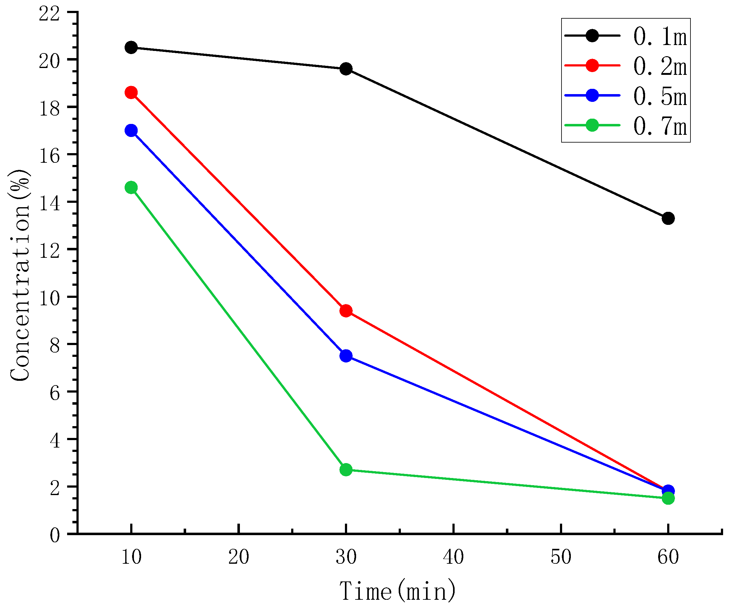
Due to the direct impact of the quality of the grid on the simulation results, it was necessary to conduct a comparative analysis of the density of the grids to be divided. The model area adopted a TGrid (tetrahedral grid) with four different sizes (0.1 m, 0.2 m, 0.5 m, and 0.7 m) selected for the interval size. The 0.1 m grid had a total of 1,213,789 grid cells, with a minimum grid area of 2.379 × 10⁻⁸ square meters. The 0.2 m grid had a total of 35,750 grid cells, with a minimum grid area of 1.89 × 10⁻⁶ square meters. The 0.5 m grid had a total of 11,076 grid cells, with a minimum grid area of 5.148 × 10⁻⁶ square meters. The 0.7 m grid had a total of 4348 grid cells, with a minimum grid area of 9.588 × 10⁻⁵ square meters. Through verification, we concluded from the entire process that the denser the grid, the slower it propagated. The 0.1 m grid required the longest time to ventilate until the carbon dioxide content was below 2%, followed by the 0.2 m grid. The shortest time required was for the 0.7 m grid, but the difference was not significant. On this basis, this simulation used the changes in carbon dioxide concentrations at different times at a central point at the height of the respiratory belt to further verify the grid independence (Figure 1).
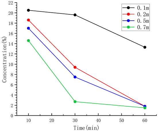
Figure 1.
Grid independence verification results.
When the grid size was reduced from 0.5 m to 0.2 m, the changes in carbon dioxide concentrations and the ventilation time required were similar. Based on the cloud image analysis results, we concluded that a grid size of 0.2 m reached grid quality independence. Taking into account the calculation time and accuracy, a grid quality of 0.2 m was selected for the subsequent numerical simulation.
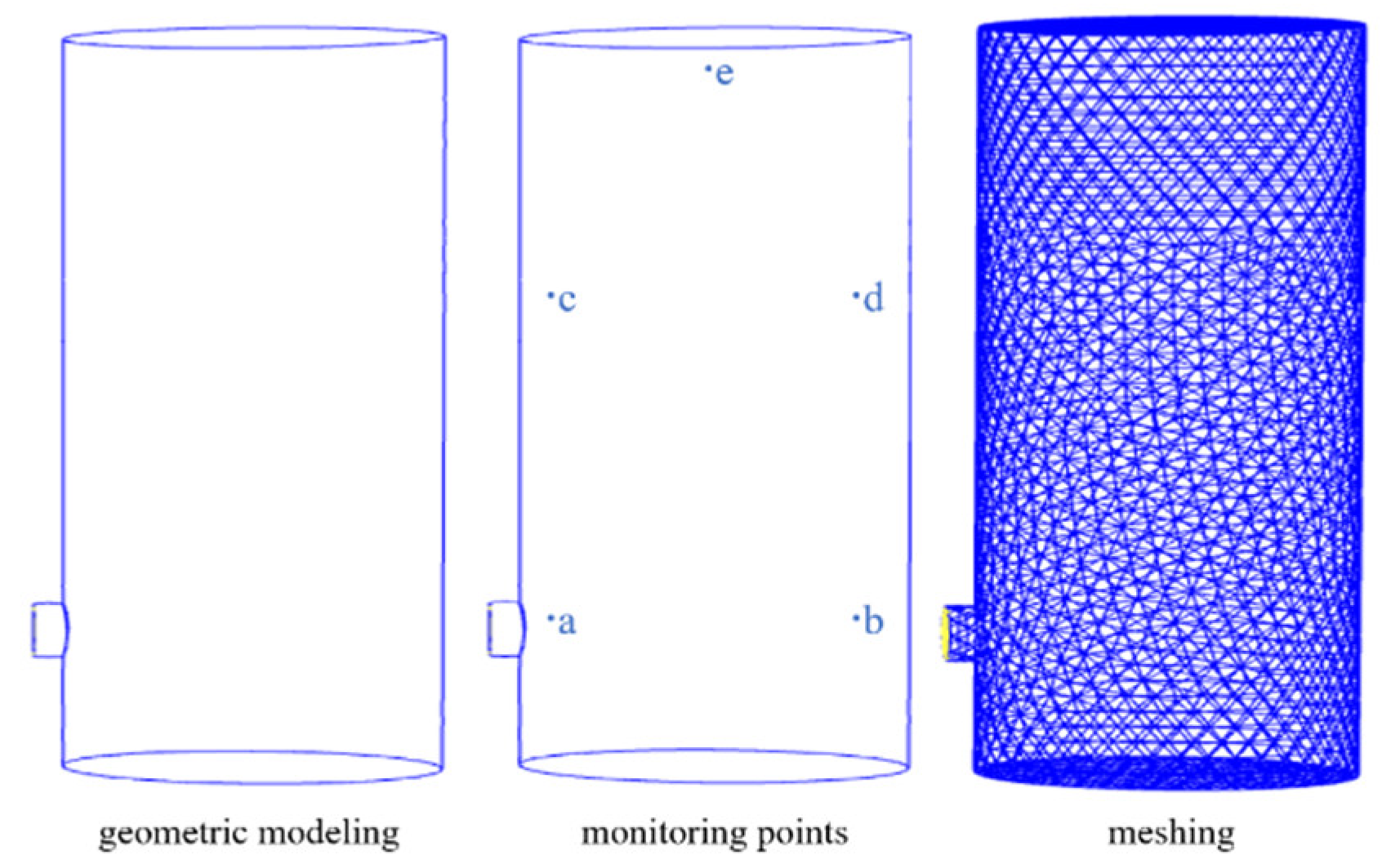
According to the design dimensions of gas tanks and their basic situation on-site, the main body of the gas tank we used was cylindrical with a diameter of 2.6 m and a height of 8 m. There was an inlet and outlet on the left side of the gas tank, which was a manhole for the easy entry and exit of workers. The diameter was 0.6 m and a 1:1 size simulation was used. Monitoring points were set at different positions inside the tank. Based on the above parameters, a three-dimensional model of a horizontal gas tank was established using GAMBIT [37] according to the simplified graphic size and shape. The calculation area used a TGrid (tetrahedral grid) and the interval size chosen was 0.2 m. The geometric model diagram, monitoring point bitmap, and divided grid schematic diagram are shown in Figure 2. By enlarging the model diagram and grid partition diagram in equal proportions two or three times, vertical gas tank models with tank diameters of 5.2 m and 7.8 m were also obtained, as well as a grid diagram.

Figure 2.
Air tank model and grid division.
The calculation method and mathematical model of FLUENT determined the parameters and boundary conditions of the numerical simulation, as shown in Table 2.
Table 2.
Computational model settings.
4. Simulation Results and Analysis
The results of the natural ventilation simulation were the vertical profile CO2 concentration distribution cloud figure and the CO2 concentration change line figure at the height of the breathing zone (z = 1.5 m) with horizontal incoming wind at different times. The longitudinal section was the center position of the tank along the incoming wind direction. The corresponding CO2 concentration change line graph formed a straight line along the height of the breathing zone parallel to the ground and 1.5 m above the ground. The numbers in the figure indicate the molar concentration of gas in the tank.
4.1. Simulation Results of Gas Migration in a Vertical, Single-Manhole, 2.6 m-Diameter Gas Tank
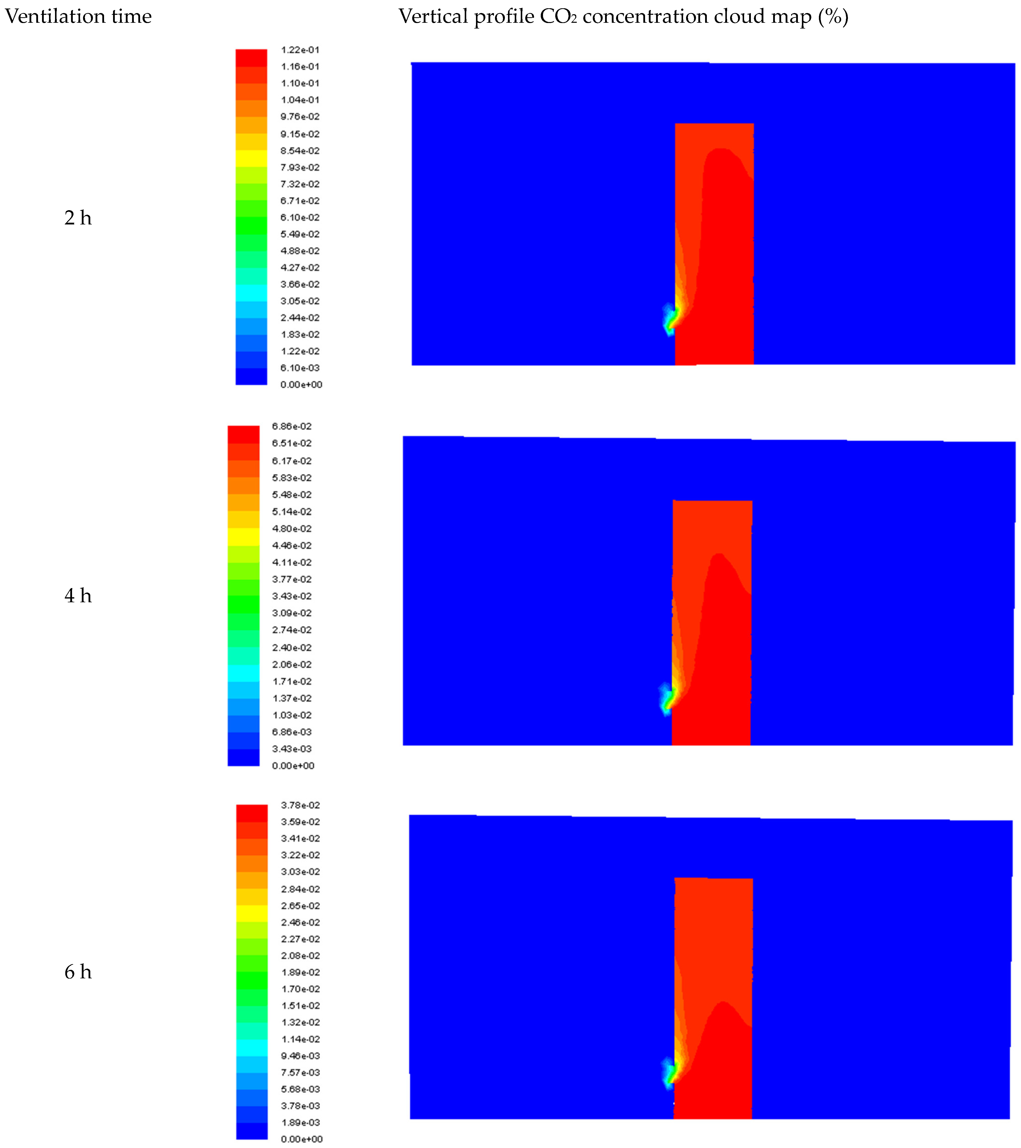
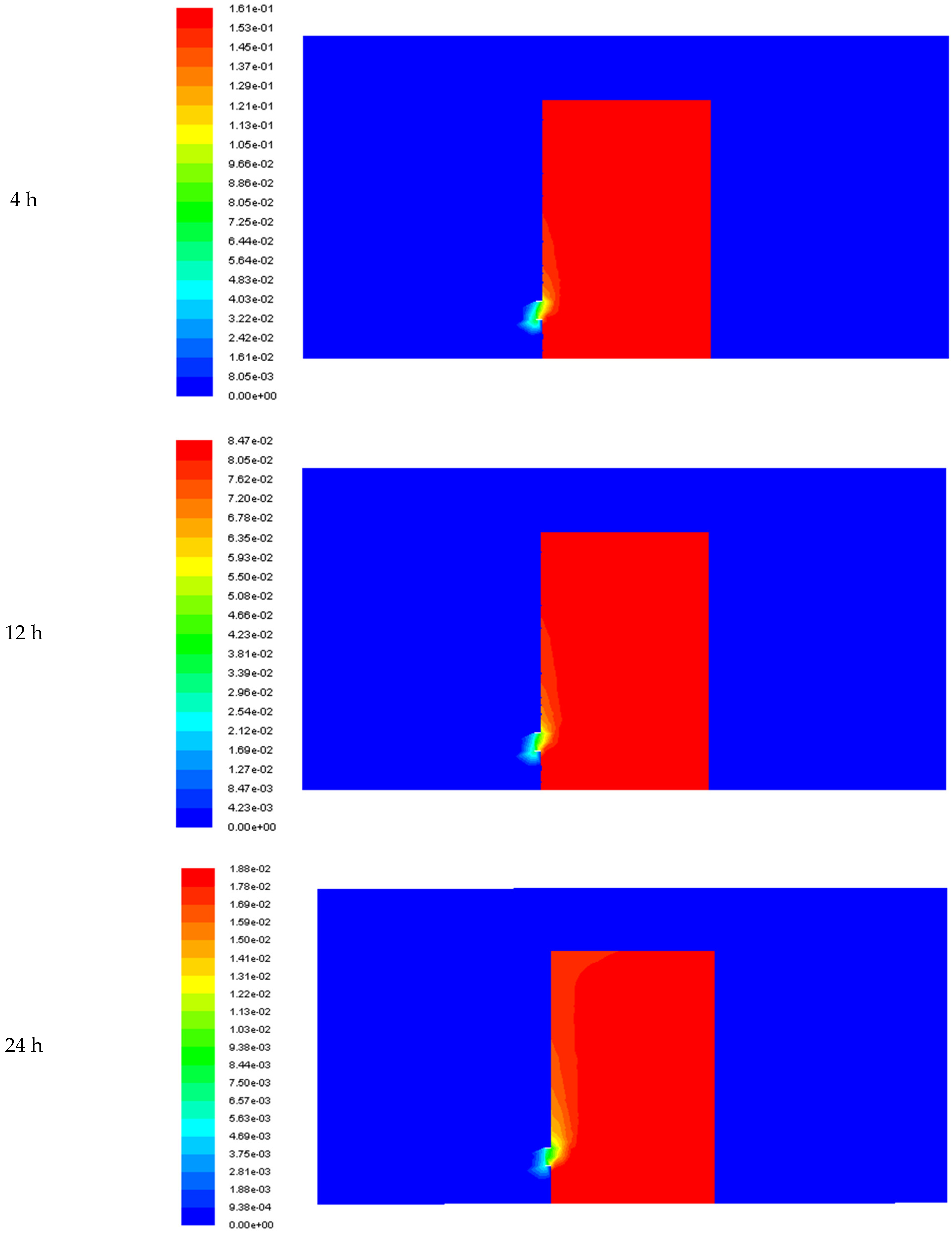
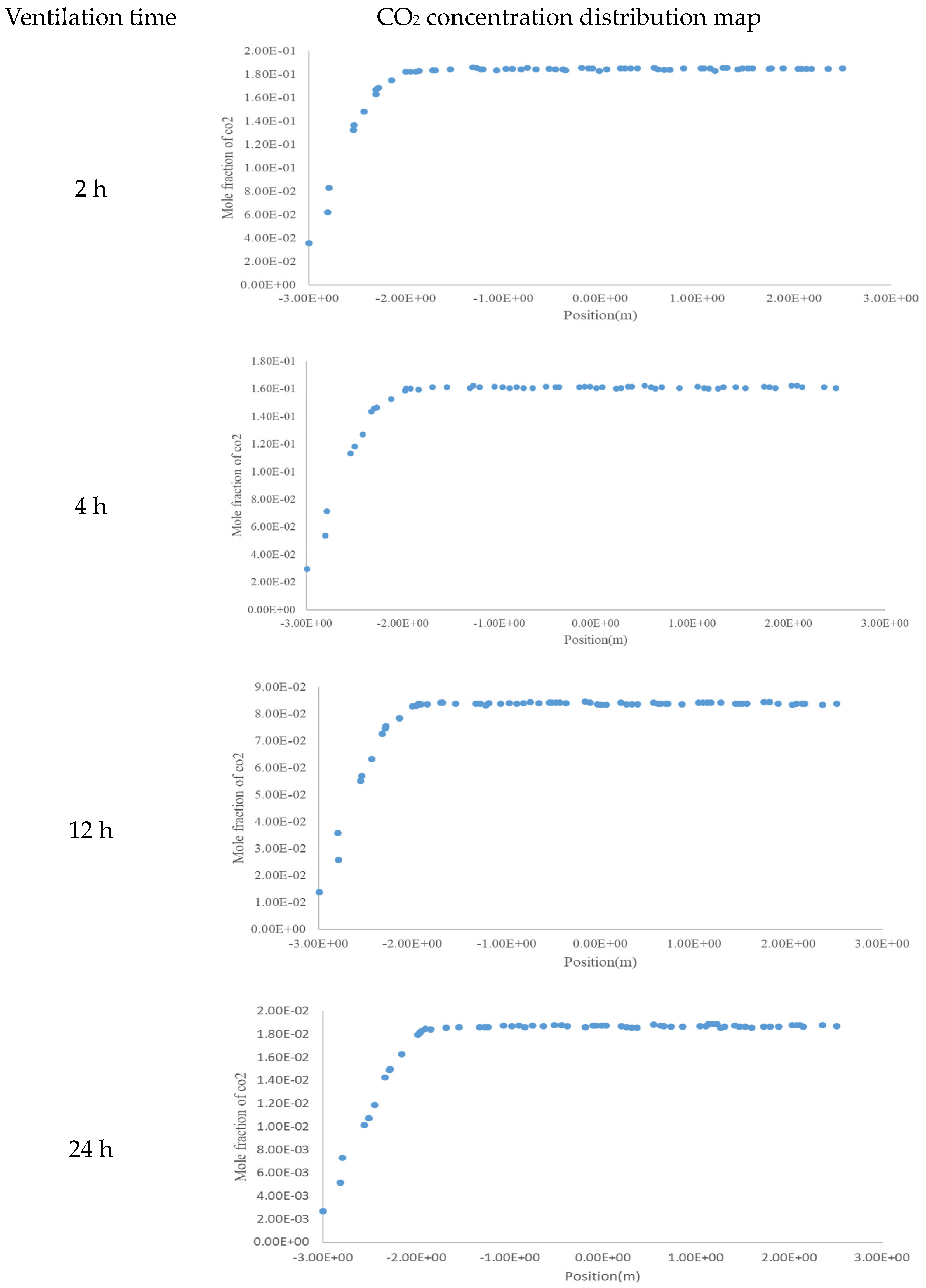
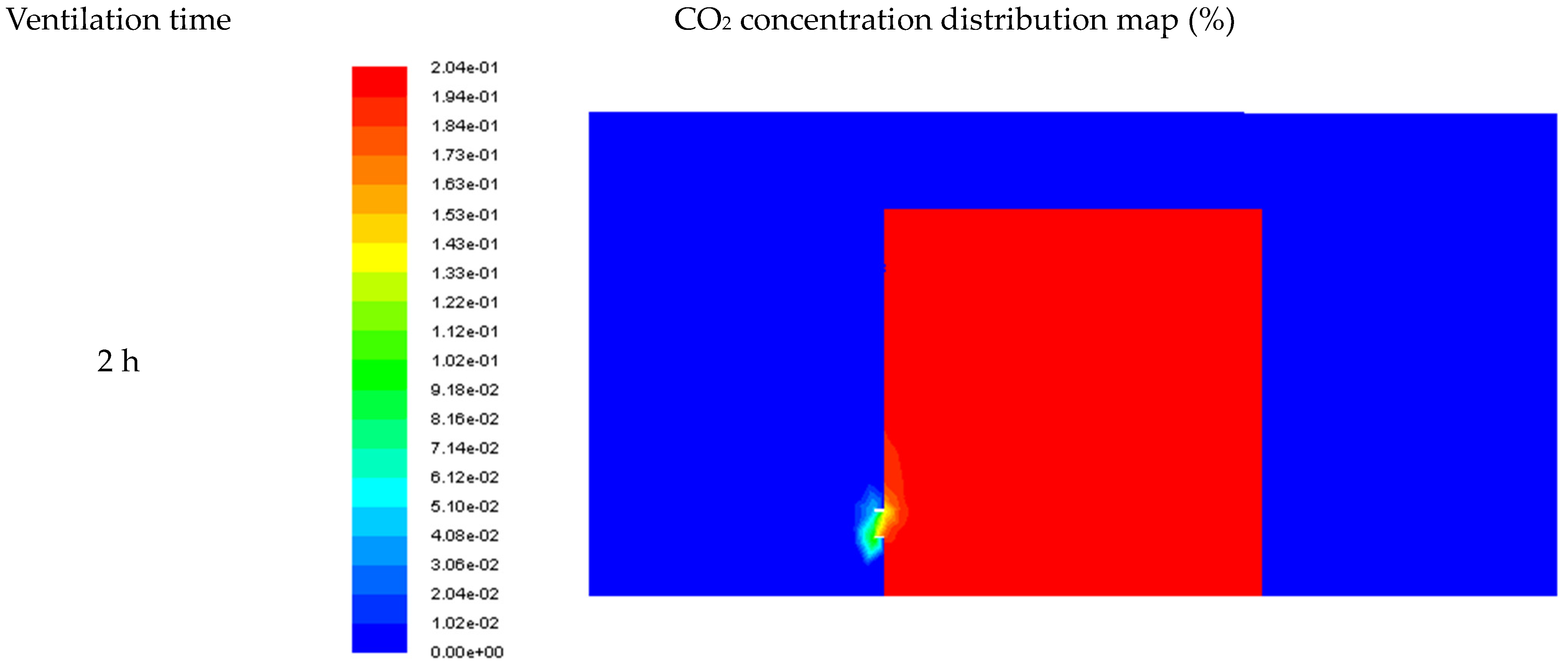
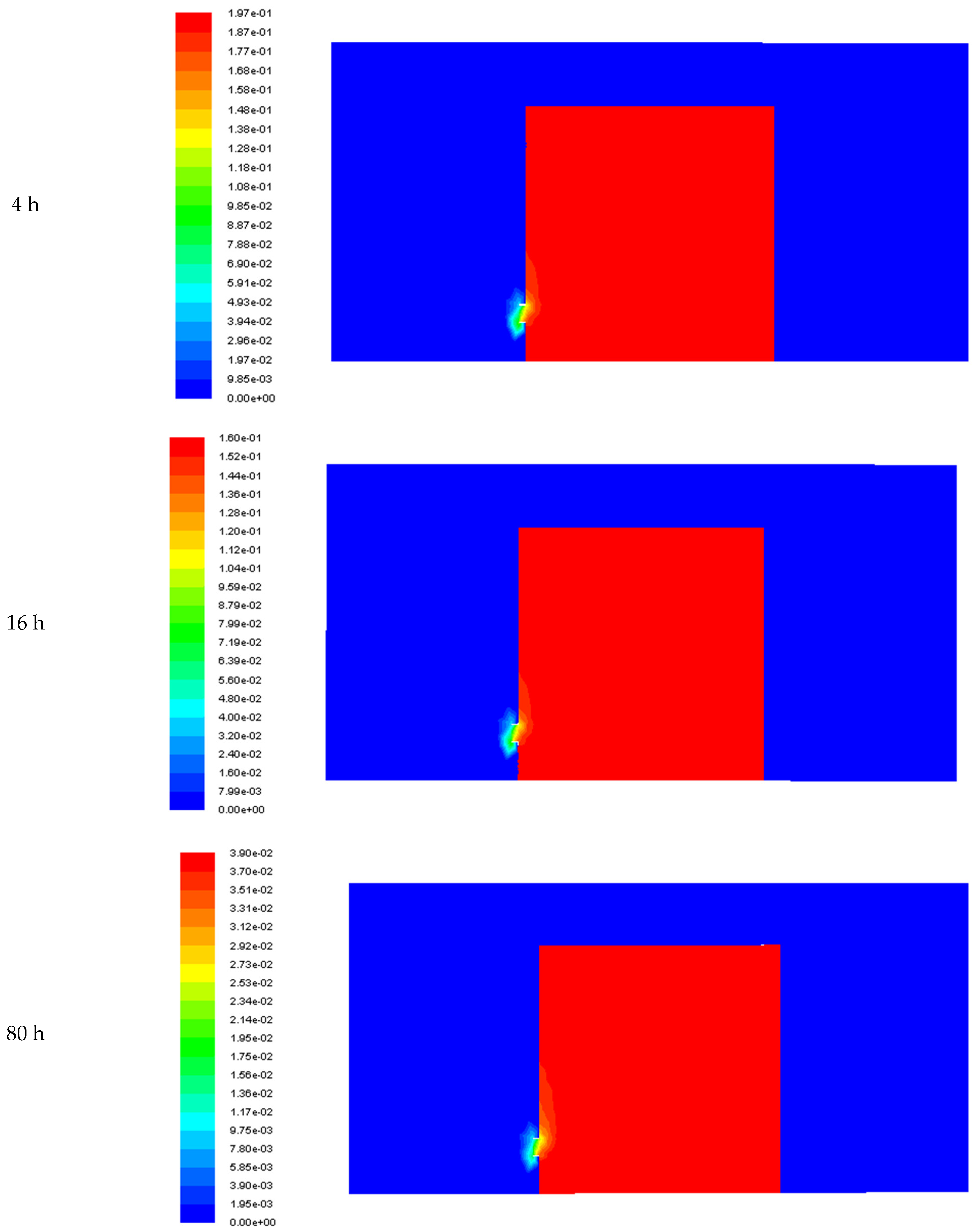
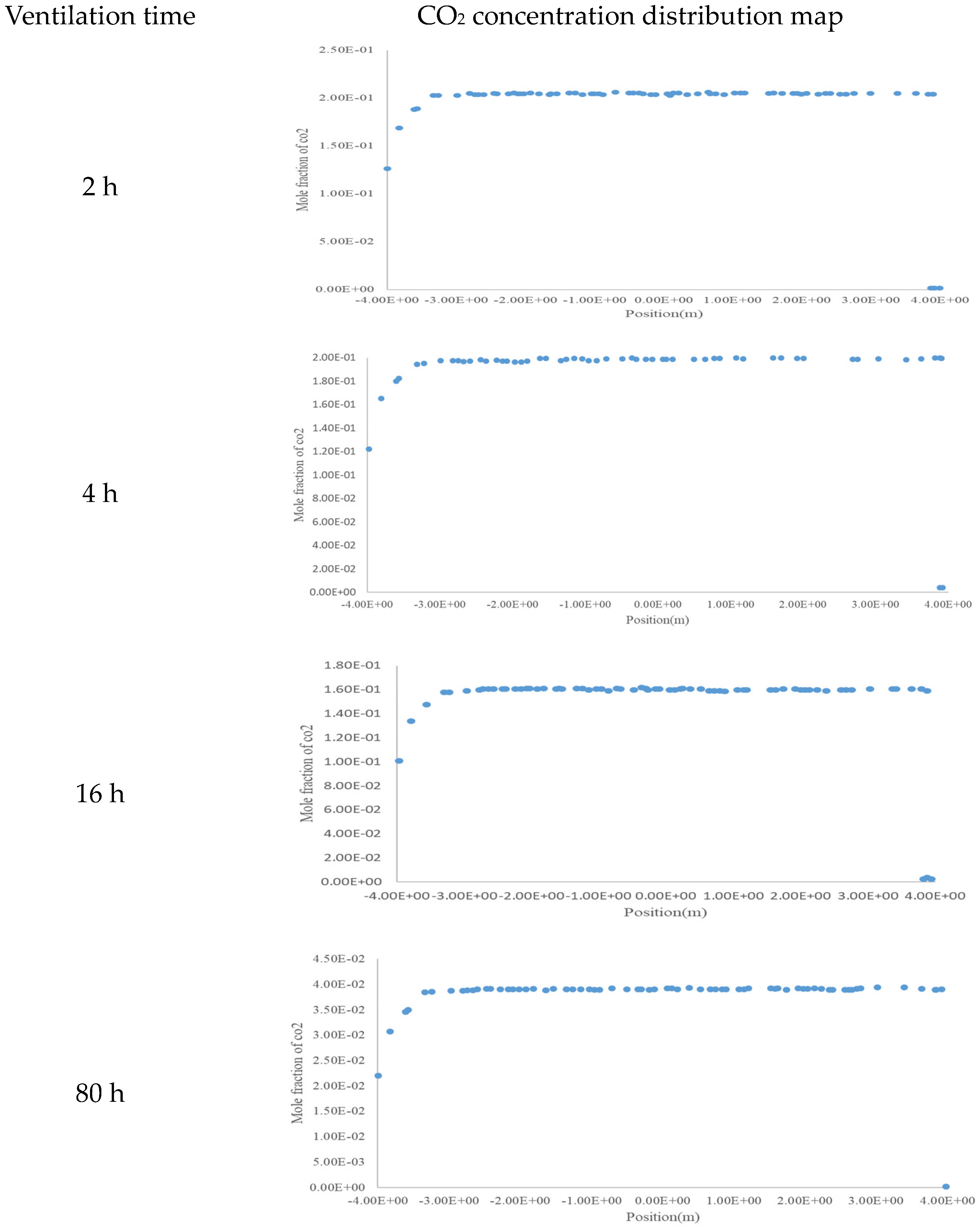
From the cloud diagram presented in Figure 3, it can be seen that under the condition of a low wind speed in natural ventilation, the gas flow field in manhole tank 1 was less affected by the external airflow, and only a small range of fluctuations in the flow field occurred near the manhole. The overall migration of CO2 was relatively slow, and it slowly diffused to the outside of the manhole. Figure 4 reflects the change in CO2 concentration along the respiratory belt height at different times; this height also corresponded with the center of the manhole opening. We observed that there was a gradient of the CO2 concentration in the online graph from the external environment to the inside of the tank at approximately 1 m around the manhole. At the beginning of ventilation, the CO2 content in the tank was maintained at approximately 21%. After 2 h of ventilation, the CO2 content in the tank decreased to approximately 12%—a significant decrease. After 4 h of ventilation, the CO2 content in the tank decreased to approximately 6.8%, and ventilation demonstrated significant effects. After 6 h of ventilation, the CO2 content in the tank decreased to approximately 3.75%, with an overall decrease of 18%. By analyzing the change in CO2 concentration at the height of the breathing belt in a vertical single-manhole gas tank, we concluded that under natural ventilation, it is necessary to ventilate a tank for longer than 6 h to discharge CO2 to a value of less than 2%.
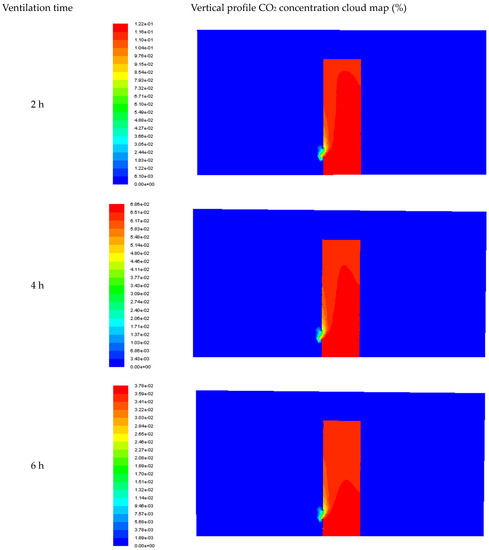
Figure 3.
Distribution program of CO2 concentrations in the longitudinal section of a tank body at different ventilation times.
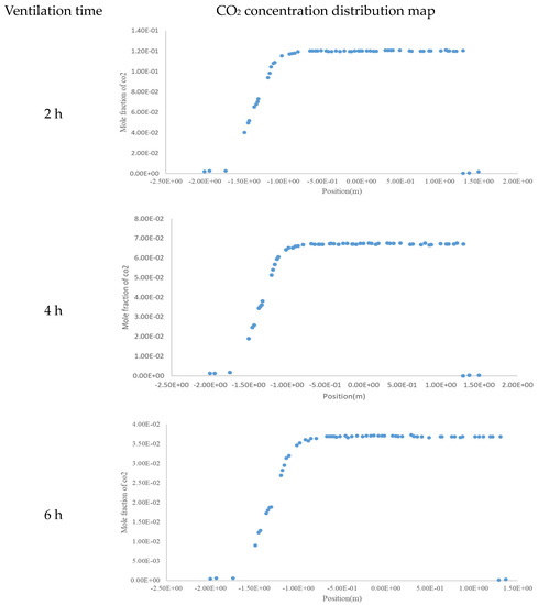
Figure 4.
CO2 concentration distribution diagrams at the height of the tank breathing zone at different ventilation times.
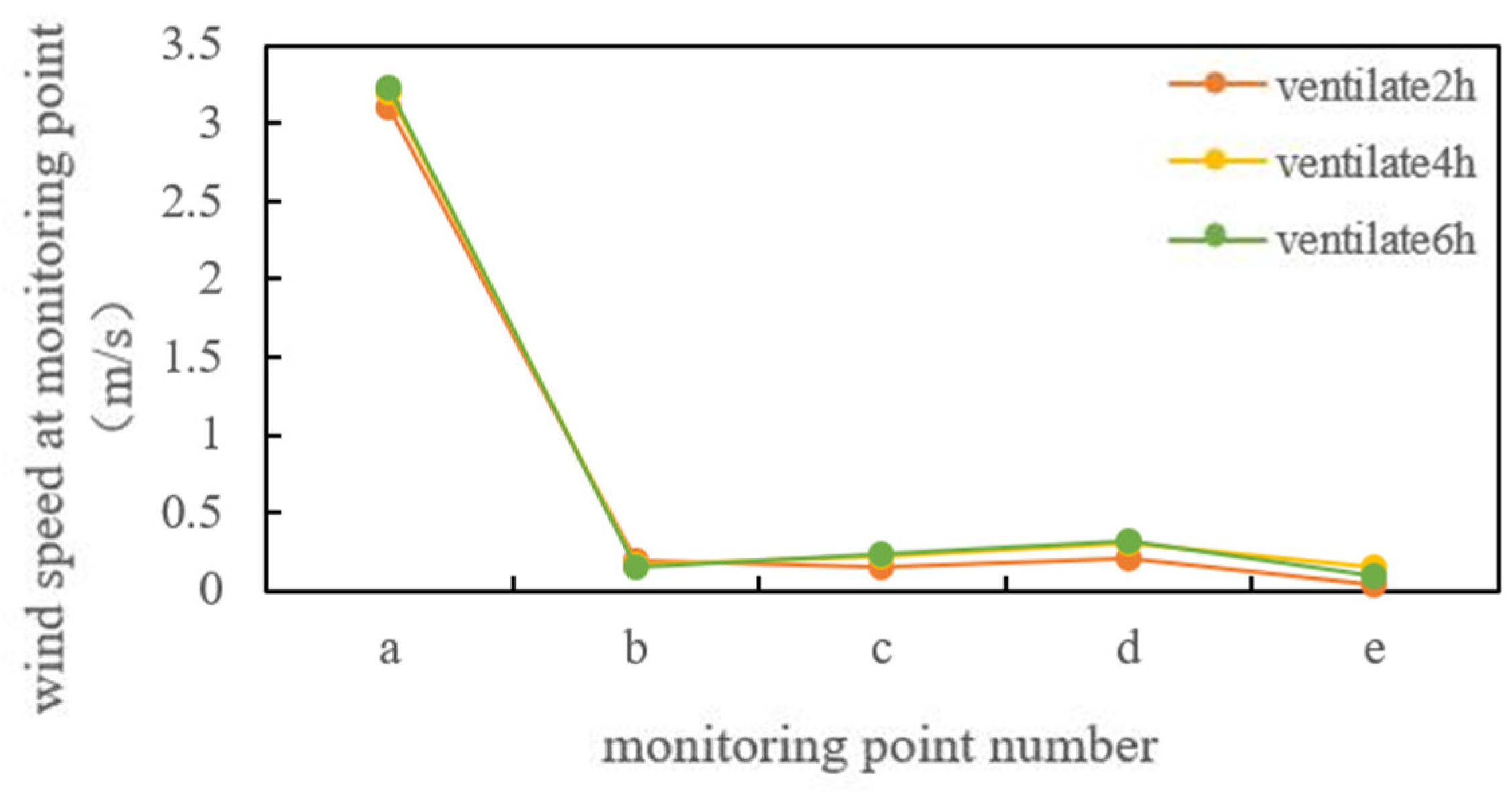
After processing the simulation results using FLUENT, the corresponding wind speeds at each detection point were obtained (Figure 5). Under this ventilation condition with no duct arrangement, the wind speed at each detection point significantly fluctuated. There was a maximum wind speed of 3.2 m/s at detection point a, whereas the wind speed at detection points b, c, d, and e fluctuated within the range of 0–0.5 m/s. The difference between the peak and minimum wind speeds at the detection point was significant and the distribution of wind speed in the tank was uneven. After entering the tank, fresh air was restricted to the area near the point opposite the air supply outlet. This area had good gas fluidity and a high wind speed, whereas the gas in the other areas had almost no flow. Under normal ventilation conditions, the distribution uniformity of the wind speed in the tank was not ideal, with the disadvantage of a dead corner area for air supply. Fresh air could not effectively flow into the tank, which was not conducive to diluting the toxic gas in the entire area of the tank.
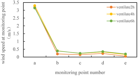
Figure 5.
Monitoring point wind speed of 2.6 m-diameter gas tank.
4.2. Simulation Results of Gas Migration in a Vertical, Single-Manhole, 5.2 m-Diameter Gas Tank
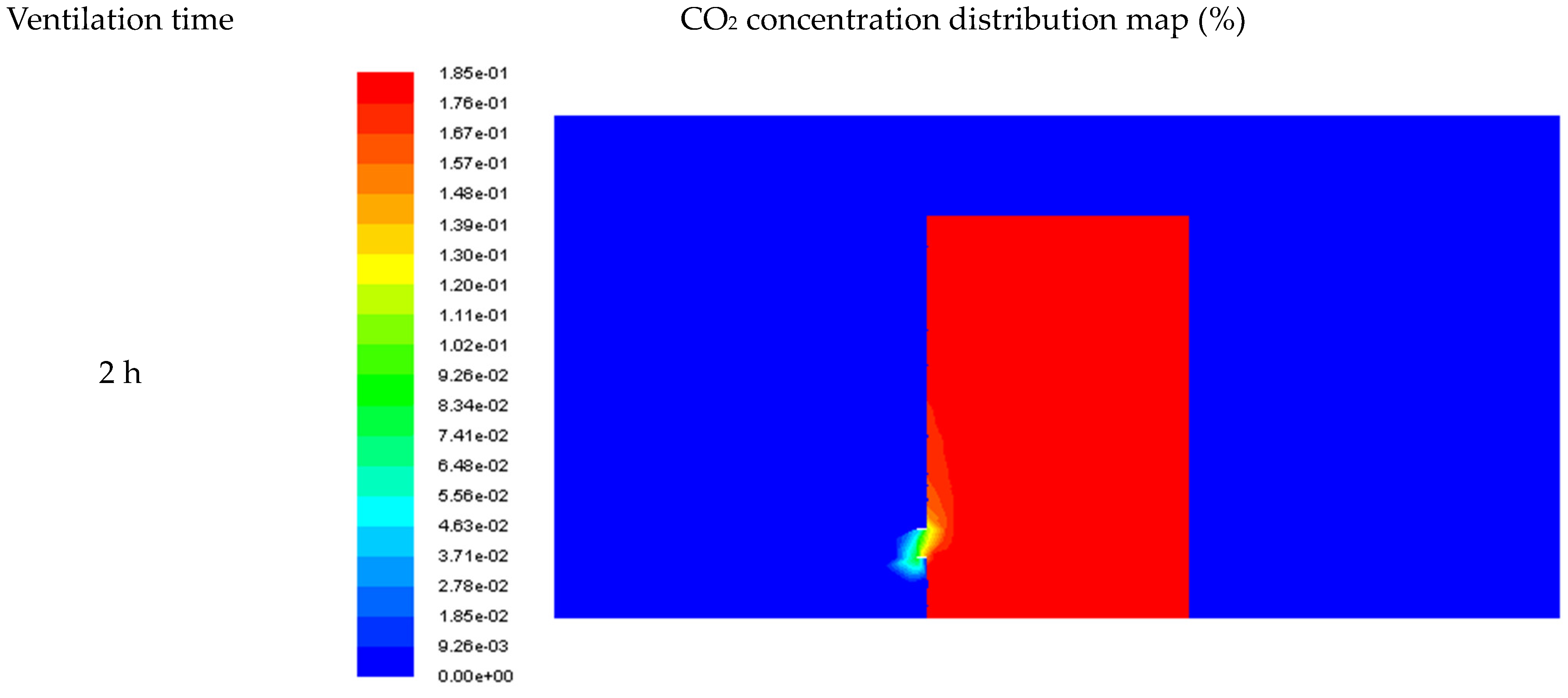
From the cloud diagram presented in Figure 6, it can be seen that under the condition of a low wind speed in natural ventilation, a single-manhole vertical tank with a bottom diameter of 5.2 m and a bottom diameter of 2.6 m had similar laws of influence on the gas flow field inside the tank by the external airflow, and the overall CO2 migration was slower. Figure 7 demonstrates that there was a gradient in the concentration of CO2 from the external environment to the inside of the tank approximately 1 m from the manhole. From the beginning of ventilation to 30 min, the CO2 content in the tank remained approximately 21%. After 2 h of ventilation, the CO2 content in the tank decreased to approximately 18.5%. After 4 h of ventilation, the CO2 content in the tank decreased to approximately 16%. After 6 h of ventilation, the CO2 content in the tank decreased noticeably to approximately 14%. After 12 h of ventilation, the CO2 content in the tank decreased to approximately 8.5%, and ventilation demonstrated significant effects. After 24 h of ventilation, the CO2 content in the tank decreased to below 2%.


Figure 6.
Distribution program of CO2 concentrations in the longitudinal section of a tank body at different ventilation times.

Figure 7.
CO2 concentration distribution diagrams at the height of the tank breathing zone at different ventilation times.
After processing the simulation results using FLUENT, the corresponding wind speeds of each detection point were obtained (Figure 8). Under this ventilation condition without a pipeline layout, the wind speed fluctuation amplitude of each detection point was relatively large. The maximum wind speed at detection point a was 3.1 m/s, whereas the wind speed at detection points b, c, d, and e fluctuated within the range of 0–0.5 m/s. The difference between the peak and minimum wind speeds at the detection point was significant and the distribution of wind speed inside the tank was uneven. After entering the tank, fresh air was restricted to the area near the point opposite the air supply outlet. This area had good gas fluidity and a high wind speed, whereas the gas in the other areas had almost no flow. Under normal ventilation conditions, the distribution uniformity of the wind speed in the tank was not ideal, with the disadvantage of a dead corner area for air supply. Fresh air could not effectively flow into the tank, which was not conducive to diluting the toxic gas in the entire area of the tank.
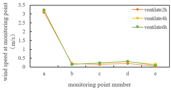
Figure 8.
Monitoring point wind speed of 5.2 m-diameter gas tank.
4.3. Simulation Results of Gas Migration in a Vertical, Single-Manhole, 7.8 m-Diameter Gas Tank
As can be seen from the cloud diagram in Figure 9, under the condition of a low wind speed in natural ventilation, the gas flow field in a single-manhole vertical tank with a bottom diameter of 7.8 m was hardly affected by the external airflow, and the overall migration of CO2 was extremely slow. In Figure 10, it can be observed that there was a gradient in the CO2 concentration from the external environment to the inside of the tank at approximately 0.5 m around the manhole, with a smaller gradient variation range compared with the other two sizes. After 2 h of ventilation, the CO2 content in the tank changed very little, maintaining a level of approximately 21%. After 4 h of ventilation, the CO2 content in the tank decreased to approximately 20%. After 16 h of ventilation, the CO2 content in the tank decreased to approximately 16%, a difference of only 4%. After 56 h of ventilation, the CO2 content in the tank decreased to approximately 7%, and the ventilation had a significant effect. Ultimately, under natural ventilation, it took longer than 80 h to ventilate the exhaust CO2 in the tank to less than 2%.


Figure 9.
Distribution program of CO2 concentrations in the longitudinal section of a tank body at different ventilation times.

Figure 10.
CO2 concentration distribution diagrams at the height of the tank breathing zone at different ventilation times.
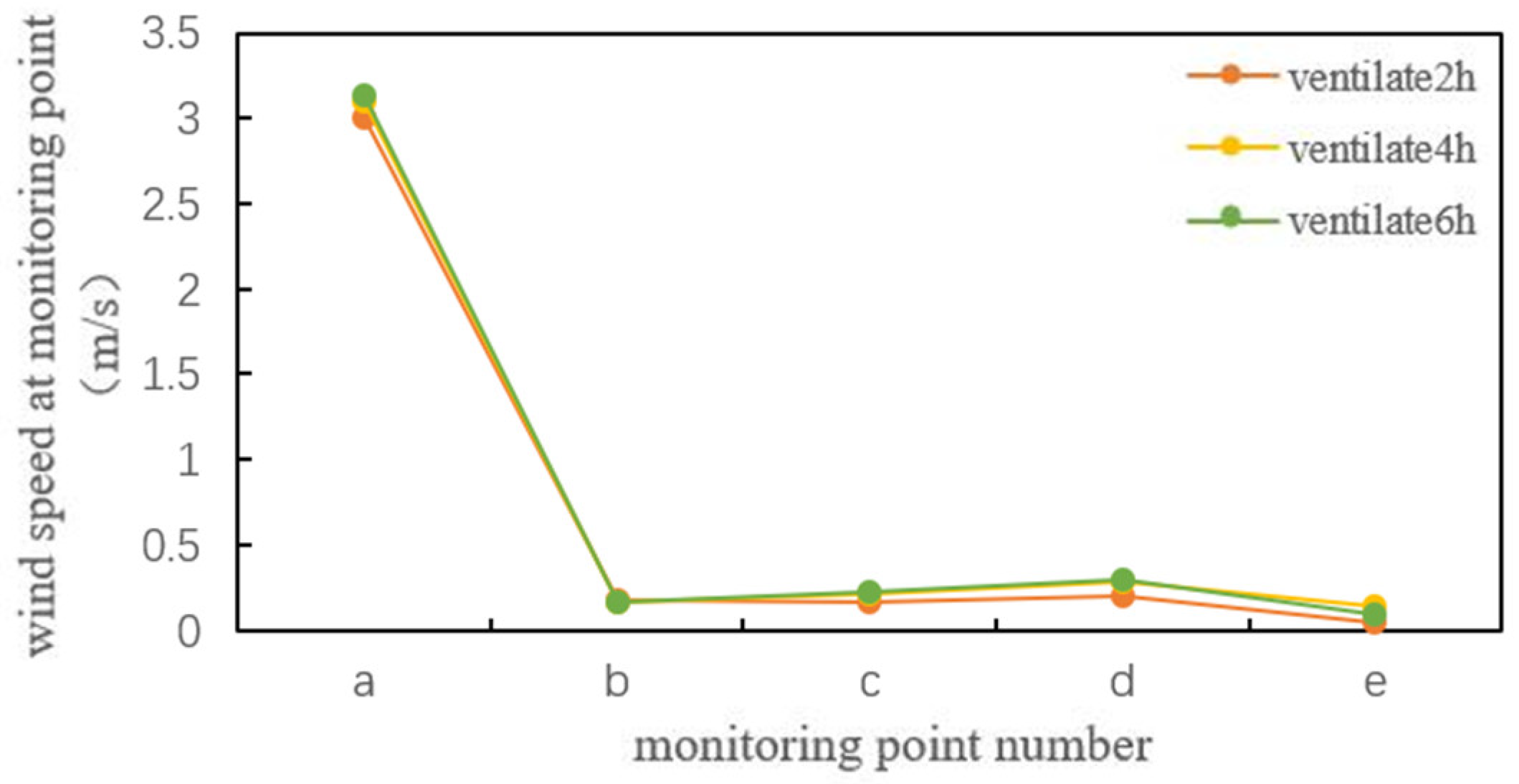
After processing the simulation results using FLUENT, the corresponding wind speeds at each detection point were obtained (Figure 11). Under this ventilation condition with no duct arrangement, the wind speed at each detection point significantly fluctuated. There was a maximum wind speed of 3 m/s at detection point a, whereas the wind speed at detection points b, c, d, and e fluctuated within the range of 0–0.5 m/s. The difference between the peak and minimum wind speeds at the detection points was significant and the distribution of wind speed in the tank was uneven. After entering the tank, fresh air was restricted to the area near the point opposite the air supply outlet. This area had good gas fluidity and a high wind speed, whereas the gas in the other areas had almost no flow. Under normal ventilation conditions, the distribution uniformity of the wind speed in the tank was not ideal, with the disadvantage of a dead corner area for air supply. Fresh air could not effectively flow into the tank, which was not conducive to diluting the toxic gas in the entire area of the tank.
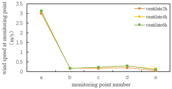
Figure 11.
Monitoring point wind speed of 7.8 m-diameter gas tank.
5. Risk Analysis of Gas Tank Operation
5.1. Theoretical Prediction Analysis
For the theoretical analysis of vertical tank ventilation, Warren [38] studied unilateral ventilation through a wind tunnel and summed up a relatively simple prediction method for unilateral opening ventilation [34]:
where qv is the ventilation volume (m3/s), U is the wind speed at the opening (m/s), and Aeff is the effective opening area (m2).
The effective opening area of the vertical tank in our study was the manhole area, and the calculated manhole area was 0.2826 m2. The wind speed at the manhole was 3 m/s. Therefore, the ventilation rate per second was 0.021195 m3/s, which was very low. The ventilation volume of the opening on one side was not completely equal to the ventilation volume; therefore, not all the gas entering the tank participated in the ventilation. Due to the narrowness of the manhole, a part of the air entered the tank and was then squeezed out of the tank [39,40,41]. Studies have shown that only approximately 37% of the gas is exchanged per hour [42]. At the beginning of ventilation, there was approximately 21% CO2 gas inside the tank. Therefore, through calculations, the hourly CO2 gas exchange volume was approximately 7% and, according to the formula, the ventilation volume was related to the manhole area. Theoretically, the hourly ventilation volume should not have had a particularly large fluctuation. In the actual simulation process, there was a certain deviation from the theoretical value due to the influence of factors such as the grid density in the early stage, the quality of the grid, the setting of the simulation parameters in the later stage, and changes in the actual wind speed and direction. When the diameter of the tank was 2.6 m, the exchange volume per hour was approximately 3%. With an increase in the simulation time, the decline range slightly reduced. When the diameter of the tank was 5.2 m, the exchange volume per hour was approximately 2.5%. With an increase in the simulation time, the decline range slightly decreased. When the tank diameter was 7.8 m, the exchange volume per hour was approximately 1%. With an increase in the simulation time, the decline range slightly decreased. As the air disturbance in the tank caused by natural ventilation decreased, the required ventilation time was longer and the drop was smaller; as the diameter of the tank increased, air disturbance in the tank was more difficult.
The gaseous density of CO2 is 1.997 g/L, which is higher than that of air. Therefore, CO2 easily accumulates in the lower part of a gas tank. According to the simulated cloud map, the diffusion of CO2 gas first decreased from the upper part of the gas tank and then gradually reduced. Therefore, according to our simulation results, when setting monitoring points in an actual process, at least one monitoring point should be set at the upper and lower ends of a gas tank, respectively. When the concentrations at the monitoring points of the upper and lower ends reach a safe range, they indicate that ventilation in the gas tank is completed from top to bottom. According to the “Safety Technical Specifications for Underground Confined Space Operation Part 2: Gas Detection and Ventilation”, the upper limit of the concentration of CO2 in a confined space should be 5400 mg/m3 and the density of CO2 should be 1.997 g/L; that is, 1997 mg/m3. The upper limit of the maximum concentration of CO2 is 36.98%; when working in a closed space due to a poor ventilation environment, the concentration of CO2 should be reduced to 1000 ppm before entering the workspace. According to our simulation, the tank diameter of 2.6 m required ventilation for at least 6 h, the tank diameter of 5.2 m required ventilation for at least 24 h, and the tank diameter of 7.8 m required ventilation for at least 80 h. Gas concentration monitoring is required and work should only commence after the monitoring reaches an acceptable standard.
5.2. Theoretical Prediction Analysis
Based on the above numerical simulation analysis of vertical storage tanks, we concluded that vertical storage tanks with a limited inlet and outlet have poor ventilation effects and take a significant amount of time to ventilate. This can lead to workers not effectively ventilating a tank before entering the tank for inspection and maintenance or other confined-space operations, resulting in excessive residual toxic gases in the internal space and a low oxygen content in the tank. This can result in the poisoning and suffocation of personnel. The research object used for ventilation experiments of hazardous chemical transportation tank cars is a large tank body with a length of approximately 13 m. If a 1:1 customized model is used for an experiment based on an actual tank car size, it is costly, and the laboratory space is limited. To ensure the reasonable use of resources and experimental conditions, models are usually constructed according to a reduced scale for experiments. Small-scale experiments are also safe and easy to control. Due to the limited resources and conditions of ventilation experiments [43], the required ventilation duration for similar tank bodies was derived to validate the effectiveness of the simulation. The main body of the ventilation experiment was a cylindrical tank, and the experimental material was composed of transparent acrylic material; thus, changes in the ventilation effect inside the tank were visually observed [43]. The tank model and the geometric dimensions of the ventilation duct were strictly reduced according to a model ratio rate of 1:8. The entire experimental platform constructed was mainly composed of three parts: the tank model, a fan, and a frequency converter.
The main goal of vertical tank ventilation is to quickly and efficiently dilute toxic gases in the tank, but ventilation can cause differences in the dilution degree of harmful gases in various areas within a tank. Therefore, an evaluation of the dilution effectiveness of harmful gases in a tank under different ventilation conditions should be conducted by comparing and analyzing the overall dilution efficiency and uniformity of the harmful gases in the tank for the same ventilation time. The higher the relative dilution rate, the more uniform the dilution degree and the better the ventilation effect [43]. We postprocessed a gas mass fraction monitoring dataset in FLUENT to obtain the residual harmful gas concentration (M1) in the tank after ventilation under corresponding working conditions. The parameter K was defined as the relative dilution ratio of harmful gases, indicating the degree of the relative reduction in the concentration of harmful gases in the tank after 100 s of ventilation. The larger the relative dilution ratio K, the faster the ventilation rate and the better the ventilation effect. The lower the K value, the slower the ventilation rate and the poorer the ventilation effect [43]. The calculation formula used was as follows [43]:
where M0 is the initial concentration of harmful gas and M1 is the residual concentration of harmful gas after ventilation.
We modified the formula and introduced parameter η to indicate the non-uniformity coefficient of the diluted gas in each area of the tank at the end of ventilation. The higher the value of non-uniformity coefficient η, the more uneven the degree of dilution of the gas. The smaller the value of non-uniformity coefficient η, the more uniform the degree of dilution of the gas. Parameters were introduced into each formula as θ. To correct the differences between horizontal and vertical storage tanks in the literature, the relevant formulas used were as follows [43]:
where is the reduction in harmful gases in various areas of the tank after ventilation, is the average concentration of the diluted harmful gas, n is the number of harmful gas concentration detection points, is the mean square deviation, η is the non-uniformity coefficient of the diluted harmful gas, and θ is the correction factor.
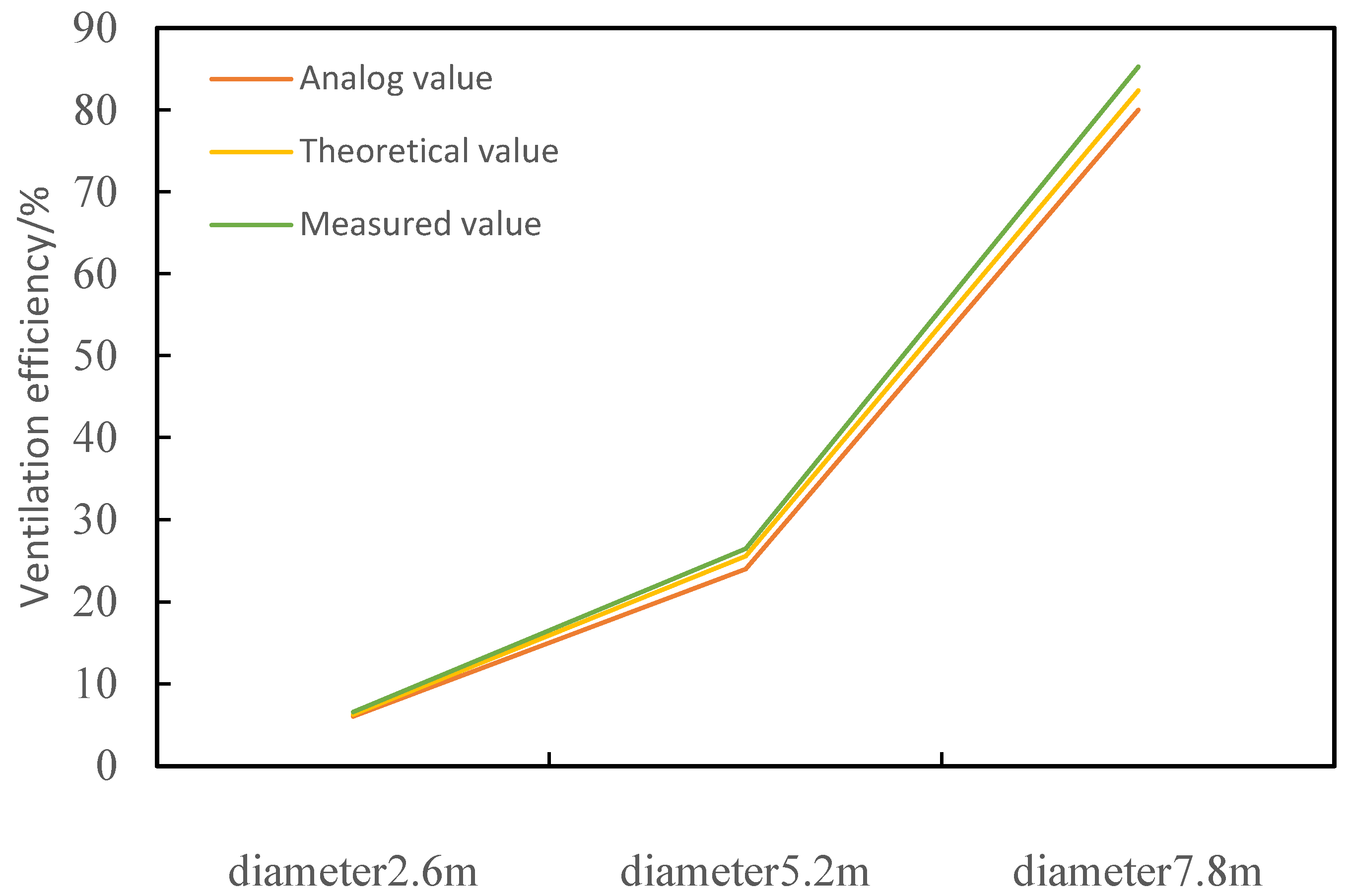
A numerical simulation was conducted for the normal ventilation mode of vertical tanks; that is, direct air supply at the manhole. The wind speed non-uniformity coefficient η under the basic working condition was calculated through postprocessing to be 2.45, the relative dilution ratio K of the ventilation gas was 23.8%, and the diluted non-uniformity coefficient η was 1.29. This indicated that under conventional ventilation conditions, there were drawbacks such as low ventilation efficiency and an uneven distribution; harmful gases were limited to one end of the tank body. We compared and analyzed the obtained simulation values with theoretical and experimental test values. The results are shown in Figure 12.

Figure 12.
Comparison of simulated, theoretical, and measured values.
By comparing the data, we observed that the variation trend between the simulated value and the theoretical value as well as the experimental test value were the same. The measured ventilation duration value was greater than the theoretical ventilation duration value, which was greater than the simulated ventilation duration value. When the diameter of the vertical tank was 2.6 m, the simulated time value was approximately 6 h, the theoretical value was approximately 6.27 h, and the measured value was approximately 6.59 h. When the diameter of the vertical tank was 5.2 m, the simulated value was approximately 24 h, the theoretical value was approximately 25.54 h, and the measured value was approximately 26.49 h. When the diameter of the vertical tank was 7.8 m, the simulated value was approximately 80 h, the theoretical value was approximately 82.39 h, and the measured value was approximately 85.27 h. Due to differences in the parameter settings and experimental environments during the simulation and experiment, there was a slight deviation in the ventilation results, but the overall trend was similar. Therefore, the simulation results and theoretical analysis could be used for a risk analysis of gas tanks.
We compared the experimental data with the simulation data and selected the parameter conditions that changed the ventilation speed for a comparative analysis. Under the same working conditions, the measured and simulated wind speed values at each detection point had the same trend of variation and the distribution characteristics of the wind speed were consistent. When the ventilation speed was 6 m/s, the maximum relative error between the simulated and measured values of the wind speed at each detection point was 12.71%, and the average relative error of the wind speed was 1.41%. When the ventilation speed was 8 m/s, the maximum relative error between the simulated and measured wind speeds at each detection point was 12.53%, and the average relative error of the wind speed was 1.62%. When the ventilation speed was 10 m/s, the maximum relative error between the simulated and measured wind speeds at each detection point was 11.45%, and the average relative error of the wind speed was 2.26%. When the ventilation speed was 12 m/s, the maximum relative error between the simulated and measured values of the wind speed at each detection point was 13.08%, and the average relative error of the wind speed was 6.01%. When the ventilation speed was 14 m/s, the maximum relative error between the simulated and measured values of the wind speed at each detection point was 9.03%, and the average relative error of the wind speed was 1.83% [43]. Although there were a few errors, they were within an acceptable range. This indicated that the ventilation result analysis was reliable and reasonable. The reason for the errors may have been because the numerical simulation was based on an ideal simplification. When collecting and recording experimental data, the data may have been influenced by the environment and relevant personnel as well as fluctuation values in the anemometer. There was an inevitable deviation between the placement of the detection equipment and the planned detection points during the experimental data collection, whereas the numerical simulation values were obtained at precise points within the calculation model. This may also have led to errors between the simulated values and the on-site measured values.
6. Discussion
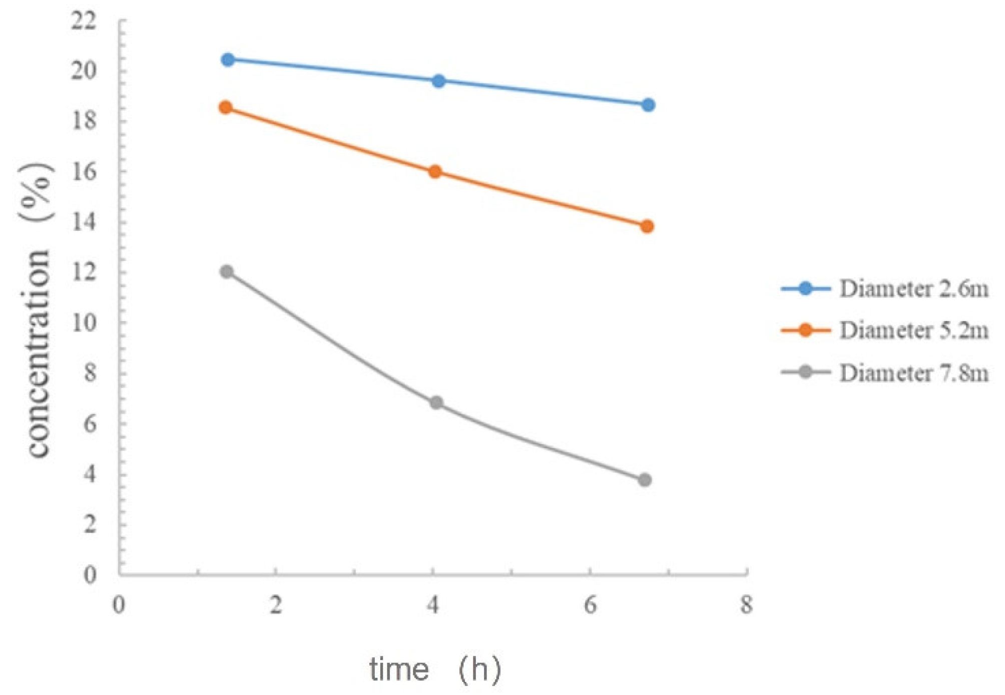
Through the numerical simulation of the ventilation effect of vertical tanks with different diameters, we studied the transport characteristics of CO2 gas in gas tanks under natural ventilation conditions. The results demonstrated that (1) in the case of different tank diameters, the larger the diameter, the lesser the air disturbance caused by external wind to the inside of the tank and the longer the required ventilation time; and (2) according to the cloud diagram of the simulation results, at least one monitoring point should be set at the upper and lower ends of a gas tank, respectively, for a vertical tank. Figure 13 shows the changes in CO2 concentrations at different times at the center point of the horizontal line at the height of the breathing zone in the three single-manhole vertical gas tanks with different tank diameters.

Figure 13.
The results of CO2 concentration changes under different tank diameters.
The time required for the natural ventilation of a manhole air tank under the three diameters was relatively long. When the number of manholes was the same, the ventilation time increased with an increase in the diameter of the tank. If the natural ventilation of a manhole did not disturb the gas inside the tank, the ventilation time increased with an increase in the diameter of the tank.
It is, therefore, not possible to solely rely on natural ventilation when operating in a confined space in larger tank equipment because the flow field in a single-hole tank is not easily disturbed; thus, the longer the operation time, the worse the air quality in the tank [44]. After ventilation, operational procedures must be strictly followed. Regulations are required prohibiting long-term operation or interval ventilation to ensure that the air quality in a tank is acceptable. The distribution of CO2 gas in a gas tank is relatively uniform; when entering a tank with sufficient natural ventilation and if the operator monitors the surrounding gas concentration and finds it to be acceptable, the gas concentration in the tank is basically within an acceptable range.
In a simulation process, there are many shortcomings: the division of the grid in the early stage of the simulation affects the simulation results at a later stage and in the actual process; and the type of gas tank, number of manholes, and gas present in the gas tank are different. The categories considered were not complete enough. In follow-up research, the influence of different grid divisions on the simulation results will be strengthened and the types of simulated gas tanks will be more comprehensive. If conditions permit, numerical simulation and field experiments will be used to ensure the ventilation results are more accurate. Although the influence of factors such as the wind speed and direction were considered as much as possible in the selection of numerical simulation conditions in this paper, certain errors remained. The reasons for the errors were as follows: (1) the wind direction and wind speed change under actual natural ventilation conditions; (2) generally speaking, the wind has a certain inclination angle relative to the horizontal direction, and the general variation range of the wind inclination angle is −10°~+10° [44]; (3) during a numerical simulation process, simulation results will vary, theoretically speaking [45], when the boundary conditions are set correctly. Thus, the higher the element order, the greater the mesh density and the more accurate the calculation results; however, the time cost is greater and more computer resources are required [46]. A simulation also provides a theoretical basis for the ventilation duration of different types of gas tanks. Through a cloud map of CO2 migration inside a tank, it is easier to identify the location where the local concentration is too high, reducing the risk for staff who enter the gas tank for operational procedures. This has practical significance. In subsequent research, the tank type and ventilation will be perfected and the theoretical basis for different types of gas tank ventilation will be provided.
7. Conclusions
- (1)
- We simulated gas tanks with tank diameters of 2.6 m, 5.2 m, and 7.8 m. The larger the diameter, the longer the required ventilation time. According to the simulation, the tank diameter of 2.6 m required ventilation for at least 6 h, the tank diameter of 5.2 m required ventilation for at least 24 h, and the tank diameter of 7.8 m required ventilation for at least 80 h. Therefore, gas concentration monitoring is required and work can commence after monitoring reaches the required standard.
- (2)
- The simulation results were compared with theoretical formula calculations and experimental test results. According to the calculation results, the hourly CO2 gas exchange was 7%. According to the simulation results, when the tank diameter was 2.6 m, the exchange rate per hour was approximately 3%, slightly decreasing with the increase in simulation time. When the tank diameter was 5.2 m, the exchange rate per hour was approximately 2.5%, slightly decreasing with the increase in simulation time. When the diameter of the tank was 7.8 m, the exchange rate per hour was approximately 1%, slightly decreasing with the increase in simulation time. The variation trend of the simulated value was the same as that of the theoretical value and the experimental test value. The measured value of the ventilation duration was greater than the theoretical value of the ventilation duration and this was greater than the simulated value of the ventilation duration. The larger the tank diameter, the longer the required ventilation time.
- (3)
- To ensure the safety of the working environment and the operators, a certain number of monitoring points are required for poorly ventilated gas tanks. According to the simulation results, at least one monitoring point should be set at the upper and lower ends of the gas tank, respectively, for a vertical tank. The monitoring results of the upper end and the lower end should all be verified, indicating that the overall ventilation of the gas tank is complete and that work can commence.
Author Contributions
Conceptualization, C.Y.; Methodology, Y.L. and X.L.; Software, Y.W.; Funding acquisition, C.Y. and X.L. All authors have read and agreed to the published version of the manuscript.
Funding
This study was financially supported by Innovation Engineering of Beijing Academy of Science and Technology (23CA001-04), the National Natural Science Foundation of China (52274245), the Opening Project of the State Key Laboratory of Explosion Science and Technology (Beijing Institute of Technology, KFJJ22-15M), Fundamental Research Funds for the Central Universities (2009QZ09), and the Youth Foundation of Social Science and Humanity Ministry of Education of China (19YJCZH087).
Data Availability Statement
Not applicable.
Conflicts of Interest
The authors declare no conflict of interest.
References
- Jiang, H. Analysis of Toxic and Hazardous Substances Before Working in Confined Spaces. Res. Contemp. Chem. Ind. 2020, 119–120. [Google Scholar]
- Dai, L.; Han, Y.; Wei, R.; Wang, G.; Song, W.; Xiang, J. Design of ventilation scheme for confined spaces. China Shipbuild. 2012, 53, 520–525. [Google Scholar]
- Li, X. Ventilation method for oil tank maintenance project. Pet. Eng. Constr. 2004, 20, 13–15+3. [Google Scholar]
- Li, Q.; Pan, C.; Li, X.; Wang, C. Methane leakage simulation in confined space. J. Bengbu Univ. 2022, 11, 26–28+35. [Google Scholar]
- Tan, C.; Liu, Y.; Wang, T.; Qin, Y. Numerical simulation of ventilation and protection technology for confined space in municipal heating. J. Harbin Inst. Technol. 2017, 49, 123–128. [Google Scholar]
- Yang, X.; Li, H.; Liu, H.; Chen, S. Three-dimensional numerical simulation analysis of gas flow field distribution and optimization in single-hole pressure vessel. Energy Conserv. 2019, 38, 61–64. [Google Scholar]
- Yang, C.; Liu, Y.; Qin, Y. Research on natural ventilation characteristics and influencing factors of single-opening confined space. Saf. Environ. Eng. 2019, 26, 183–189. [Google Scholar]
- Li, G. Safety simulation analysis of hazardous gas replacement in confined space. China Public Secur. (Acad. Ed.) 2015, 50–55. [Google Scholar] [CrossRef]
- Chen, Y.; Zhong, H.; Gao, H.; Zhang, Z. Research on air distribution simulation and thermal comfort under different ventilation conditions. Sci. Technol. Innov. 2020, 28–30. [Google Scholar]
- Li, Y. Numerical Simulation of Natural Gas Leakage, Diffusion, and Explosion in Confined Space; Capital University of Economics and Business: Beijing, China, 2011. [Google Scholar]
- Wang, Z. Numerical Simulation and Analysis of Gas Diffusion in Confined Space; Dalian University of Technology: Dalian, China, 2009. [Google Scholar]
- Li, X. Safety Analysis and Preventive Measures of Storage Tank Leakage in Liquefied Gas Filling Station; Chongqing Institute of Science and Technology: Chongqing, China, 2018. [Google Scholar]
- Quan, M.; Wang, Y.; Zhou, Y.; Xu, K.; Cao, Y.; Ren, X. Effect of swirl ventilation on contaminant removal in a cylindrical confined space. Build. Environ. 2021, 205, 108277. [Google Scholar] [CrossRef]
- Pouzou, J.G.; Chris, W.; Neitzel, R.L.; Croteau, G.A.; Yost, M.G.; Seixas, N.S. Confined space ventilation by shipyard welders: Observed use and effectiveness. Ann. Occup. Hyg. 2015, 59, 116–121. [Google Scholar]
- Zhao, W.; Zhang, T.; Jia, C.; Li, X.; Wu, K.; He, M. Numerical Simulation on Natural Gas Migration and Accumulation in Sweet Spots of Tight Reservoir. J. Nat. Gas Sci. Eng. 2020, 81, 103454. [Google Scholar] [CrossRef]
- Wei, S.Y.; Chen, X.X.; Dong, L.H.; Li, Z. Numerical Simulation Research of Gas Migration Laws on Real Underground Mining Conditions. In Mechanical Engineering and Control Systems: Proceedings of 2015 International Conference on Mechanical Engineering and Control Systems (MECS2015); World Scientific: London, UK, 2016. [Google Scholar]
- Lu, Q.; Wei, X.; Maoqing, B.E. Lattice Boltzmann Simulations of Gas Migration Law in Two-Dimension Goaf of Fully Mechanized Coal Caving Mining Face. In Proceedings of the International Conference on Computer Science Education, Kaifeng, China, 25–27 July 2008. [Google Scholar]
- Schmidt, D.; Krause, U.; Schmidtchen, U. Numerical simulation of hydrogen gas releases between buildings. Int. J. Hydrogen Energy 2008, 24, 479–488. [Google Scholar] [CrossRef]
- And, S.S.; Rigas, F. Fuel Gas Dispersion under Cryogenic Release Conditions. Energy Fuels 2005, 19, 2535–2544. [Google Scholar]
- Tauseef, S.M.; Rashtchian, D.; Abbasi, S.A. CFD-based simulation of dense gas dispersion in the presence of obstacles. J. Loss Prev. Process Ind. 2011, 24, 371–376. [Google Scholar] [CrossRef]
- Wang, Y. Research on Dynamic Risk Assessment and Emergency Response of Road Transport Accidents of Dangerous Chemicals; Beijing Institute of Petrochemical Technology: Beijing, China, 2021. [Google Scholar]
- Meel, A.; O’Neill, L.M.; Levin, J.H.; Seider, W.D.; Oktem, U.; Keren, N. Operational risk assessment of chemical industries by exploiting accident databases. J. Loss Prev. Process Ind. 2007, 20, 113–127. [Google Scholar] [CrossRef]
- Paltrinieri, N.; Khan, F.; Amyotte, P.; Cozzani, V. A dynamic approach to risk management: Application to the Hoeganaes metal dust accidents. Process Saf. Environ. Prot. 2014, 92, 669–679. [Google Scholar] [CrossRef]
- Kalantarnia, M.; Khan, F.; Hawboldt, K. Modelling of BP Texas City refinery accident using dynamic risk assessment approach. Process. Saf. Environ. Prot. 2010, 88, 191–199. [Google Scholar] [CrossRef]
- Rathnayaka, S.; Khan, F.; Amyotte, P. Accident modeling approach for safety assessment in an LNG processing facility. J. Loss Prev. Process Ind. 2012, 25, 414–423. [Google Scholar] [CrossRef]
- Wu, W. Structural Analysis and Safety Evaluation of Large Vertical Storage Tanks; Liaoning University of Petrochemical Technology: Fushun, China, 2020. [Google Scholar]
- Hu, Y. Theoretical Calculation and Numerical Simulation of Single Opening Natural Ventilation Driven by Unsteady Wind Pressure; Hunan University: Changsha, China, 2013. [Google Scholar]
- Wan, Y.; Li, L.; Wang, W.; Liang, P.; Huang, Y.; Chen, Z. Research on the leakage and diffusion law of LPG storage tanks based on Fluent’s wind direction. Pet. Nat. Gas Chem. Ind. 2021, 50, 98–103. [Google Scholar]
- Gonin, R.; Hogue, P.; Guibert, R.; Fabre, D.; Bourguet, R.; Ammouri, F.; Vyazmina, E. A computational fluid dynamic study of the filling of a gaseous hydrogen tank under two contrasted scenarios. Int. J. Hydrogen Energy 2022, 47, 23278–23292. [Google Scholar]
- Tao, J.; Li, Z.; Guo, Z.; Zhang, N. Calculation of LNG leakage gas concentration and temperature diffusion process. Cryog. Supercond. 2020, 48, 12–19+25. [Google Scholar]
- Zhang, J.; Xu, C.; An, J.; Yuan, Y. Numerical simulation of heavy air leakage and diffusion in rooms under different ventilation forms. Gas Heat 2018, 38, 32–38. [Google Scholar]
- Fu, W. Simulation and Experimental Research on Large Openings for Natural Ventilation; Xi’an University of Architecture and Technology: Xi’an, China, 2008. [Google Scholar]
- Ouellette, P.; Hill, P.G. Turbulent transient gas injections. J. Fluid Eng. 2000, 122, 743e52. [Google Scholar] [CrossRef]
- Galassi, M.C.; Baraldi, D.; Acosta Iborra, B.; Moretto, P. CFD analysis of fast filling scenarios for 70 MPa hydrogen type IV tanks. Int. J. Hydrogen Energy 2012, 37, 6886e92. [Google Scholar] [CrossRef]
- Galassi, M.C.; Papanikolaou, E.; Heitsch, M.; Baraldi, D.; Iborra, B.A.; Moretto, P. Assessment of CFD models for hydrogen fast filling simulations. Int. J. Hydrogen Energy 2014, 39, 6252e60. [Google Scholar]
- Melito, D.; Baraldi, D.; Galassi, M.C.; Ortiz Cebolla, R.; Acosta Iborra, B.; Moretto, P. CFD model performance benchmark of fast filling simulations of hydrogen tanks with pre-cooling. Int. J. Hydrogen Energy 2014, 39, 4389e95. [Google Scholar]
- Zhang, S.; Hong, B.; Gao, H. Grid ruler for numerical simulation of air and underwater blast shock waves Comparative analysis of inch effect. J. Hydraul. Eng. 2015, 46, 298–306. [Google Scholar]
- Hoogendoorn, C.J.; Afgan, N. Energy Conservation in Heating, Cooling, and Ventilating Buildings: Heat and Mass Transfer Techniques; Hemisphere Publishing Corporation: London, UK, 1978. [Google Scholar]
- Zhao, T. Numerical Study of Pollutant Diffusion in Adjacent Industrial Plants under Natural Ventilation; Xi’an University of Architecture and Technology: Xi’an, China, 2021. [Google Scholar]
- Xiong, Y. The Influence of the Concave and Convex Features of High-Rise Residential Planes on Unilateral Ventilation and Pollutant Concentration; Huazhong University of Science and Technology: Wuhan, China, 2021. [Google Scholar]
- Cai, L. Optimal Design of Natural Ventilation for Intermediate Units in High-Rise Residential Buildings; China University of Mining and Technology: Xuzhou, China, 2021. [Google Scholar]
- Zhang, H.; Li, W.; He, G.; Wang, M. Research on ventilation characteristics of rooms with one side opening. Chin. Foreign Archit. 2011, 116–117. [Google Scholar]
- Zhang, F. Research on the Optimization of Gas flow and Ventilation Inside Hazardous Chemical Transportation Tank Cars; China University of Mining and Technology: Xuzhou, China, 2022. [Google Scholar]
- Yang, Y. Study on Flue Gas Flow of Natural Exhaust Vents under the Action of Environmental Wind; Central South University: Changsha, China, 2011. [Google Scholar]
- Luo, J.; Zhou, X. Study on the influence of grid element shape on calculation accuracy in numerical simulation. J. Yellow River Univ. Sci. Technol. 2022, 24, 8–11. [Google Scholar]
- Xie, Z.; Han, Y. Research on the grid-scale effect of finite element analysis of temperature field. China Water Transp. (Second. Half Mon.) 2017, 17, 204–206. [Google Scholar]


Disclaimer/Publisher’s Note: The statements, opinions and data contained in all publications are solely those of the individual author(s) and contributor(s) and not of MDPI and/or the editor(s). MDPI and/or the editor(s) disclaim responsibility for any injury to people or property resulting from any ideas, methods, instructions or products referred to in the content. |
© 2023 by the authors. Licensee MDPI, Basel, Switzerland. This article is an open access article distributed under the terms and conditions of the Creative Commons Attribution (CC BY) license (https://creativecommons.org/licenses/by/4.0/).