Anomaly Detection for Wind Turbines Using Long Short-Term Memory-Based Variational Autoencoder Wasserstein Generation Adversarial Network under Semi-Supervised Training

Abstract

Intelligent anomaly detection for wind turbines using deep-learning methods has been extensively researched and yielded significant results. However, supervised learning necessitates sufficient labeled data to establish the discriminant boundary, while unsupervised learning lacks prior knowledge and heavily relies on assumptions about the distribution of anomalies. A long short-term memory-based variational autoencoder Wasserstein generation adversarial network (LSTM-based VAE-WGAN) was established in this paper to address the challenge of small and noisy wind turbine datasets. The VAE was utilized as the generator, with LSTM units replacing hidden layer neurons to effectively extract spatiotemporal factors. The similarity between the model-fit distribution and true distribution was quantified using Wasserstein distance, enabling complex high-dimensional data distributions to be learned. To enhance the performance and robustness of the proposed model, a two-stage adversarial semi-supervised training approach was implemented. Subsequently, a monitoring indicator based on reconstruction error was defined, with the threshold set at a 99.7% confidence interval for the distribution curve fitted by kernel density estimation (KDE). Real cases from a wind farm in northeast China have confirmed the feasibility and advancement of the proposed model, while also discussing the effects of various applied parameters.

1. Introduction

In response to the global energy shortage and climate deterioration following the Paris Agreement, renewables have attracted increasing attention in the past decade [1]. The rapid growth of wind power as a renewable energy source renders it strategically significant in expediting the transition towards green and low-carbon energy structures. The latest statistics from GWEC reveal that a cumulative wind-power capacity of 77.6 GW was successfully integrated into power grids in 2022, resulting in a year-on-year growth rate of 9% and elevating the total installed wind-power capacity to 906 GW [2]. For the years 2023–2027, 680 GW of new capacity was forecast, exhibiting a compound annual growth rate of 15%. As the world’s largest wind-energy market, by 2022, China’s wind power grid’s installed capacity has reached 14.3%, satisfying 8.8% of its electricity demand.

However, large wind turbines have a higher failure rate compared to thermal and hydroelectric turbines due to the challenging external environment and complex operating conditions. This not only impedes operational efficiency but also results in increased operation and maintenance (O&M) expenses, which account for 25–35% of the total lifetime cost [3]. The advancement of data processing technology has led to the widespread recognition of data-driven fault diagnosis technology as a highly effective means of timely identifying potential faults. This provides personnel with a basis for making informed maintenance decisions, ultimately reducing O&M costs. The data-driven approach eliminates the necessity for precise mathematical or physical models and prior knowledge of the system, thereby bypassing the arduous modeling process and significantly improving efficiency. Numerous studies have been dedicated to utilizing big data obtained from Supervisory Control and Data Acquisition (SCADA) and Condition Monitoring System (CMS) [4]. Two primary categories can be distinguished: conventional machine-learning techniques and advanced deep-learning approaches.

The framework of machine-learning techniques primarily involves three key processes: signal acquisition, feature extraction, and fault identification. Typically, manual adjustment of the noise reduction threshold based on experience is necessary, followed by extraction of statistical features to construct diverse models. The feature sets are analyzed under fault conditions by means of blind source separation of fault features or through the combination of experience, screening indicators, and dimensionality reduction methods to select high-dimensional sensitive features. Machine-learning models are subsequently utilized to further investigate the correlation between sensitive features and fault types, ultimately achieving intelligent identification of equipment-health status [5,6,7]. However, the efficacy of machine-learning techniques is heavily contingent upon the construction and selection of feature sets. The limited nonlinear characterization ability of their shallow models hinders a comprehensive exploration of fault information contained in wind turbine monitoring data.

On the other hand, deep-learning approaches utilize hierarchical feature extraction to adaptively capture depth and essential features, thereby enabling the representation of complex data structures through nonlinear transformations of the original input data. This enhances the model’s capacity for effective data mining and generalization in big data scenarios. The current methodologies can be classified into two approaches, namely supervised learning for classification and unsupervised learning for prediction/reconstruction. Supervised learning involves a binary or multi-classification task that aims to distinguish between normal and abnormal instances. By utilizing the output of a classification model, data sequences can be categorized accordingly, facilitating the detection and recognition of anomalous states [8,9,10,11]. Supervised learning is dependent on the availability of labeled data to establish the discriminant boundary, thus the challenge of missing or insufficient typical samples of abnormal data hinders the coverage of abnormal data distribution. Moreover, due to a significantly lower amount of abnormal data compared with normal data, classification-based methods are inevitably affected by imbalanced datasets.

In unsupervised learning, anomaly detection involves the identification of observations that significantly deviate from others, indicating the possibility of a distinct mechanism generating them. The process primarily entails establishing a predictive/reconstructive model for state parameters, analyzing the distribution characteristics of prediction/reconstruction residuals, and quantifying the degree of anomaly in state parameters. Statistical-based anomaly detection assumes that the normal state is characterized by a high probability range in a stochastic model, while the abnormal state falls within a low probability range. The prediction or reconstruction error serves as a criterion for identifying anomalies [12,13,14,15,16]. Nevertheless, these methods lack prior knowledge of true anomalies and heavily rely on assumptions regarding the distribution of anomalies.

In conclusion, the unsupervised learning approach based on prediction/reconstruction has become the mainstream for anomaly detection and fault diagnosis due to its robust feature extraction capabilities and broad adaptability. However, normal behavior models require a substantial amount of clean data for training, which can be significantly compromised by the noise generated by equipment during the initial operation of wind turbines with limited samples. Additionally, the model training only utilizes normal samples, while some abnormal samples are solely used for verifying the effectiveness of the model and are not fully exploited. Moreover, anomalies typically exhibit salient features in low-dimensional space but remain inconspicuous and latent in high-dimensional space. The generation of vast amounts of multidimensional data by large wind turbines presents a challenge for anomaly detection.

In this study, a long short-term memory-based variational autoencoder Wasserstein generation adversarial network (LSTM-based VAE-WGAN) is established to address the challenge of small and noisy wind turbine data samples and to enable local information extraction and abnormal feature amplification. The VAE is utilized as a generator, with LSTM units replacing hidden layer neurons to effectively extract spatiotemporal factors. The similarity between the model-fit distribution and the true distribution is measured by means of Wasserstein distance in order to learn complex high-dimensional data distributions. To enhance the performance and robustness of the proposed model, a two-stage adversarial semi-supervised training approach is introduced.

2. Model Description

The framework of the proposed anomaly detection method using LSTM-based VAE-WGAN and adversarial semi-supervised training is presented in Figure 1.

During the modeling stage, system alarm logs are gathered to annotate the SCADA data and to differentiate between normal operation and faulty data triggered by various alarms, including fault events, warnings, and other relevant information. Subsequently, an LSTM-based VAE-WGAN is established and trained for each sub-system using a two-stage adversarial semi-supervised training approach. The monitoring indicator is computed and analyzed based on the reconstruction error, followed by the determination of an alarm threshold $\eta$ for subsequent anomaly detection and warning. In the monitoring stage, the well-trained model utilizes online SCADA data to compute real-time indicators. An alert signal is generated when the predefined alarm threshold $\eta$ is surpassed.

2.1. SCADA Data

Currently, almost all commercially operating wind farms are equipped with a SCADA system that provides status monitoring, operational control, data storage, energy management, off-limit alarms, log management, and other functions. The SCADA system typically monitors hundreds of variables with a low sampling frequency, ranging from every few seconds to minutes. Nevertheless, given the varying time spans of data recorded by SCADA systems, which can range from several months to years, it is both feasible and cost-effective to assess wind turbine health status and to predict remaining life based on SCADA data [17,18,19].

The SCADA data utilized in this investigation were acquired from an onshore wind farm in the northeastern region of China. The occurrence of abnormal data is inevitable due to factors such as electromagnetic interference, communication interruption, and information processing errors. Therefore, it is imperative to identify abnormal data in wind turbines for previous unsupervised learning approaches based on prediction/reconstruction to ensure optimal performance of the normal behavior model [20,21]. However, both statistical and clustering-based identification methods necessitate large datasets, making them unsuitable for small sample data. In such cases, only the off-limit identification method can be utilized for healthy training data.

2.2. LSTM-Based VAE-WGAN

2.2.1. Variational Autoencoder (VAE)

Autoencoders (AEs) and their variations have been extensively studied and utilized in anomaly detection due to their strong adaptability and scalability, which is achieved through symmetrical representation compression (the encoding process) and reconstruction (the decoding process) [22,23,24]. Nonetheless, the AE-based anomaly detection method solely focuses on the structural characteristics of data and neglects to fully exploit distributional rules. This results in an over-sensitive normal behavior model that lacks robustness for early warning when faced with SCADA data exhibiting strong temporal variability in practical applications. The VAE is a powerful deep generative network that utilizes variational Bayesian inference to model the underlying probability distribution of observations. It has been proven to be highly effective in tasks such as data feature extraction, dimensionality reduction, target detection, and even generating new datasets.

As illustrated in Figure 2, the encoder produces a posterior distribution $q_{\theta }(z_c | x)$ of input data $x$, and the decoder stochastically samples elements from these distributions to output reconstructed data $p_{\phi }(x | z_c)$. $x$ and $x_r$ are the input data and reconstructed data, and $z_c$ is the latent variable [25].

Due to the impracticality of directly computing the reverse derivative of the gradient and the computational intensity required for Monte Carlo sampling, the reparameterization trick is employed so that $z_c=\mu +\epsilon *\sigma$ ($\mu$ and $\sigma$ are the mean and standard deviation of a normal distribution). Then the loss function of VAE can be calculated as:

$$L(\theta ,\phi )=E_{z~q}[\log (p_{\phi }(x | z_c))]-D_{KL}[q_{\theta }(z_c | x)|| p_{\phi }(z_c)]$$

(1)

where $\theta$ and $\phi$ are the parameters of the encoder and the decoder, the first term $E_{z~q}[\log (p_{\phi }(x | z_c))]$ is the reconstruction probability that denotes the reconstruction loss, while the second term $D_{KL}[q_{\theta }(z_c | x) || p_{\phi }(z_c)]$ is the KL divergence constraints that represents the similarity measure between two entities $q_{\theta }(z_c | x)$ and $p_{\phi }(z_c)$.

2.2.2. Wasserstein Generative Adversarial Network (WGAN)

As another compelling deep generative network, the Generative Adversarial Network (GAN) employs adversarial training to achieve complex high-dimensional data distribution modeling. The generator G acquires knowledge of the underlying distribution of real data and leverages it to convert random noise into generated data that closely approximates real data, while the discriminator D is a classifier tasked with discerning whether an input sample is real or generated, as illustrated in Figure 3.

During the network-optimization process, the generator and discriminator are trained alternately and pitted against each other, continuously enhancing the network’s generative and discriminative capabilities until a state of equilibrium is achieved. The loss function is shown as:

$$\underset{G}{\min } \underset{D}{\max } F(D,G)=E_{x~P_{data}(x)}[{\log }_2(D(x))]+E_{z~P_{\mathrm{z}}(z)}[{\log }_2(1-D(G(z)))]$$

(2)

where $x$ is the real data, $P_{data}$ is the distribution of $x$, $z$ is the random noise, and $G(z)$ is the generated data.

A traditional GAN and its variants employ f-divergence to quantify the dissimilarity between the hypothetical distribution and the actual distribution, which often leads to issues of gradient instability and mode collapse during training. To address this problem, the Earth-Mover (also called Wasserstein-1) distance has been further proposed, informally defined as the minimum cost of transporting mass to transform distribution $P_r$ into $P_g$ (where cost equals mass times transport distance):

$$W(P_r,P_g)=\underset{\gamma ~\Pi (P_r,P_g)}{\inf }{E}_{(x,y)~\gamma }[|| x-y ||]$$

(3)

where $\Pi (P_r,P_g)$ is the set of all possible joint distributions of these two distributions. The advantage of the Wasserstein distance over f-divergence lies in its ability to reflect the proximity between two distributions, even when their overlap measure is zero.

To enforce the Lipschitz constraint on the discriminator D, its weights are clipped to lie within a compact space $[-c,c]$, and the gradient norm of the discriminator’s output with respect to its input can also be directly regulated [26]. Then the loss function for WGAN using the Kantorovich-Rubinstein duality with gradient penalty is constructed:

$$\underset{G}{\min } \underset{D\in \tilde{D}}{\max } F(D,G)=E_{x~P_{data}(x)}[D(x)]-E_{z~P_{\mathrm{z}}(z)}[D(G(z))]+\lambda \cdot E_{x^{\prime }~P(x^{\prime })}[{(|| {\nabla }_{x^{\prime }}D(x^{\prime }) |{|}_2-1)}^2]$$

(4)

where $\tilde{D}$ is the set of 1-Lipschitz functions, $x^{\prime }$ is the mixed sample $x^{\prime }=\epsilon \cdot x+(1-\epsilon )\cdot G(z)$, and $\lambda$ is the gradient penalty weight. The WGAN loss function yields a discriminator function with a more well-behaved gradient in comparison to its GAN counterpart, thereby facilitating the optimization of the generator [26].

2.2.3. Long Short-Term Memory (LSTM)

As a specialized form of recurrent neural network (RNN), LSTM is extensively employed in sequence modeling tasks, including but not limited to speech recognition, machine translation, text classification, and time series prediction. It addresses the issue of vanishing or exploding gradients in RNNs by introducing a memory cell and gating mechanism, as shown in Figure 4.

The memory cell preserves past information, while the forget gate controls whether to discard it. The input gate determines whether new information should be incorporated into the memory unit, and ultimately, the output gate transmits information from the memory unit to subsequent time steps. The expressions for the forget gate, input gate, output gate, and cell update can be formulated as:

$$f_t=\sigma (W_f\cdot [h_{t-1},x_t]+b_f)$$

(5)

$$i_t=\sigma (W_i\cdot [h_{t-1},x_t]+b_i)$$

(6)

$$o_t=\sigma (W_o\cdot [h_{t-1},x_t]+b_o)$$

(7)

$$c_t=f_t\otimes c_{t-1}+i_t\otimes \tanh (W_c\cdot [h_{t-1},x_t]+b_c)$$

(8)

where $W_f$, $W_i$, $W_o$, $W_c$ are weights and $b_f$, $b_i$, $b_o$, $b_c$ are bias; $\sigma (\cdot )$ is the sigmoid activation function and $\otimes$ represents an element-wise multiplication.

2.2.4. LSTM-Based VAE-WGAN

To tackle the challenge of limited and noisy wind turbine data samples, which hinder local information extraction and amplify abnormal features, the LSTM-based VAE-WGAN is established that utilizes a VAE as a generator with LSTM units replacing hidden layer neurons to effectively extract spatiotemporal factors. The structural diagram of the LSTM-based VAE-WGAN is depicted in Figure 5.

The VAE encodes the sequenced real data $x$ to a latent representation $z_c$ and decodes the latent representation back to $x_r$. Subsequently, the discriminator D is fed with real data $x$ and reconstructed data $x_r$ to output the corresponding discrimination results. By incorporating KL divergence constraints and sampling the latent representation of VAE, VAE-GAN can effectively address issues related to overfitting and mode collapse that are commonly encountered in conventional GANs. Additionally, the integration of adversarial training concurrently enhances its ability to detect anomalous data features with greater sensitivity.

2.2.5. Adversarial Semi-Supervised Training

The complexity of GAN-based models may lead to sub-optimal performance when trained with limited observed data. Additionally, machine-learning models often require an initial selection of model parameters prior to training. The occurrence of inadequate initialization may lead to models getting trapped in local minima, which is particularly pronounced in the case of deep neural networks. Normally, the model training for conventional unsupervised learning methods based on prediction/reconstruction solely employs normal samples. The abnormal data generated by wind turbines due to faults or failures during operation has not been effectively utilized, except for the purpose of validating the efficacy of anomaly detection models. A two-stage adversarial semi-supervised training methodology is formulated in this section, utilizing a large quantity of normal data and a limited quantity of abnormal data.

Stage 1: Supervised pre-training for discriminator with abnormal data.

In this stage, the discriminator parameters are initialized with a small amount of abnormal data, and the parameter updating process can be briefly expressed as follows.

$${\theta }_{Dis}\leftarrow \mathrm{RMSProp}({\nabla }_{{\theta }_{Dis}}(-D(x_{ab})),\alpha )$$

(9)

where $\alpha$ is the learning rate for optimizer RMSProp, and $x_{ab}$ is the input abnormal data.

Stage 2: Adversarial training for LSTM-based VAE-WGAN with normal samples.

The algorithm for LSTM-based VAE-WGAN with normal samples is presented in Algorithm 1. During this stage of training, the process closely resembles that of conventional GANs, where the generator and discriminator are trained alternately. In each epoch, the discriminator is trained several times to discriminate real data $x$ and reconstructed data $x_r$. The gradient penalty term is implemented by alternatively sampling the generated and real data, followed by the weight clipping. Afterward, the VAE is trained on the training data with the objective of minimizing a combination of expected log-likelihood (reconstruction error) and a regularization term based on prior knowledge for the encoder, while simultaneously deceiving the discriminator for the decoder with a hyperparameter $\beta$ that weights reconstruction versus discrimination.

Algorithm 1: LSTM-based VAE-WGAN with normal samples.

Initialization: Network parameters for encoder ${\theta }_{Enc}$ and decoder ${\theta }_{Dec}$. Input: Maximum training epoch $e$, batch size $m$, clipping parameter $c$, number of iterations of the discriminator per generator iteration $n_{dis}$, RMSProp learning rate $\alpha$, gradient penalty weight $\lambda$, VAE hyperparameter $\beta$, and network parameters for the discriminator ${\theta }_{Dis}$. while the training epoch is not satisfied do       for $i=0,\dots ,m$ do             for $t=0,\dots ,n_{dis}$ do                   Sample real data $x~P_r$, a random number $\epsilon ~U[0,1]$.                   $z_c\leftarrow \mathrm{Enc}(x)$, $x_r\leftarrow \mathrm{Dec}(z_c)$, $x^{\prime }=\epsilon \cdot x+(1-\epsilon )\cdot x_r$                   Update parameters of discriminator according to gradient:                   ${\theta }_{Dis}\leftarrow \mathrm{RMSProp}({\nabla }_{{\theta }_{Dis}}((D(x)-D(x_r))+\lambda \cdot [{(|| {\nabla }_{x^{\prime }}D(x^{\prime }) |{|}_2-1)}^2]),\alpha )$                    ${\theta }_{Dis}\leftarrow \mathrm{clip}({\theta }_{Dis},-c,c)$                   end for                   Update parameters of encoder and decoder according to gradient:   ${\theta }_{Enc},{\theta }_{Dec}\leftarrow \mathrm{RMSProp}({\nabla }_{{\theta }_{Enc},{\theta }_{Dec}}(\beta \cdot (E_{z~q}[\log (p(x | z_c))]-D_{KL}[q(z_c | x) || p(z_c)])-D(x_r)),\alpha )$       end for end while

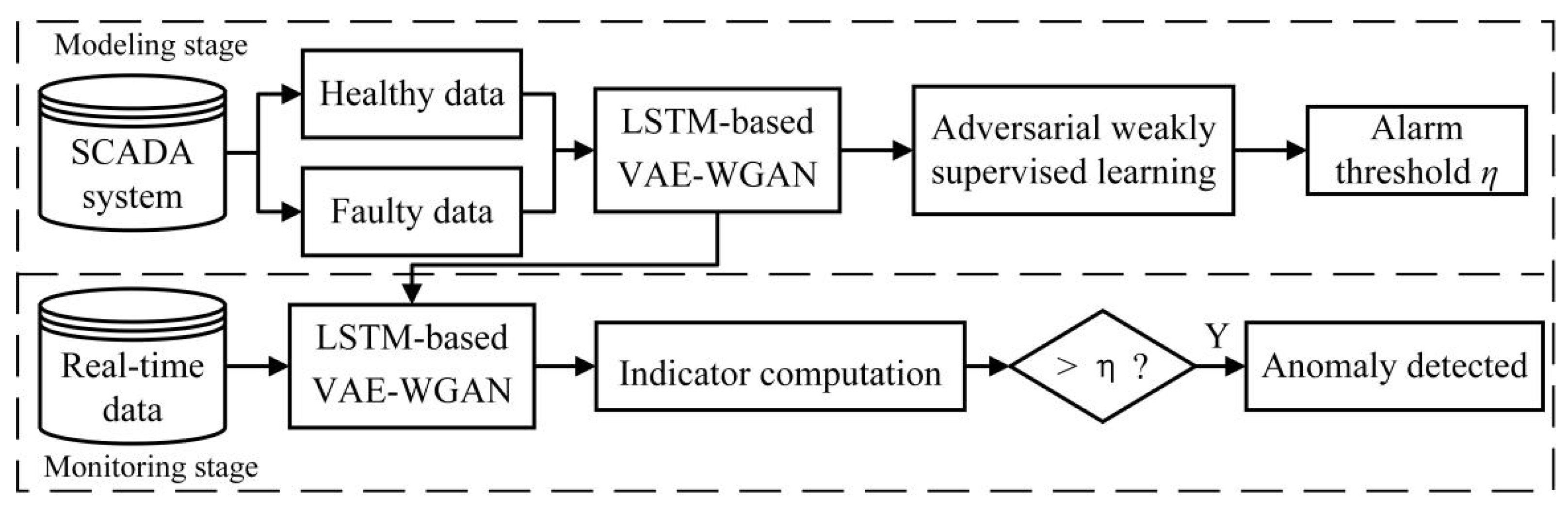
2.3. Anomaly Detection

The interdependence of SCADA variables remains stable under normal operating conditions but is inevitably disrupted in the presence of an anomaly. Once the LSTM-based VAE-WGAN model is effectively trained, the VAE demonstrates its capability to map inputs to a latent space and accurately reconstruct them back to their original form. The reconstruction error can thus be regarded as a suitable metric for anomaly detection, triggering an alarm when it surpasses a predefined threshold. Thus, the anomaly score is defined as shown below:

$$Anomaly score= ||x-\tilde{x}|{|}_2$$

(10)

The samples exhibiting high anomaly scores are classified as anomalies according to a predetermined threshold $\eta$. Additionally, KDE is utilized to fit the distribution of anomaly scores under normal conditions and to subsequently calculate the Probability Density Function (PDF) as:

$$\stackrel{\wedge }{f}(x)=\frac{1}{nh}{\displaystyle \sum _{k=1}^{n}K(\frac{x-x_k}{h})}$$

(11)

where $K(\cdot )$ represents the kernel function under the condition of ${\displaystyle {\int }_{-\infty }^{+\infty }K(x)dx=1}$, $x_k$ denotes the element contained, and $h$ denotes the window width to ensure that the estimated $\stackrel{\wedge }{f}(x)$ can best fit the distribution. In this study, the Gaussian kernel function was chosen for $K(\frac{x-x_k}{h})=\frac{1}{h\sqrt{2\pi }}{e}^{-\frac{{(x-x_k)}^2}{2h^2}}$.

The alarm threshold $\eta$ at a given confidence interval of $\alpha$ can be obtained below. Additionally, the mechanism is defined here that an alarm will only be issued when certain consecutive points exceed the threshold.

$$\alpha =P(x<\eta )={\displaystyle {\int }_0^{\eta }\stackrel{\wedge }{f}(x)dx}$$

(12)

3. Results

The following section provides specific examples from a wind farm situated in northeast China to validate the feasibility and advancement of the proposed model. The wind turbines are identical in type, featuring a rated power output of 2.6 MW, rotor diameter of 140 m, hub height of 100 m, cut-in speed of 2.5 m/s, rated wind speed of 8.5 m/s, cut-out speed of 20 m/s, and rated generator speed at 1750 rpm with a design life set for twenty years.

3.1. Generator Input Bearing Wear for Wind Turbine YD37

Pitting corrosion of the generator input bearing was found for wind turbine YD37 during a planned inspection on 25 October 2021, which must be replaced after a subsequent detailed inspection. The LSTM-based VAE-WGAN was established for the generator with the input features of wind speed, output power, nacelle temperature, generator input shaft temperature, generator output shaft temperature, generator winding U temperature, generator winding V temperature, generator winding W temperature, and generator speed. The training parameters for this case are listed in

Table 1. Training network parameters for case one.

Training Network	Value
VAE network	[8 6 4 6 8]
Discriminator network	[6 2 1]
Batch size	64
Epoch size	2000
Delay time for LSTM [14]	10
Learning rate $\alpha$	0.001
Clipping parameter $c$	0.002
Discriminator iterations $n_{dis}$	5
VAE hyperparameter $\beta$	0.008
Gradient penalty weight $\lambda$	4

.

3.1.1. Model Performance

Comparative experiments were performed on the same training dataset with five different global random seeds, and the reconstruction results are presented in

Table 2. Comparative results of model performance for case one (normalized).

Training Network	MAE					RMSE
Random Seed	1	2	3	4	5	1	2	3	4	5
VAE	0.02062	0.01999	0.02106	0.01989	0.01815	0.02760	0.02683	0.02794	0.02670	0.02448
VAE-GAN	0.02333	0.01997	0.02090	0.02300	0.02288	0.03058	0.02718	0.02772	0.03063	0.02963
VAE-WGAN	0.01725	0.01844	0.01976	0.02197	0.02017	0.02335	0.02442	0.02618	0.02939	0.02632
LSTM-based VAE	0.01475	0.01428	0.01490	0.01832	0.01220	0.02011	0.02022	0.01989	0.02513	0.01691
LSTM-based VAE-GAN	0.01006	0.01218	0.01172	0.01556	0.01384	0.01482	0.01671	0.01653	0.02092	0.01891
LSTM-based VAE-WGAN	0.00921	0.01287	0.01059	0.01062	0.01053	0.01389	0.01790	0.01543	0.01539	0.01525

. The proposed LSTM-based VAE-WGAN demonstrates superior model performance by effectively extracting spatiotemporal factors, as represented by its significantly lower mean absolute error (MAE) and root mean square error (RMSE) for reconstructing real inputs. Especially, by adopting the LSTM module in the reconstruction model, the performance can be significantly improved, as evidenced by lower reconstruction errors observed in LSTM-based VAE, LSTM-based VAE-GAN, and LSTM-based VAE-WGAN compared to VAE, VAE-GAN, and VAE-WGAN. Also, by using the Wasserstein distance and enforcing the Lipschitz constraint on the discriminator, the performance of VAE-WGAN can be improved compared to its GAN counterpart.

Moreover, the effects of network parameters on model performance have also been discussed, as illustrated in Figure 6. Typically, a more complex network architecture yields improved feature extraction capabilities but an increased risk of overfitting. In this case, the VAE and discriminator networks are set as [8 6 4 6 8] and [6 2 1], respectively. Moreover, the hyperparameter $\beta$ assigns a weight to balance the trade-off between reconstruction and discrimination in the VAE’s loss function, while the clipping parameter $c$ and gradient penalty weight $\lambda$ determine model constraints in WGAN. Therefore, optimal values can be obtained with a minimal MAE and RMSE, with 0.008 for the VAE hyperparameter $\beta$, 0.002 for the clipping parameter $c$, and 4 for the gradient penalty weight $\lambda$, as can be seen in Table 1.

3.1.2. Anomaly Detection

To detect anomalies in time, the two-stage adversarial semi-supervised training method proposed above is adopted. Due to the previous extended shutdown of this wind turbine for fire safety renovations, there was a limited amount of continuous normal data available (from 7 October to 14 October with a 1-min interval) for data preprocessing and model training, which were split into 70% for training and 30% for testing. Moreover, to initialize the discriminator parameters, a small amount of abnormal data (about 30% of the normal data) was generated by applying a large disturbance to the temperature parameters associated with the generator.

The histogram and estimated PDF of the reconstruction error for the testing sets are presented in Figure 7a, with the anomaly detection threshold determined as 0.0014. A total of 6375 data points before the shutdown are used for validation, and the monitoring reconstruction error and detection threshold are shown in Figure 7b. The alarm signal is triggered when fifteen consecutive points exceed the threshold which is at the 314th data point. After that, a large number of out-limits can be seen before the planned inspection, which serve as indicators of deviations in the internal relationships between variables and a decline in performance. Especially, the original monitoring generator input shaft and output shaft temperatures for validation are illustrated in Figure 7c. Under normal circumstances, the input shaft temperature should be slightly higher than the output shaft temperature. However, during the validation period leading up to the shutdown, there is a significant disparity between the input and output shaft temperatures, which further intensifies over time. The traditional fixed-threshold alarm or trend alarm methods face challenges in deep and long-term dependency relations between monitoring parameters and detecting these changes, thus validating the effectiveness of the proposed method. The presence of several prominent columnar lines in Figure 7b marked by green ellipses, which are most likely attributed to interference during the measurement process (green ellipses in Figure 7c), is worth highlighting.

3.1.3. Comparative Experiments

For comparison, the detection results for this case using the LSTM-based AE [27], LSTM-based VAE [28], LSTM-based VAE-GAN, LSTM-based VAE-WGAN (without supervised pre-training for discriminator), LSTM-based VAE-WGAN (with supervised pre-training for discriminator) are illustrated in Figure 8. Among the 6375 validation data points, the point before the alarm is labeled as normal, whereas the remainder is labeled as abnormal. Subsequently, the precision, recall, and $F_1$ score are introduced as evaluation indicators, as expressed in Equations (13)–(15), respectively [29].

$$Precision=\frac{TP}{TP+FP}$$

(13)

$$Recall=\frac{TP}{TP+FN}$$

(14)

$$F_1=2\times \frac{Precision\times Recall}{Precision+Recall}$$

(15)

TP is the number of cases that are correctly labeled as positive, FP is the number of cases that are incorrectly labeled as positive, and FN is the number of cases that are positive but are labeled as negative. In particular, precision reflects the false alarm rate, whereas recall represents the missing alarm rate. The $F_1$ score reflects the balance between precision and recall, where a high score implies a good trained model. The detailed comparative results of different anomaly detection methods can be seen in

Table 3. Comparative results of different anomaly detection methods for case one.

Model	Alarm Point	Precision	Recall	F1 Score
LSTM-based AE	343rd point	0.9886	0.5476	0.7048
LSTM-based VAE	322nd point	0.9967	0.5944	0.7447
LSTM-based VAE-GAN	320th point	0.9942	0.7118	0.8296
LSTM-based VAE-WGAN(without supervised pre-training)	325th point	0.9944	0.7018	0.8229
LSTM-based VAE-WGAN (with supervised pre-training)	314th point	0.9952	0.7238	0.8381

. It is clear that the proposed LSTM-VAE-WGAN that adopts the two-stage adversarial semi-supervised training approach manages to capture subtle changes in the relationship between parameters with the earliest alarm point (314th point) and the highest $F_1$ score (0.8381). Thus, through deep and long-term dependency analysis between the monitoring parameters, as well as the initialization of discriminator parameters with abnormal data, the feasibility and advancement of the proposed model have been confirmed.

3.2. Sensor Failure of Pitch Motor Temperature 2 for Wind Turbine YD28

Sensor failure of pitch motor temperature 2 was found for wind turbine YD28 during a planned inspection on 15 October 2021. The LSTM-based VAE-WGAN was established for the pitch system with the input features of wind speed, output power, nacelle temperature, pitch torque 1, pitch torque 2, pitch torque 3, pitch motor temperature 1, pitch motor temperature 2, pitch motor temperature 3, pitch angle 1, pitch angle 2 and pitch angle 3. The training parameters for this case are listed in

Table 4. Training network parameters for case two.

Training Network	Value
VAE network	[8 6 4 6 8]
Discriminator network	[8 2 1]
Batch size	64
Epoch size	2000
Delay time for LSTM [14]	10
Learning rate $\alpha$	0.001
Clipping parameter $c$	0.002
Discriminator iterations $n_{dis}$	5
VAE hyperparameter $\beta$	0.008
Gradient penalty weight $\lambda$	4

.

3.2.1. Model Performance

Comparative experiments were performed on the same training dataset with five different global random seeds, and the reconstruction results are presented in

Table 5. Comparative results of model performance for case two (normalized).

Training Network	MAE					RMSE
Random Seed	1	2	3	4	5	1	2	3	4	5
VAE	0.03907	0.03640	0.03749	0.03913	0.03539	0.06099	0.05785	0.05682	0.05965	0.05827
VAE-GAN	0.03358	0.03443	0.03438	0.03517	0.03389	0.05635	0.05533	0.05489	0.05627	0.05652
VAE-WGAN	0.03243	0.03434	0.03490	0.03725	0.03238	0.05586	0.05593	0.05635	0.05765	0.05600
LSTM-based VAE	0.02861	0.02913	0.03011	0.02992	0.02663	0.04648	0.04664	0.04761	0.04704	0.04453
LSTM-based VAE-GAN	0.02592	0.02600	0.02934	0.02755	0.02719	0.04209	0.04294	0.04619	0.04419	0.04500
LSTM-based VAE-WGAN	0.02566	0.02737	0.02846	0.02648	0.02565	0.04395	0.04480	0.04621	0.04330	0.04405

. Similar to case one, the proposed LSTM-based VAE-WGAN achieves superior model performance by effectively extracting spatiotemporal factors, as demonstrated by its significantly lower MAE and RMSE for reconstructing real inputs.

The effects of network parameters on model performance have also been presented, as illustrated in Figure 9. The optimal network parameters can be obtained with [8 6 4 6 8] for the VAE, [8 2 1] for the discriminator, 0.008 for the VAE hyperparameter $\beta$, 0.002 for the clipping parameter $c$, and 4 for the gradient penalty weight $\lambda$ as can be seen in Table 4.

3.2.2. Anomaly Detection

To detect anomalies, normal data available from 1 October to 7 October with a 1-min interval were collected for data preprocessing and model training, which were split into 70% for training and 30% for testing. Also, a small amount of abnormal data (about 30% of the normal data) was generated by applying a large disturbance to the temperature parameters associated with the pitch system to initialize the discriminator parameters.

The histogram and estimated PDF of the reconstruction error for the testing sets are presented in Figure 10a, with the anomaly detection threshold determined as 0.016. A total of 5229 data points before the shutdown are used for validation, and the monitoring reconstruction error and detection threshold are shown in Figure 10b. The alarm signal is triggered when five consecutive points exceed the threshold which is at the 4639th data point. After that, a large number of out-limits can be seen before the planned inspection. The original monitoring pitch motor temperature 1 and pitch motor temperature 2 validation are illustrated in Figure 10c. Under normal circumstances, these two temperatures should be close to each other. During the validation period, however, a sensor failure in pitch motor temperature 2 resulted in an erratic fluctuation of the measured temperature, leading up to the out-limits of monitoring reconstruction error.

3.2.3. Comparative Experiments

For comparison, the detection results for this case using the LSTM-based AE, LSTM-based VAE, LSTM-based VAE-GAN, LSTM-based VAE-WGAN (without supervised pre-training for discriminator), LSTM-based VAE-WGAN (with supervised pre-training for discriminator) are illustrated in Figure 11, together with the detailed comparative results shown in

Table 6. Comparative results of different anomaly detection methods for case two.

Model	Alarm Point	Precision	Recall	F1 Score
LSTM-based AE	4867th point	0.6582	0.5746	0.6136
LSTM-based VAE	5140th point	0.2386	0.7640	0.3636
LSTM-based VAE-GAN	4812th point	0.5670	0.4365	0.4933
LSTM-based VAE-WGAN (without supervised pre-training)	4933th point	0.3450	0.3007	0.3213
LSTM-based VAE-WGAN (with supervised pre-training)	4639th point	0.6938	0.6220	0.6559

. Similar to case one, the proposed LSTM-VAE-WGAN that adopts the two-stage adversarial semi-supervised training approach manages to capture subtle changes in the relationship between parameters with the earliest alarm point (4639th point) and the highest $F_1$ score (0.6559).

4. Conclusions

In this study, the LSTM-based VAE-WGAN was established to address the challenge of small and noisy wind turbine datasets. The VAE was utilized as the generator, with LSTM units replacing hidden layer neurons to effectively extract spatiotemporal factors. The similarity between the model-fit distribution and true distribution was quantified using Wasserstein distance, enabling complex high-dimensional data distributions to be learned. Comparative experiments were conducted on the same dataset with five different global random seeds that the proposed LSTM-based VAE-WGAN achieved superior model performance by effectively extracting spatiotemporal factors, as demonstrated by its significantly lower mean absolute error (MAE) and root mean square error (RMSE) for reconstructing real inputs. The effects of network parameters on model performance have also been discussed. A more complex network architecture yields improved feature extraction capabilities but an increased risk of overfitting, while the VAE hyperparameter $\beta$, clipping parameter $c$, and gradient penalty weight $\lambda$ affect the training process of VAE and WGAN. Two real anomaly detection cases of pitting corrosion of the generator input bearing and sensor failure of pitch motor temperature 2 were represented. The histogram and estimated PDF of the reconstruction error for the testing sets by KDE, the monitoring reconstruction error and the detection threshold have been illustrated. The proposed method manages to mine deep and long-term dependency relations between the monitoring parameters and identify small changes in the relationships. Moreover, extensive comparative experiments with other anomaly detection methods were also conducted. The proposed LSTM-VAE-WGAN with the two-stage adversarial semi-supervised training approach achieved the best performance with the earliest alarm point and highest $F_1$ score.

Despite the above relevant findings, false alarms can still be seen in the real-time monitoring stage, and further research is needed to improve the model. Moreover, more complex and complete cases are needed to verify the wide applicability of the developed methods.

References

1. Mcmorland, J.; Collu, M.; Mcmillan, D.; Carroll, J. Operation and maintenance for floating wind turbines: A review. Renew. Sustain. Energy Rev. 2022, 163, 112499. [Google Scholar] [CrossRef]
2. Global Wind Report 2023. Available online: https://gwec.net/globalwindreport2023/ (accessed on 1 May 2023).
3. Bakir, I.; Yildirim, M.; Ursavas, E. An integrated optimization framework for multi-component predictive analytics in wind farm operations & maintenance. Renew. Sustain. Energy Rev. 2021, 138, 110639. [Google Scholar]
4. Zhu, Y.; Zhu, C.; Tan, J.; Song, C.; Chen, D.; Zheng, J. Fault detection of offshore wind turbine gearboxes based on deep adaptive networks via considering Spatio-temporal fusion. Renew. Energy 2022, 200, 1023–1036. [Google Scholar] [CrossRef]
5. Dhiman, H.S.; Deb, D.; Muyeen, S.M.; Kamwa, I. Wind Turbine Gearbox Anomaly Detection based on Adaptive Threshold and Twin Support Vector Machines. IEEE Trans. Energy Convers. 2021, 36, 3462–3469. [Google Scholar] [CrossRef]
6. Benammar, S.; Tee, K.F. Failure Diagnosis of Rotating Machines for Steam Turbine in Cap-Djinet Thermal Power Plant. Eng. Fail. Anal. 2023, 149, 107284. [Google Scholar] [CrossRef]
7. Nick, H.; Aziminejad, A.; Hosseini, M.H.; Laknejadi, L. Damage identification in steel girder bridges using modal strain energy-based damage index method and artificial neural network. Eng. Fail. Anal. 2021, 119, 105010. [Google Scholar] [CrossRef]
8. Li, H.; Huang, J.; Ji, S. Bearing Fault Diagnosis with a Feature Fusion Method Based on an Ensemble Convolutional Neural Network and Deep Neural Network. Sensors 2019, 19, 2034. [Google Scholar] [CrossRef] [PubMed]
9. Zhou, D.; Yao, Q.; Wu, H.; Ma, S.; Zhang, H. Fault diagnosis of gas turbine based on partly interpretable convolutional neural networks. Energy 2020, 200, 117467. [Google Scholar] [CrossRef]
10. Kong, Z.; Tang, B.; Deng, L.; Liu, W.; Han, Y. Condition monitoring of wind turbines based on spatio-temporal fusion of SCADA data by convolutional neural networks and gated recurrent units. Renew. Energy 2020, 146, 760–768. [Google Scholar] [CrossRef]
11. Yang, Z.; Baraldi, P.; Zio, E. A method for fault detection in multi-component systems based on sparse autoencoder-based deep neural networks. Reliab. Eng. Syst. Saf. 2022, 220, 108278. [Google Scholar] [CrossRef]
12. Xiang, L.; Yang, X.; Hu, A.; Su, H.; Wang, P. Condition monitoring and anomaly detection of wind turbine based on cascaded and bidirectional deep learning networks. Appl. Energy 2022, 305, 117925. [Google Scholar] [CrossRef]
13. Chen, H.; Liu, H.; Chu, X.; Liu, Q.; Xue, D. Anomaly detection and critical SCADA parameters identification for wind turbines based on LSTM-AE neural network. Renew. Energy 2021, 172, 829–840. [Google Scholar] [CrossRef]
14. Zhang, C.; Hu, D.; Yang, T. Anomaly detection and diagnosis for wind turbines using long short-term memory-based stacked denoising autoencoders and XGBoost. Reliab. Eng. Syst. Saf. 2022, 222, 108445. [Google Scholar] [CrossRef]
15. Khan, P.W.; Yeun, C.Y.; Byun, Y.C. Fault detection of wind turbines using SCADA data and genetic algorithm-based ensemble learning. Eng. Fail. Anal. 2023, 148, 107209. [Google Scholar] [CrossRef]
16. Liu, X.; Teng, W.; Wu, S.; Wu, X.; Liu, Y.; Ma, Z. Sparse Dictionary Learning based Adversarial Variational Auto-encoders for Fault Identification of Wind Turbines. Measurement 2021, 183, 109810. [Google Scholar] [CrossRef]
17. Dao, P.B. Condition monitoring and fault diagnosis of wind turbines based on structural break detection in SCADA data. Renew. Energy 2021, 185, 641–654. [Google Scholar] [CrossRef]
18. Morrison, R.; Liu, X.; Lin, Z. Anomaly detection in wind turbine SCADA data for power curve cleaning. Renew. Energy 2022, 184, 473–486. [Google Scholar] [CrossRef]
19. Morshedizadeh, M.; Rodgers, M.; Doucette, A.; Schlanbusch, P. A case study of wind turbine rotor over-speed fault diagnosis using combination of SCADA data, vibration analyses and field inspection. Eng. Fail. Anal. 2023, 146, 107056. [Google Scholar] [CrossRef]
20. Shen, X.; Fu, X.; Zhou, C. A combined algorithm for cleaning abnormal data of wind turbine power curve based on change point grouping algorithm and quartile algorithm. IEEE Trans. Sustain. Energy 2019, 10, 46–54. [Google Scholar] [CrossRef]
21. Chen, J.; Li, J.; Chen, W.; Wang, Y.; Jiang, T. Anomaly detection for wind turbines based on the reconstruction of condition parameters using stacked denoising autoencoders. Renew. Energy 2020, 147, 1469–1480. [Google Scholar] [CrossRef]
22. Thill, M.; Konen, W.; Wang, H.; Bäck, T. Temporal convolutional autoencoder for unsupervised anomaly detection in time series. Appl. Soft Comput. 2021, 112, 107751. [Google Scholar] [CrossRef]
23. Yong, B.X.; Brintrup, A. Bayesian autoencoders with uncertainty quantification: Towards trustworthy anomaly detection. Expert Syst. Appl. 2022, 209, 118196. [Google Scholar] [CrossRef]
24. Jin, U.K.; Na, K.; Oh, J.S.; Kim, J.; Youn, B.D. A new auto-encoder-based dynamic threshold to reduce false alarm rate for anomaly detection of steam turbines. Expert Syst. Appl. 2022, 189, 116094. [Google Scholar]
25. Sun, C.; He, Z.; Lin, H.; Cai, L.; Cai, H.; Gao, M. Anomaly detection of power battery pack using gated recurrent units based variational autoencoder. Appl. Soft Comput. 2023, 132, 109903. [Google Scholar] [CrossRef]
26. Gulrajani, I.; Ahmed, F.; Arjovsky, M.; Dumoulin, V.; Courville, A.C. Improved Training of Wasserstein GANs. In Proceedings of the 31st International Conference on Neural Information Processing Systems (NIPS’17), Long Beach, CA, USA, 4–9 December 2017; Curran Associates Inc.: Red Hook, NY, USA, 2017; pp. 5769–5779. [Google Scholar]
27. Hu, D.; Zhang, C.; Yang, T.; Chen, G. Anomaly Detection of Power Plant Equipment Using Long Short-Term Memory Based Autoencoder Neural Network. Sensors 2020, 20, 6164. [Google Scholar] [CrossRef]
28. Lin, S.; Clark, R.; Birke, R.; Schonborn, S.; Trigoni, N.; Roberts, S. Anomaly Detection for Time Series Using VAE-LSTM Hybrid Model. In Proceedings of the ICASSP 2020—2020 IEEE International Conference on Acoustics, Speech and Signal Processing (ICASSP), Barcelona, Spain, 4–8 May 2020. [Google Scholar]
29. Hu, D.; Zhang, C.; Yang, T.; Chen, G. An Intelligent Anomaly Detection Method for Rotating Machinery Based on Vibration Vectors. IEEE Sens. J. 2022, 22, 14294–14305. [Google Scholar] [CrossRef]
Figure 1. Flowchart of proposed anomaly detection procedure.
Energies 16 07008 g001
Figure 2. Structure diagram of a VAE.
Energies 16 07008 g002
Figure 3. Structure diagram of a GAN.
Energies 16 07008 g003
Figure 4. Structure diagram of an LSTM.
Energies 16 07008 g004
Figure 5. Structure diagram of the LSTM-based VAE-WGAN.
Energies 16 07008 g005
Figure 6. Effects of network parameters for case one: (a) VAE network; (b) Discriminator network; (c) VAE hyperparameter β ; (d) Clipping parameter c ; (e) Gradient penalty weight λ .
Energies 16 07008 g006
Figure 7. Anomaly detection for case one: (a) Histogram and density estimation by KDE; (b) Monitoring reconstruction error; (c) Monitoring temperature.
Energies 16 07008 g007
Figure 8. Anomaly detection results for case one: (a) LSTM-based AE; (b) LSTM-based VAE; (c) LSTM-based VAE-GAN; (d) LSTM-based VAE-WGAN (without supervised pre-training for discriminator).
Energies 16 07008 g008
Figure 9. Effects of network parameters for case two: (a) VAE network; (b) Discriminator network; (c) VAE hyperparameter β ; (d) Clipping parameter c ; (e) Gradient penalty weight λ .
Energies 16 07008 g009
Figure 10. Anomaly detection for case two: (a) Histogram and density estimation by KDE; (b) Monitoring reconstruction error; (c) Monitoring temperature.
Energies 16 07008 g010
Figure 11. Anomaly detection results for case two: (a) LSTM-based AE; (b) LSTM-based VAE; (c) LSTM-based VAE-GAN; (d) LSTM-based VAE-WGAN (without supervised pre-training for discriminator).
Energies 16 07008 g011