Analysis of the Influencing Factors of the Leak Detection Method Based on the Disturbance-Reflected Signal

Abstract

Leak detection technology, based on the disturbance-reflected signal, can realize pipeline state inspection without relying on the transient characteristics of leakage. However, the lack of research on the factors affecting the detection effect of this method greatly restricts its popularization and application. Therefore, this paper realizes the valve opening and closing through dynamic mesh technology and further establishes a 2D pipeline disturbance and reflection signal detection model. The correctness of the computational fluid dynamics (CFD) model detection mechanism was verified by theoretical analysis and indoor pipe flow experiments. In this process, it was found that reflections from boundaries, such as the pipe end, could also be identified and did not interfere with leak-related signals. In addition, the positioning errors of the leakage hole and the pipe end were 4.447% and 0.121%, respectively, and accurate positioning with zero error was able to be achieved in the calculation results of the CFD model. Finally, the influence factors of the detection effect of this method were analyzed by inputting the determined disturbance signal. Both the disturbance signal characteristics and the leakage hole characteristics affected the reflected signal, and the former played a more prominent role. Surprisingly, the results showed that pipeline flow and pressure had very limited influence on this method.

1. Introduction

Pipeline transportation, the most efficient and environmentally friendly method at present, makes it possible for fluid to be transported continuously [1,2,3]. However, leakage is always one of the key problems that troubles the smooth operation of pipelines, which brings a great threat to the surrounding life safety, the environment, and property [4,5]. Therefore, research on leak detection technology of oil and gas pipelines is of great significance to ensure the safe operation of pipelines. Fortunately, there have been numerous reports of leak detection [6,7,8], and many detection technologies have been proposed after a long period of research, which can be broadly divided into two categories: one is software-based technology, and the other is hardware-based technology. The former mainly includes leakage detection technologies based on signal processing, such as volume/flow balance [9], real-time model [10], and the negative pressure wave method [11,12,13], etc. They depend primarily on the pipeline supervisory control and data acquisition (SCADA) system to provide data sources. The latter mainly includes the optical method [14,15], the acoustic method [16,17], the distributed optical fiber sensor [18,19], chemical composition analysis [20], and others. Many of these methods use signal processing to capture key information for leak detection.

The demand for safe and economical pipeline transportation promotes the development of pipeline leak detection technology. Hu et al. [17] and Liu et al. [21] compared the advantages and disadvantages of different detection technologies and found that acoustic detection technology is a comprehensive and balanced method. With the continuous optimization of detection equipment, the recognition accuracy is improving [1,22]. Meanwhile, the increase in transportation demand leads to the complex structure and large scale of the pipeline network, which will produce a large amount of pipeline data. Finding pipeline leaks in such large amounts of data is costly and time-consuming. Thus, some machine learning and intelligent algorithms are gradually coming into view. Li et al. [23] used acoustic emission sensors to obtain the acoustic signal of leakage as the feature source. Data features were dimensionally reduced using kernel principal component analysis, and the leakage was identified by the support vector machine. In addition, for leakage detection based on acoustic emission technology, Banjara et al. [24] developed a hyperplane using a support vector machine and an associated vector machine to establish a recognition algorithm. The algorithm, combined with binary classification, can realize the detection of leakage. Ning et al. [25] proposed a leak detection method based on SE-CNN. Spectrum enhancement (SE) technology was used for signal preprocessing to improve the signal-to-noise ratio, and a convolutional neural network (CNN) was selected to realize automatic leak feature recognition from preprocessed signals. Based on pressure/flow data under different leakage conditions generated by OLGA software, Zadkarami et al. [26] took the statistical characteristics and wavelet characteristics as the input of the multi-layer perceptron neural network to realize the identification and diagnosis of the pipeline leakage state.

However, pipeline leakage accidents more or less will cause losses. Therefore, some scholars began to analyze the pipeline failure process so that pipeline leakage can be predicted in advance, and accidents can be avoided. Given the phenomenon of pipeline failure caused by third-party damage, corrosion, and other factors, which are the main causes of pipeline accidents, prediction models based on accident tree [27], Bayesian theory [28,29], structural reliability analysis [30], and other methods were established to analyze the possibility of pipeline failure and realize early warning, which can provide sufficient time for the layout of emergency response measures [31]. These models tend to predict results in probabilistic terms, so failure models can often be used in conjunction with leak detection methods to achieve better results. Unfortunately, in most detection methods based on signal processing, the key to leakage detection and location is to capture the transient signal caused by the leakage. However, some slowly developing leaks, such as leak holes formed by the slow development of local pitting, cannot generate enough transient characteristics. Therefore, the disturbance was introduced into the pipeline, and the influence of the leakage hole on the disturbance signal was analyzed to obtain the relevant information about the leakage hole.

Brunone et al. [32,33,34,35,36,37] have extensive research experience in this area. They proposed a method of leakage detection for drainage pipes based on reflected signals, and wavelet transform was introduced for signal decomposition and recognition. The attenuation law of pressure signal was summarized by employing experimentation and simulation. They believed that pressure signal attenuation was exponentially related to the size, location, and pressure of the leakage hole. Then, based on these findings, they designed a portable pressure wavemaker (PPWM) device to generate transient disturbances to detect abnormal pipeline states. In addition, the system frequency response diagram was selected as the index of pipeline integrity by Lee et al. [38], and a method to determine the state of the leakage hole was established by analyzing the extraction method of frequency response, measurement position, noise interference, and other factors. Mpesha et al. [39] obtained the frequency response by using the transfer matrix method to conduct frequency domain analysis on the oscillating flow generated by opening and closing the valve periodically. Guo et al. [40] used the first transient pressure shock to detect the leakage with the help of numerical simulation and experimentation and established the relationship between leakage and reflection. Liao et al. [41] and Kim [42], respectively, introduced deep learning into the framework of transient frequency response to realize leak identification and estimate the leakage amount. It is worth mentioning that switching valve states quickly is one of the simplest ways to introduce a disturbance signal into the pipeline, which is usually selected to analyze reflected signals in pipeline leakage [43,44].

The leakage detection technology based on disturbance response can make up for the shortcomings of most detection methods based on signal processing, which rely on the transient response of the pipeline. At present, most efforts are focused on analyzing the reflected signal to locate the leak. This process mainly involves the attempt of different data processing algorithms, the application of different experimental systems, and the combination with deep learning methods. However, to the best of our knowledge, few studies have analyzed the influencing factors of the reflected signal, and most disturbance signals are generated by switching valve states, which is difficult to quantitatively analyze. The lack of research results limits the popularization and application of this method. Fortunately, the CFD method can accurately control the changes of different influencing factors. Therefore, a 2D simulation model based on dynamic mesh technology was established in this work. An indoor loop experiment was carried out to verify this model, and the accuracy of the leakage location was analyzed. The influence of pipeline operation parameters on transient response was obtained by analyzing the characteristics of reflected signals.

2. CFD Simulation

2.1. Geometric Model and Computational Grids

A two-dimensional simulation model was established, of which the total length and inner diameter were 12 m and 42 mm, respectively. As shown in Figure 1, two leakage holes, hole A and hole B, with sizes of 2 mm, were set on the pipeline, of which the distances to the inlet of the pipeline were 3 m and 8 m, respectively. Leakage hole A was the leak point to be detected, and as shown in Figure 2a, it consisted of nothing more than a short tube C, which was 10 mm long. Leakage hole B was a switchable valve used to provide a disturbance signal. As shown in Figure 2b, it was composed of short tube A and short tube B, and a valve was connected in the middle. The lengths of tube A, valve, and tube B were 5 mm, 3 mm, and 2 mm, respectively. The lower ends of the leakage holes A and B were connected to the pipe, and the upper ends were connected to the air. In addition, monitoring points were set at 1 m, 4 m, 7 m, and 10 m from the starting point of the pipeline, respectively. At the same time, the pressure at the outlet of the leakage hole was lower than the pipeline pressure but higher than the atmospheric pressure. It was difficult to determine this pressure boundary directly. Thus, a sufficiently large area of atmospheric air, which was 5 m high, 8 m wide, and could cover two leak holes horizontally, was provided to calculate the boundary pressure.

A 2D structured mesh was generated from the geometric model. Due to the large pressure gradient at the leakage point, the local grid was encrypted. To truly restore the flow state of the fluid at the leakage hole when the valve is opened or closed, dynamic mesh technology was used to simulate the valve transition. At first, valve A was closed, as shown in Figure 3a, and the fluid in the pipe flowed normally into a stable state. At 3 s, the valve body began to rotate counterclockwise around its centroid at an angular speed of 12 rad/s. As shown in Figure 3b, at 3.1 s, the valve was fully open. Figure 4 shows the distribution of the phase fraction. Red represents water, and blue represents air. It can be seen that the valve body was filled with air before the valve was opened, and the fluid in the tube entered the body after the valve was opened.

The mesh independence was verified by doubling the mesh density several times, as shown in

Table 1. Table of different mesh sizes.

Number	Pipeline	Valve	Tube	Air	Total
1	9854	6754	62	82	16,752
2	39,416	27,018	250	330	67,014
3	157,664	108,072	1000	1320	268,056
4	630,656	432,288	4000	5280	1,072,224

. Figure 5 was obtained by analyzing the flow velocity at monitoring points 1 and 3 when the valve was fully opened (3.1 s). The results showed that the first encryption greatly affected the calculation results, but the second and third encryptions had little effect. Considering the calculation accuracy and calculation cost, mesh #2 was selected for simulation calculation.

2.2. Mathematical Model

The numerical simulation was carried out based on Ansys Fluent. Compressibility must be considered if the transient response of a fluid in a pipeline is analyzed. To facilitate experimental verification, water was selected as the flow medium, and its elastic modulus was set as E = 2.2 GPa. The SST k-ω turbulence model was selected to close the Reynolds-averaged Navier–Stokes equations. The process of water spraying into the air at the leakage was a multiphase flow, but this arrangement was simply to obtain an accurate pressure boundary. Thus, the mixture model with a lower computational cost was chosen. The continuity and momentum governing equations can be written as follows:

$$\frac{\partial }{\partial t}\left({\rho }_m\right)+\nabla \cdot \left({\rho }_m{\overrightarrow{v}}_m\right)=0$$

(1)

$$\frac{\partial }{\partial t}\left({\rho }_m{\overrightarrow{v}}_m\right)+\nabla \cdot \left({\rho }_m{\overrightarrow{v}}_m{\overrightarrow{v}}_m\right)=-\nabla p+{\rho }_m\overrightarrow{g}$$

(2)

$\overrightarrow{v_m}$ can be determined as:

$${\overrightarrow{v}}_m=\frac{{\displaystyle \sum _{k=1}^n{\alpha }_k}{\rho }_k{\overrightarrow{v}}_k}{{\rho }_m}$$

(3)

${\rho }_m$ can be determined as:

$${\rho }_m={\displaystyle \sum _{k=1}^n{\alpha }_k}{\rho }_k$$

(4)

where α is the phase volume fraction, and k and m represent the different phase and mixing phase, respectively.

2.3. Boundary Condition and Solution Strategy

In this work, the computed reference frame did not move, and the valve body rotated around its centroid. The valve could be opened and closed by a user-defined function (UDF). The DEFINE_CG_MOTION function was used to define a valve rotation angular speed of 12 rad/s, in which case, the valve could be fully opened within 0.1 s. The correctness of the method was proved by comparing it with experimental data. To ensure that the fluid flow could be realized when the valve was opened and the fluid flow could be completely cut off when the valve was closed, the interfaces between the short tubes and the valve body were set as the matching format, and there was no contact between the short tubes and valve body when the valve was closed. The inlet speed of the pipeline was set as 2 m/s, and the outlet pressure was 200 KPa. The boundary of the air area was set as pressure outlet P = 0 Pa, and the other boundaries were set as no-slip walls.

Furthermore, to analyze the influence of flow parameters inside the pipeline on this method, as shown in

Table 2. Parameter settings.

		Velocity/(m/s)	Pressure/kPa
Disturbance signal	1	$V_1=\left\{\begin{array}{ll}2& ,t<2\\ 2-0.4\times \sin \left(16t-0.191\pi \right)& ,2\le t\le 2.1\\ 1.6& ,t>2.1\end{array}\right.$	200
	2	$V_2=\left\{\begin{array}{ll}2& ,t<2\\ 2+0.4\times \sin \left(16t-0.191\pi \right)& ,2\le t\le 2.1\\ 2.4& ,t>2.1\end{array}\right.$	200
	3	$V_3=\left\{\begin{array}{ll}2& ,t<2\\ 2-0.4\times \sin \left(30t-0.9\pi \right)& ,2\le t\le 2.1\\ 2& ,t>2.1\end{array}\right.$	200
Flow rate	1	$V_4=\left\{\begin{array}{ll}1& ,t<2\\ 1-0.4\times \sin \left(16t-0.191\pi \right)& ,2\le t\le 2.1\\ 1& ,t>2.1\end{array}\right.$	200
	2	$V_5=\left\{\begin{array}{ll}3& ,t<2\\ 3-0.4\times \sin \left(16t-0.191\pi \right)& ,2\le t\le 2.1\\ 3& ,t>2.1\end{array}\right.$	200
Pressure	1	$V_6=\left\{\begin{array}{ll}2& ,t<2\\ 2-0.4\times \sin \left(16t-0.191\pi \right)& ,2\le t\le 2.6\\ 2& ,t>2.6\end{array}\right.$	100
	2	$V_7=\left\{\begin{array}{ll}2& ,t<2\\ 2-0.4\times \sin \left(16t-0.191\pi \right)& ,2\le t\le 2.6\\ 2& ,t>2.6\end{array}\right.$	200
	3	$V_8=\left\{\begin{array}{ll}2& ,t<2\\ 2-0.4\times \sin \left(16t-0.191\pi \right)& ,2\le t\le 2.6\\ 2& ,t>2.6\end{array}\right.$	300

, the boundaries were modified to introduce a clear disturbance function, which was generated by adding a sinusoidal wave, based on 2 m/s. Similarly, the influence of the size of the leakage hole was analyzed. The disturbance signal V₁ was set, and the outlet pressure was 200 kPa. The sizes of leakage holes were set as 1 mm, 2 mm, and 3 mm, respectively.

The PISO algorithm was selected to solve the pressure–velocity coupled equations. The momentum and turbulence equations were discretized by the second-order upwind scheme. The convergence criterion was set, as residuals of all the governing equations were less than 10⁻⁵. To obtain sufficient sampling frequency, the time step was set as 5 × 10⁻⁴.

3. Pressure Disturbance Experiment and Model Validation

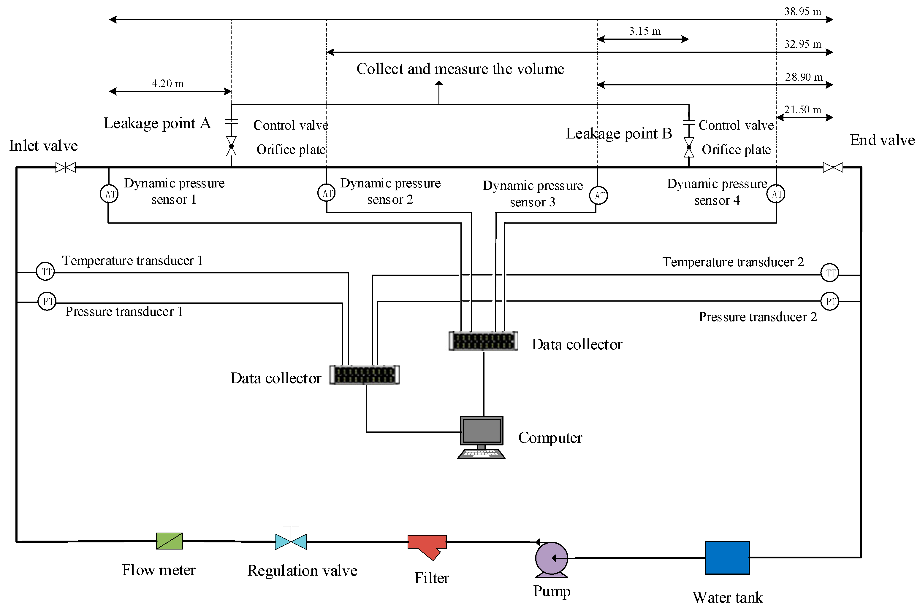
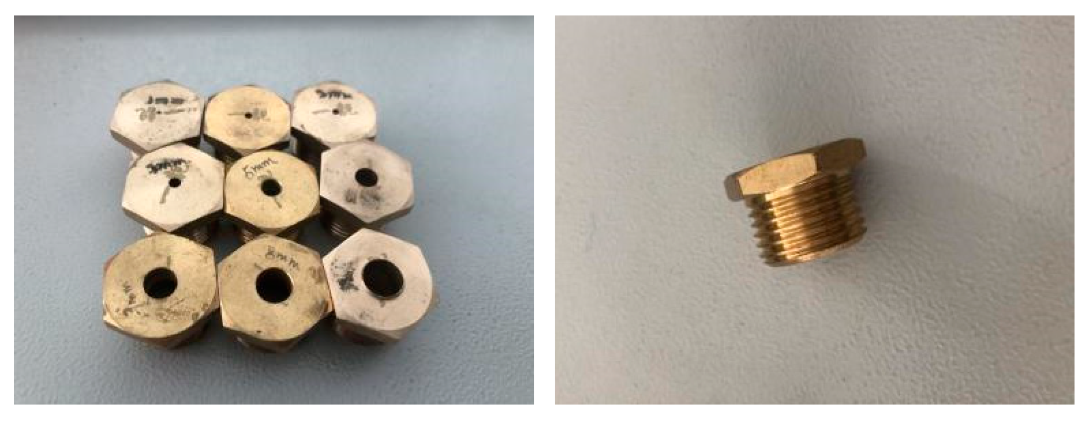
3.1. Pressure Disturbance Experiment

As shown in Figure 6, the experimental equipment consisted of two parts: the indoor pipe flow system and the data acquisition system. Figure 7 shows the indoor pipe flow system. The inner diameter, wall thickness, and length of the pipeline were 42 mm, 3 mm, and 110 m, respectively. Similar to the physical model of simulation calculation, there were two leakage points, A and B, on the pipeline. In addition, four pressure detection devices (dynamic pressure sensors 1, 2, 3, and 4) were installed at distances of 38.95 m, 32.95 m, 28.90 m, and 21.50 m, respectively, to the end valve. Leakage point A, distributed between sensors 1 and 2, was 4.20 m away from sensor 1. Leakage point B, distributed between sensors 3 and 4, was 3.15 m away from sensor 3. The leakage point consisted of a ball valve and a leakage orifice plate shown in Figure 8. The simulation of leakage conditions was achieved by rapidly opening and closing the valve connected to the leak hole. The pipeline was powered by a centrifugal pump (EVMSG20 15F5HQ1BEGE/18. 5, EBARA MACHINERY CO., LTD, Beijing, China). The outlet and inlet of the pipeline were connected to the water tank to realize the inner circulation of water.

The data acquisition system consisted of a central control system and a dynamic pressure signal acquisition system. Gauges, such as pressure sensors (meaconMIK-P300) and flow meters (meaconMIK-LWGY) installed along the pipeline, were linked to the central control system. The data detected by gauges were transmitted to the monitoring host through the pre-amplification device, I/V board, stabilized power supply, analog filter, and data acquisition card, respectively. Parameters such as pressure, temperature, and mass flow along the pipeline were detected by the monitoring host to determine the experimental conditions. The dynamic pressure signal acquisition system was mainly used to monitor and record the transient signal data of pipelines. The measuring range of the dynamic pressure sensor (PCB, 106B) was 0~57.3 kPa. The sensitivity was 43.5 mV/kPa, and the low-frequency response was 0.5 Hz.

The flow parameters were adjusted to the set conditions by starting the power system and regulating the pipeline valves. After the pipeline operation entered a stable state, the experiment was carried out, and the valve at the leakage point was rapidly regulated to introduce disturbance signals:

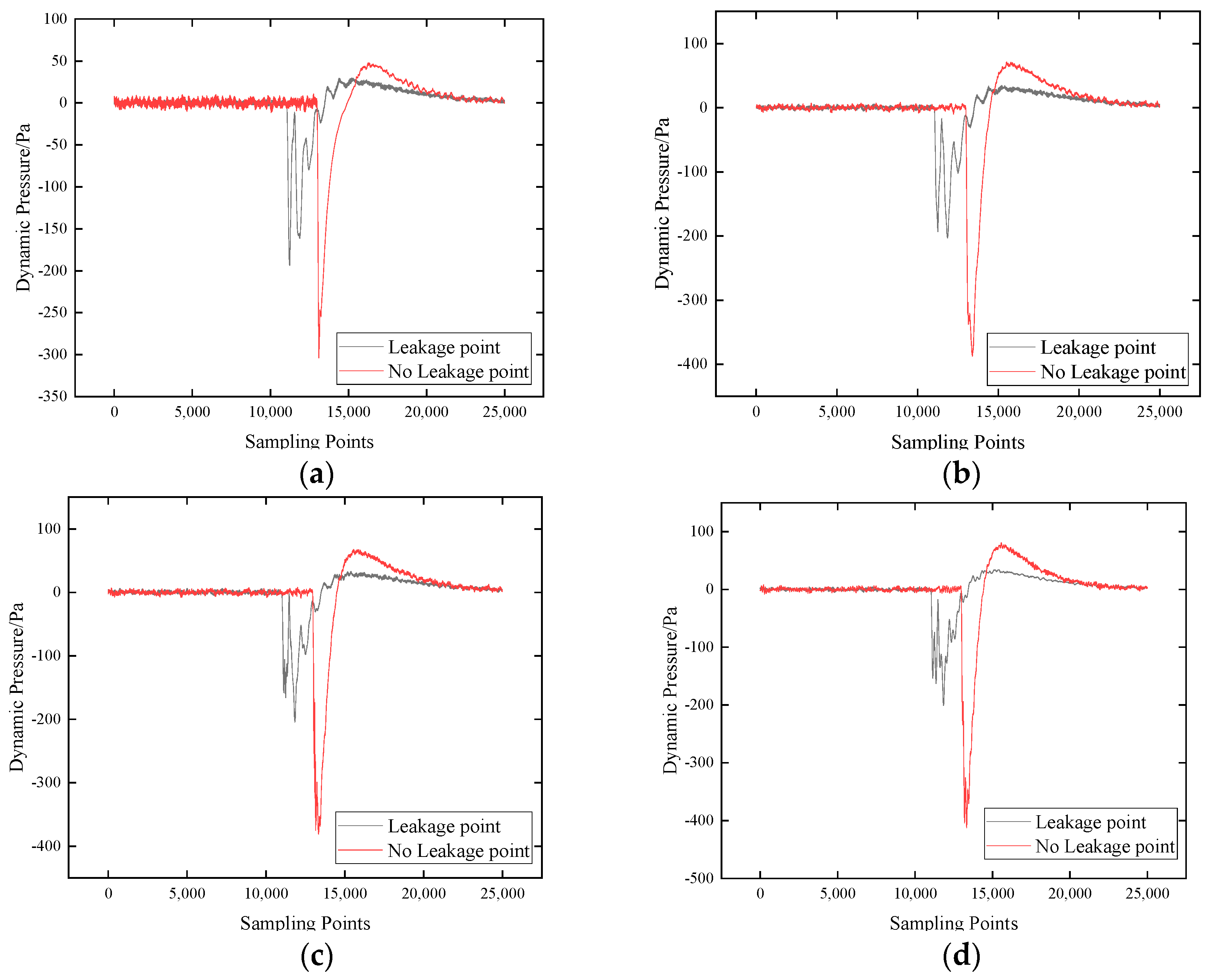
• The leakage orifice plates were separately installed at leakage points A and B. Leakage point A was opened, and then leakage point B was switched quickly until the pipeline entered a stable condition. The leakage point was closed after the acquisition of the dynamic pressure signal. This procedure was repeated many times through replacing the pressure levels and the sizes of the leakage orifice plates to complete the detection experiment with leakage points.
• The procedure was the same as the first step, except that leak point A was closed. This procedure was repeated many times through replacing the pressure levels and the sizes of the leakage orifice plates to complete the detection experiment without leakage points.

3.2. Model Validation

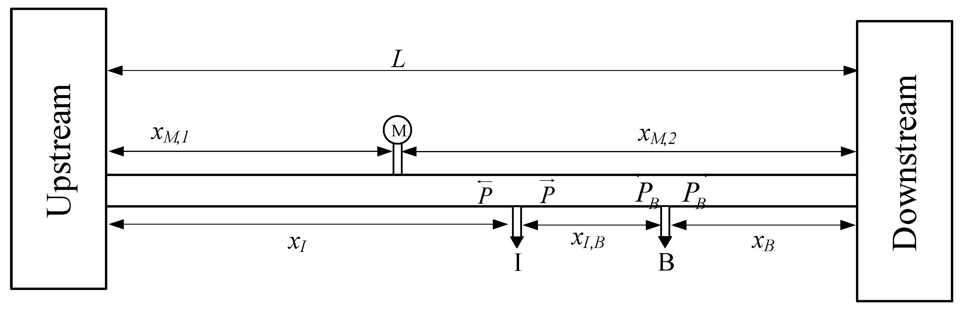
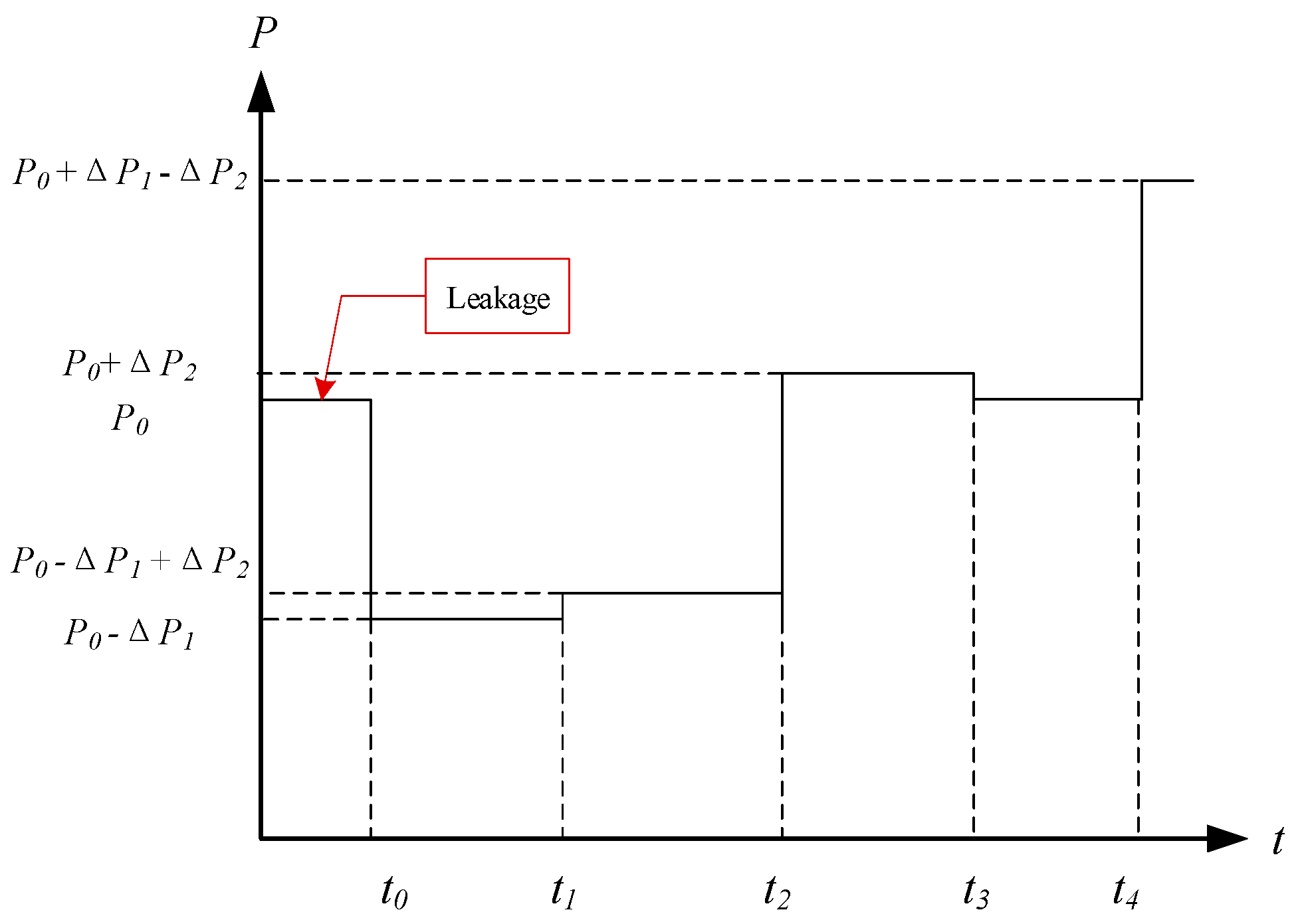
3.2.1. Reflection Analysis of Disturbing Signals under Ideal Conditions

In the piping system shown in Figure 9, the total length is L, and M is the pressure sensor. The propagation velocity of the pressure signal is a, and B is the unknown leakage point to be detected. When the transient leakage signal is generated at I, without considering the energy loss, the pressure fluctuations received by sensor M should show the pattern shown in Figure 10.

When the disturbance signal $\overrightarrow{P}$ is transmitted to the unknown leakage point B, the decompression wave leads to the pressure difference inside and outside of the pipeline decreasing. The fluid loss at the leakage hole is reduced, generating a pressure boost wave signal P_B. In the same way, P_B transfers to both sides of the upper and lower pipeline from the leakage point, resulting in the downstream signal ${\overrightarrow{P}}_B$ being superimposed on the original signal $\overrightarrow{P}$, which induces the value of signal $\overrightarrow{P}$ to decrease. This stacked signal propagates to the downstream boundary and reflects to form a boost wave. When it passes through the leakage hole, it will also generate a new reflection, but the effect of this signal is slight, which can be ignored. The signal captured by sensors at t₄ is characterized as a pressure rise (ΔP₁ − ΔP₂). The new signal transmitted upstream propagates to M at t₁, which is captured by the sensor, showing the pressure rise ΔP₂. This signal is reflected at the upstream boundary, forming the decomposition wave. Then, it is detected by sensor M, showing a pressure drop at t₃.

3.2.2. Reflection Analysis of Disturbing Signals under Experimental Conditions

In this work, dynamic pressure refers to the pressure difference before and after a unit sampling interval. It can be calculated as P_d = (P_n+1 − P_n)/Δt, where P_d is the dynamic pressure, P is the sampling pressure, n is the number of samples, and Δt is the sampling interval. Through de-noising processing based on wavelet transform, the comparison diagram of dynamic pressure signals obtained by four sensors under two conditions is illustrated in Figure 11. The black curve represents leakage point A (the leakage point to be detected), with a 1 mm orifice plate continuously leaked, and the leakage point B (the disturbance signal), with a 3 mm orifice plate that is switched on quickly. The red curve represents another condition where the leakage point B (the disturbance signal), with a 3 mm orifice plate, is only switched on quickly. Compared to the condition without leakage points to be detected, the amplitude of the collected dynamic pressure signals decreased significantly, and multiple peak characteristics appeared when there was a leakage point, which was due to the losses and the reflection of the energy when the pressure waves passed through leakage point A.

Under the condition that the pressure is 450 kPa, the leakage point A (to be detected), with a 1 mm orifice plate, kept leaking, and the leakage point B (the disturbance signal), with a 3 mm orifice plate, was opened rapidly. The dynamic pressure signals processed by the de-noising processing, based on wavelet transform, are shown in Figure 12. Because sensor 1 was located upstream of leak hole A, the reflected signal generated by the leak would overlap with the original signal and could not be identified. To reduce the relative error, sensor 4, which was furthest from the leakage point, was selected for analysis. The pressure wave propagation velocity was determined to be 1041.504 m/s, according to sensors 1 and 4, based on Equation (5) [45].

As shown in Figure 12, peak II was the disturbance signal generated by leakage point B. It was found by calculation that the distance between peak II and peak III was 16.6214 m. However, according to the design of the loop system, the distance (converted by the time difference) between the disturbance signal and the reflected signal detected by sensor 4 should be 18 m. Combined with the results of the theoretical analysis, it can be inferred that peak Ⅲ was the reflected wave of leakage point A, and the error was 7.6%. Similarly, peak IV was the end-reflected wave of peak II, and the error was 0.121%. Leakage led to gas–liquid two-phase flow in the pipe, which made the pressure wave propagation velocity change within a small range instead of a constant in the calculated pipe section [46]. Therefore, the calculation of the propagation distance lost some accuracy. The specific calculation is listed in

Table 3. Calculation of the reflected wave.

	Reflected Wave	Time/s	Distance/m	Actual Distance/m	Error/%
II-III	Leak point reflection	0.0158	16.6214	18	7.659
II-IV	End reflection	0.4485	47.307	47.25	0.121

. Then, according to Equation (5), the distance between the leakage hole and sensor 4 was calculated to be 12.661 m, while the actual distance was 13.25 m. The positioning error was 4.447%.

$$v_p=\frac{x_{M2}-x_{M1}}{t_{M2}-t_{M1}}$$

(5)

where v_p is the propagation velocity of the pressure wave, m/s; x_M1 and x_M2 are the locations of two detection points on the same side of the disturbance signal, m; and t_M1 and t_M2 represent the times when two sensors respectively received the disturbance signal, s.

3.2.3. Reflection Analysis of Disturbing Signals under Simulation Conditions

The static pressure–time data of each monitoring point were recorded and converted to dynamic pressure–time data to correspond to the experimental data. Figure 13 shows the dynamic pressure at monitoring point No. 3, with the valve fully open within 0.1 s. A solid black line indicates that there is no leak hole in the pipe, while the dotted red line indicates another situation. The change rule of the reflected signal calculated by the 2D model was the same as the theoretical analysis under ideal conditions and experimental data. In other words, the CFD model established in this work correctly described the generation and propagation laws of reflected signals. By comparing the variation trends of the two lines, it can be found that the presence of a leakage hole made the signal amplitude smaller and made the peak characteristics increase significantly. In addition, the pressure wave propagation velocity was calculated to be 1428.5714 m/s by the same processing method. The distance (by time difference conversion) between peak II and peak III was 1 m, which is exactly equal to the distance between leak hole A and monitoring point 3. The exact location of the leakage hole was realized because the propagation velocity of the pressure wave was accurately calculated.

4. Results and Discussion

The disturbance signal V₁ was analyzed as a representative, and the average flow velocity of the cross-section at leakage point A was monitored, as shown in Figure 14. Under the influence of the disturbance signal, the velocity at the cross-section decreased rapidly. Furthermore, the fluctuation of the transient velocity at the cross-section was far greater than the amplitude of the disturbance signal, and the velocity of the cross-section subsequently slowly returned to a stable state. This kind of phenomenon can be called the damping effect, which is caused by the continuity and inertia of the medium.

For the analysis of the disturbance signal, three representative signal types were set up, which represented the boost signal V₁, the decompression signal V₂, and the impulse pressure signal V₃, respectively. The pressure response of monitoring point 3 is shown in Figure 15a. When the opposite disturbance signal was introduced to the stable pipeline, the adverse pressure response was presented. The reflected signal caused by V₃ was significantly larger than the reflected signals caused by V₁ and V₂ because of the larger frequency of signal V₃. When comparing the values of I₁, I₂, and I₃, it was found that it was the temporal characteristics (frequency of disturbance signal) of the disturbing signal rather than the spatial characteristics (disturbance signal is a boost or decompress) that affected the amplitude of the reflected signal. The flow ejected from the leak hole would carry away some of the energy of the disturbance signal, which would be partly lost and partly converted into reflected waves to be transmitted to both ends of the leak hole. Keeping the size of the leakage hole constant, the high frequency of the disturbance signal would accelerate the change of pressure due to the hysteresis effect, leading to the leakage rate increase [47]. Therefore, the intensity of the reflected signal is positively correlated with the frequency of the disturbance signal.

As shown in Figure 15b, the amplitude of the disturbance signal increased with the increase of the leakage hole, while the amplitude of the reflection signal decreased with the increase of the leakage hole. This is because more energy will be lost through large leakage holes, resulting in the signals captured at the monitoring point being slightly weak. Although with the increase in the size of the leakage hole, the change rate of internal and external pressure differences decreased slightly, the leakage rate still showed an overall rising trend due to the increase in the size of the leak hole playing a dominant role, leading to the amplitude of the reflected signals being enhanced. In addition, the two cases of V₁ and V₃, as well as the leakage holes of 2 mm and 3 mm, were compared. Increasing the frequency by 1.875 times resulted in a 4-fold change in the amplitude of the reflected signal, while increasing the size of the leakage hole by 1.5 times resulted in only a 1.25-fold change in the amplitude of the reflected signal. It can be seen that the detection effect is more dependent on the characteristics of the disturbance signal rather than the characteristics of the leak hole. This is also unique to this approach.

Figure 15c,d shows the reflected signals under different flows and pressures, respectively. It can be seen that in each case, the reflected signals coincided almost exactly. Consequently, different flow and operation pressure hardly affected the detection effect. This is because the key factor affecting the disturbance response depends on the variation of the leakage flow rate. When the pipeline with leakage enters a stable flow state under different flow rates or pressure, the introduction of the same disturbance signal will cause the same pressure change at the leakage hole, and the change in leakage rate will be the same, which will generate the same reflection. In addition, the end reflection of the pipe was detected and located in the experiment and did not interfere with the leak hole information. It can be speculated that the elbow, reducer pipe, and other solid boundaries of the pipe will also produce reflections, which will also not interfere with leakage. However, due to the limitation of the experimental system, this part of the research has not been carried out. However, the design parameters of an in-service pipeline are all known. When the disturbance signal is introduced into the pipeline, the source of the reflected signal can be calculated according to these basic data. Furthermore, since the reflected signal is mainly affected by the characteristics of the disturbing signal, the same disturbance signal can be used to detect the pipeline. The reflected signal under normal conditions is recorded as the background value. A new reflected signal is obtained during pipeline status detection. Two signals are compared to find abnormal data, which can realize the exploration of leakage, during which, features such as elbows and variable diameters need not be considered.

5. Conclusions

In this paper, a 2D valve opening and closing leakage model was established, and the correctness of the model detection mechanism was verified by an indoor annular flow experiment and theoretical analysis. Sensitivity analyses of disturbance signal characteristics, leakage hole characteristics, and other factors were carried out. The main conclusions are as follows:

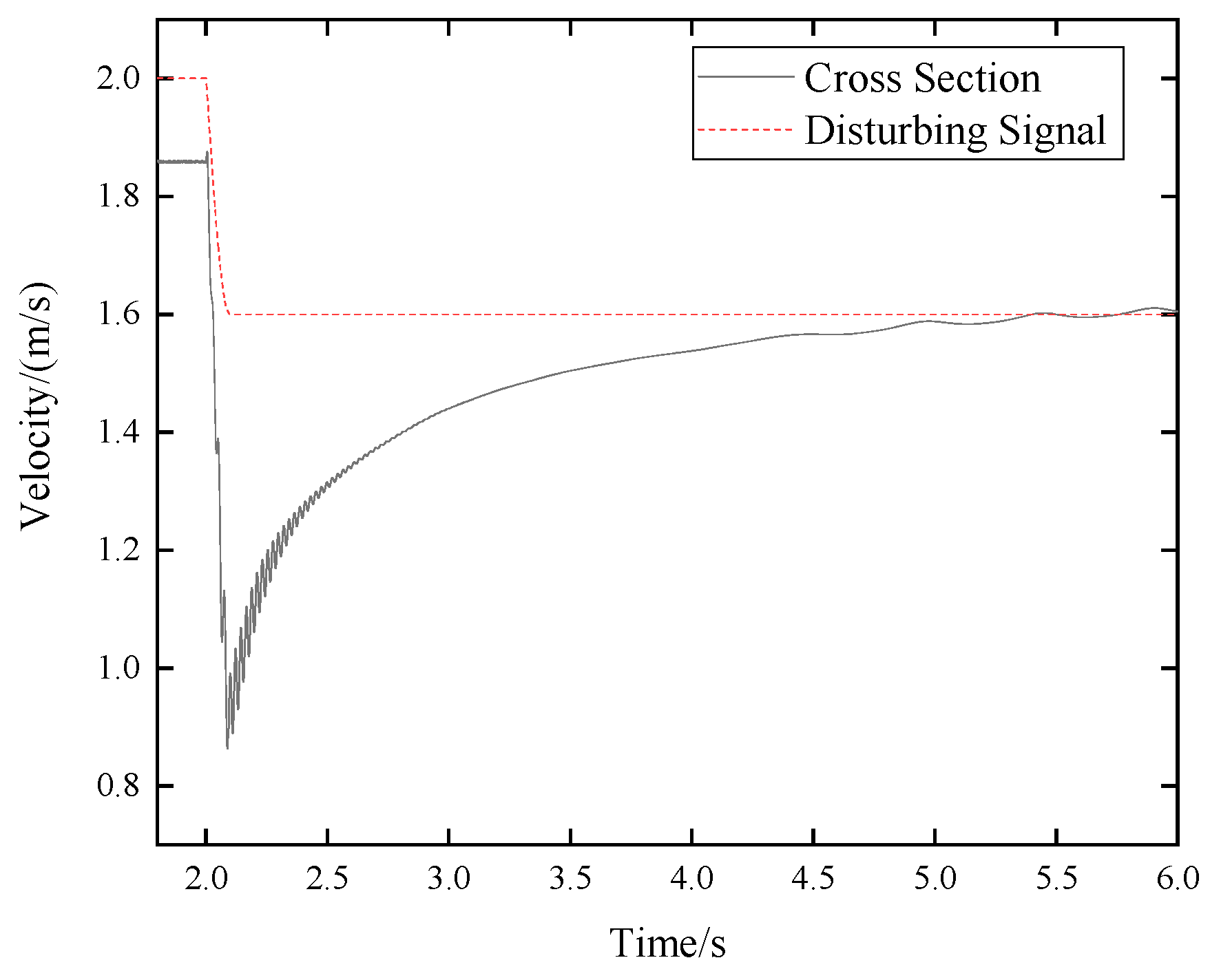
• The dynamic mesh technology can accurately control the valve opening and closing and realize the introduction of a disturbance signal. The 2D model can accurately locate the leakage position through the reflected signal.
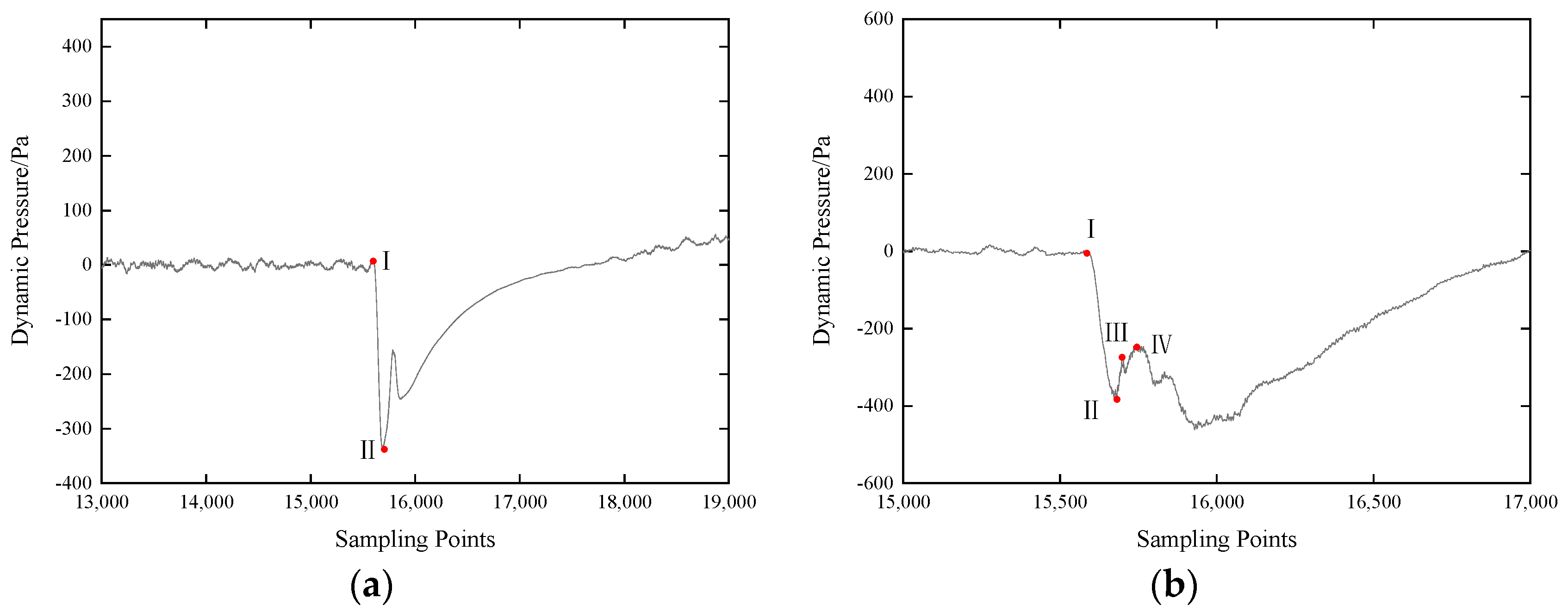
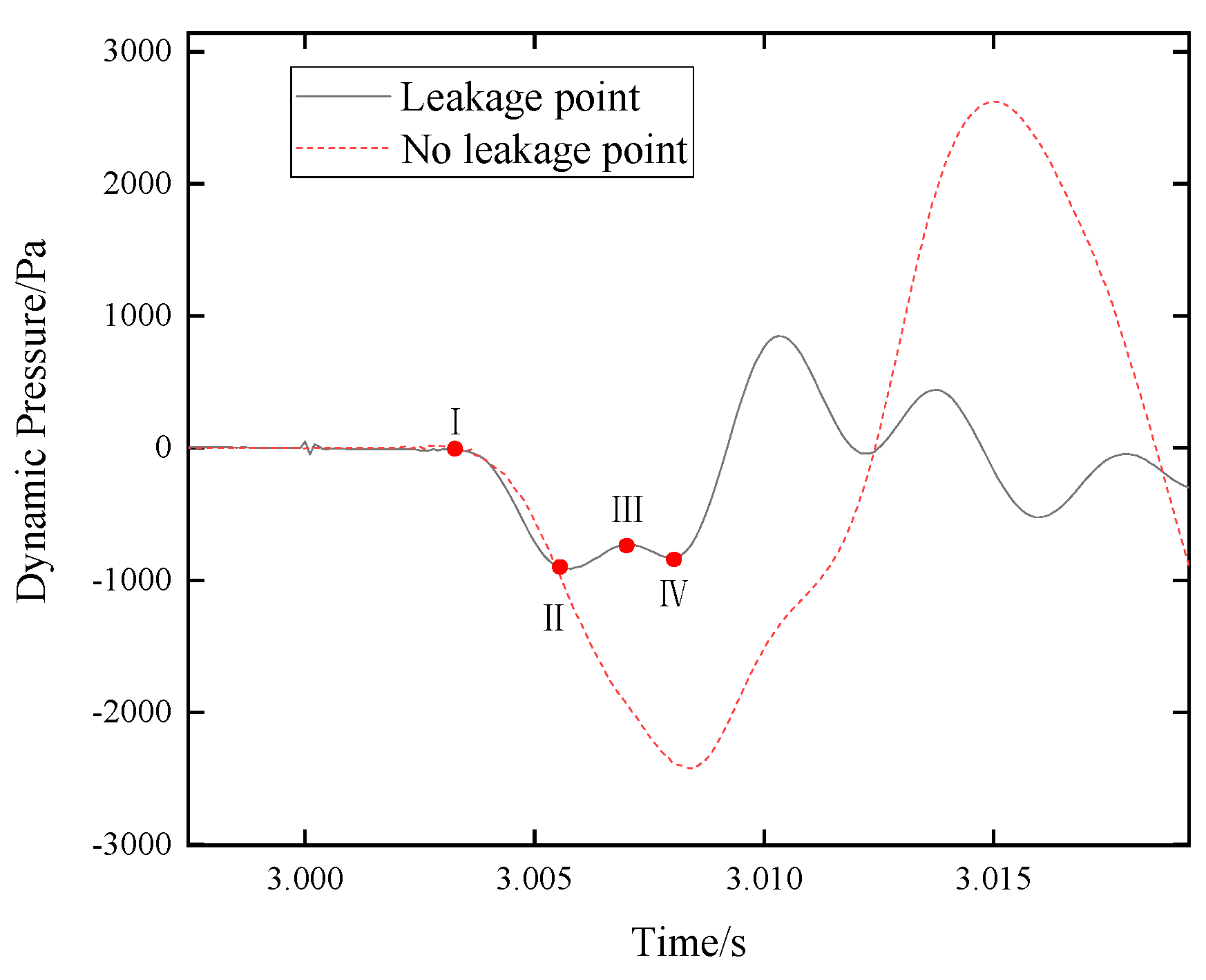
• Disturbance signal is introduced by quickly switching the valve in the experiment, and the location of the leakage hole is achieved by analyzing the reflection signal characteristics. The relative error between the actual distance (13.25 m) and the calculated distance (12.661 m) of the leakage hole positioning is 4.447%. A reflected signal is also generated at the end boundary of the pipe, and the relative error is only 0.121% when the position of the reflected signal source is calculated using this signal.
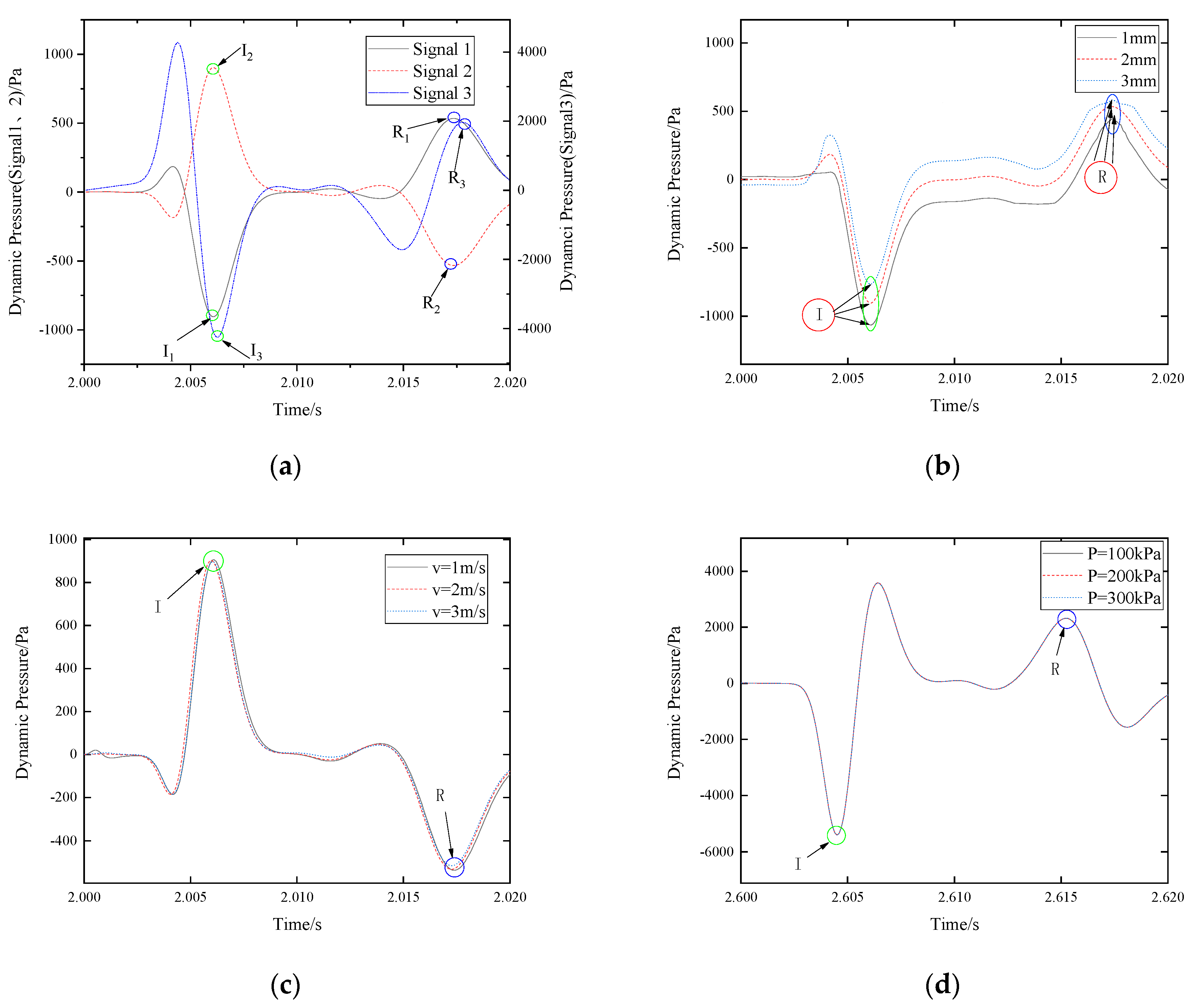
• The reflected signal is opposite to the disturbing signal. The amplitude of the reflected signal is positively correlated with the frequency of the disturbing signal, and the size of the leakage hole and the effect of the former are more prominent. However, the flow rate and the pressure of the pipeline have very limited influence on the reflected signal.

This work investigated leak detection techniques based on the disturbance-reflected signal, and the positioning accuracy was tested by an indoor circulation experiment. The influencing factors of the reflected signal were analyzed, and the sensitivity of each factor was ranked, which was helpful for the popularization and application of this technology and important for improving pipeline integrity management.

References

1. Zaman, D.; Tiwari, M.K.; Gupta, A.K.; Sen, D. A Review of Leakage Detection Strategies for Pressurised Pipeline in Steady-State. Eng. Fail. Anal. 2019, 109, 104264. [Google Scholar] [CrossRef]
2. Hankun, W.; Yunfei, X.; Bowen, S.; Chaoliang, Z.; Zhihua, W. Optimization and intelligent control for operation parameters of multiphase mixture transportation pipeline in oilfield: A case study. J. Pipeline Sci. Eng. 2021, 1, 367–378. [Google Scholar] [CrossRef]
3. Yi, W.; Junfei, L.; Baoqiang, J.I.; Jian, J. Influence of flow pattern on leakage acoustic signal of multiphase pipeline. Oil Gas Storage Transp. 2021, 40, 1138–1143. [Google Scholar] [CrossRef]
4. Chou, H.; Yeh, C.; Shu, C. Fire accident investigation of an explosion caused by static electricity in a propylene plant. Process. Saf. Environ. Prot. 2015, 97, 116–121. [Google Scholar] [CrossRef]
5. Bo, L.; Lan, H.Q.; Nan, L. Diffusion simulation and safety assessment of oil leaked in the ground. J. Pet. Ence Eng. 2018, 167, 498–505. [Google Scholar] [CrossRef]
6. Fu, H.; Yang, L.; Liang, H.; Wang, S.; Ling, K. Diagnosis of the single leakage in the fluid pipeline through experimental study and CFD simulation. J. Pet. Sci. Eng. 2020, 193, 107437. [Google Scholar] [CrossRef]
7. Fu, H.; Wang, S.; Ling, K. Detection of two-point leakages in a pipeline based on lab investigation and numerical simulation. J. Pet. Sci. Eng. 2021, 204, 108747. [Google Scholar] [CrossRef]
8. Molina-Espinosa, L.; Cazarez-Candia, O.; Verde-Rodarte, C. Modeling of incompressible flow in short pipes with leaks. J. Pet. Sci. Eng. 2013, 109, 38–44. [Google Scholar] [CrossRef]
9. Martins, J.C.; Seleghim, P. Assessment of the Performance of Acoustic and Mass Balance Methods for Leak Detection in Pipelines for Transporting Liquids. J. Fluids Eng. 2010, 132, 011401. [Google Scholar] [CrossRef]
10. Carvajal-Rubio, J.E.; Begovich, O.; Sanchez-Torres, J.D. Real-time leak detection and isolation in plastic pipelines with equivalent control based observers. In Proceedings of the 2015 12th International Conference on Electrical Engineering, Computing Science and Automatic Control (CCE), Mexico City, Mexico, 28–30 October 2015. [Google Scholar]
11. Sun, Y.W.; Zeng, B.Y.; Dai, Y.T.; Liang, X.J.; Zhang, L.J.; Ahmad, R.; Su, X.T. A novel hybrid technique for leak detection and location in straight pipelines—ScienceDirect. J. Loss Prev. Process. Ind. 2015, 35, 157–168. [Google Scholar] [CrossRef]
12. Lu, W.; Liang, W.; Zhang, L.; Liu, W. A novel noise reduction method applied in negative pressure wave for pipeline leakage localization. Process. Saf. Environ. Prot. 2016, 104, 142–149. [Google Scholar] [CrossRef]
13. Sun, Y.W.; Zeng, B.Y.; Dai, Y.T.; Liang, X.J.; Zhang, L.J.; Ahmad, R.; Su, X.T. A novel location algorithm for pipeline leakage based on the attenuation of negative pressure wave. Process. Saf. Environ. Prot. 2019, 123, 309–316. [Google Scholar] [CrossRef]
14. Senthilkumar, T.; Jayas, D.S.; White, N. Detection of different stages of fungal infection in stored canola using near-infrared hyperspectral imaging. J. Stored Prod. Res. 2015, 63, 80–88. [Google Scholar] [CrossRef]
15. Joe, H.-E.; Zhou, F.; Yun, S.-T.; Jun, M.B. Detection and quantification of underground CO2 leakage into the soil using a fiber-optic sensor. Opt. Fiber Technol. 2020, 60, 102375. [Google Scholar] [CrossRef]
16. Liu, C.; Cui, Z.; Fang, L.; Li, Y.; Xu, M. Leak localization approaches for gas pipelines using time and velocity differences of acoustic waves. Eng. Fail. Anal. 2019, 103, 1–8. [Google Scholar] [CrossRef]
17. Hu, Z.; Tariq, S.; Zayed, T. A comprehensive review of acoustic based leak localization method in pressurized pipelines. Mech. Syst. Signal Process. 2021, 161, 107994. [Google Scholar] [CrossRef]
18. Zhou, Z.; Zhang, J.; Huang, X.; Guo, X. Experimental study on distributed optical-fiber cable for high-pressure buried natural gas pipeline leakage monitoring. Opt. Fiber Technol. 2019, 53, 102028. [Google Scholar] [CrossRef]
19. Zheng, Y.; Chen, C.; Liu, T.; Shao, Y.; Zhang, Y. Leakage detection and long-term monitoring in diaphragm wall joints using fiber Bragg grating sensing technology. Tunn. Undergr. Space Technol. 2020, 98, 103331. [Google Scholar] [CrossRef]
20. Zhang, Z.; Hou, L.; Yuan, M.; Fu, M.; Qian, X.; Duanmu, W.; Li, Y. Optimization monitoring distribution method for gas pipeline leakage detection in underground spaces. Tunn. Undergr. Space Technol. 2020, 104, 103545. [Google Scholar] [CrossRef]
21. Liu, C.; Li, Y.; Xu, M. An integrated detection and location model for leakages in liquid pipelines. J. Pet. Sci. Eng. 2019, 175, 852–867. [Google Scholar] [CrossRef]
22. Lu, H.; Iseley, T.; Behbahani, S.; Fu, L. Leakage detection techniques for oil and gas pipelines: State-of-the-art. Tunn. Undergr. Space Technol. 2020, 98, 103249. [Google Scholar] [CrossRef]
23. Li, Z.; Zhang, H.; Tan, D.; Chen, X.; Lei, H. A novel acoustic emission detection module for leakage recognition in a gas pipeline valve. Process. Saf. Environ. Prot. 2017, 105, 32–40. [Google Scholar] [CrossRef] [Green Version]
24. Banjara, N.K.; Sasmal, S.; Voggu, S. Machine learning supported acoustic emission technique for leakage detection in pipelines. Int. J. Press. Vessel. Pip. 2020, 188, 104243. [Google Scholar] [CrossRef]
25. Ning, F.; Cheng, Z.; Meng, D.; Duan, S.; Wei, J. Enhanced Spectrum Convolutional Neural Architecture: An Intelligent Leak Detection Method for Gas Pipeline. Process. Saf. Environ. Prot. 2020, 146, 726–735. [Google Scholar] [CrossRef]
26. Zadkarami, M.; Shahbazian, M.; Salahshoor, K. Pipeline leak diagnosis based on wavelet and statistical features using Dempster–Shafer classifier fusion technique. Process. Saf. Environ. Prot. 2017, 105, 156–163. [Google Scholar] [CrossRef]
27. Badida, P.; Balasubramaniam, Y.; Jayaprakash, J. Risk evaluation of oil and natural gas pipelines due to natural hazards using fuzzy fault tree analysis. J. Nat. Gas Sci. Eng. 2019, 66, 284–292. [Google Scholar] [CrossRef]
28. Xiang, W.; Zhou, W. Bayesian network model for predicting probability of third-party damage to underground pipelines and learning model parameters from incomplete datasets. Reliab. Eng. Syst. Saf. 2021, 205, 107262. [Google Scholar] [CrossRef]
29. Cui, Y.; Quddus, N.; Mashuga, C. Bayesian Network and Game Theory Risk Assessment Model for Third-Party Damage to Oil and Gas Pipelines. Process. Saf. Environ. Prot. 2019, 134, 178–188. [Google Scholar] [CrossRef]
30. Liu, A.; Chen, K.; Huang, X.; Li, D.; Zhang, X. Dynamic risk assessment model of buried gas pipelines based on system dynamics. Reliab. Eng. Syst. Saf. 2021, 208, 107326. [Google Scholar] [CrossRef]
31. Wu, X.; Han, Y.; Zhang, X.; Lu, C. Hierarchically structured composites for ultrafast liquid sensing and smart leak-plugging. Phys. Chem. Chem. Phys. Pccp 2017, 19, 16198. [Google Scholar] [CrossRef]
32. Brunone, B. Transient Test-Based Technique for Leak Detection in Outfall Pipes. J. Water Resour. Plan. Manag. 1999, 125, 302–306. [Google Scholar] [CrossRef]
33. Brunone, B. Pipe system diagnosis and leak detection by unsteady-state tests. 2. Wavelet Anal.. Adv. Water Resour. 2003, 26, 107–116. [Google Scholar] [CrossRef]
34. Brunone, B.; Ferrante, M.; Covas, D.; Ramos, H.; De Almeida, A.B. Detecting leaks in pressurised pipes by means of transients. J. Hydraul. Res. 2004, 42, 105–109. [Google Scholar] [CrossRef]
35. Meniconi, S.; Brunone, B.; Ferrante, M.; Massari, C. Small Amplitude Sharp Pressure Waves to Diagnose Pipe Systems. Water Resour. Manag. 2011, 25, 79–96. [Google Scholar] [CrossRef]
36. Brunone, B.; Meniconi, S.; Capponi, C.; Ferrante, M. Leak-Induced Pressure Decay During Transients in Viscoelastic Pipes. Preliminary Results. Procedia Eng. 2015, 119, 243–252. [Google Scholar] [CrossRef] [Green Version]
37. Brunone, B.; Meniconi, S.; Capponi, C. Numerical analysis of the transient pressure damping in a single polymeric pipe with a leak. Urban Water J. 2018, 15, 760–768. [Google Scholar] [CrossRef]
38. Lee, P.J.; Vítkovský, J.P.; Lambert, M.F.; Simpson, A.R.; Liggett, J.A. Leak location using the pattern of the frequency response diagram in pipelines: A numerical study. J. Sound Vib. 2005, 284, 1051–1073. [Google Scholar] [CrossRef] [Green Version]
39. Mpesha, W.; Gassman, S.; Chaudhry, M. Leak Detection in Pipes by Frequency Response Method. J. Hydraul. Eng. 2001, 127, 134–147. [Google Scholar] [CrossRef]
40. Guo, X.-L.; Yang, K.-L.; Li, F.-T.; Wang, T.; Fu, H. Analysis of First Transient Pressure Oscillation for Leak Detection in a Single Pipeline. J. Hydrodyn. 2012, 24, 363–370. [Google Scholar] [CrossRef]
41. Liao, Z.; Yan, H.; Tang, Z.; Chu, X.; Tao, T. Deep learning identifies leak in water pipeline system using transient frequency response. Process. Saf. Environ. Prot. 2021, 155, 355–365. [Google Scholar] [CrossRef]
42. Kim, S. Extensive Development of Leak Detection Algorithm by Impulse Response Method. J. Hydraul. Eng. 2005, 131, 201–208. [Google Scholar] [CrossRef]
43. Wang, T. Research on Leakage Detection Technology of Oil Pipeline Based on Excitation Response. Chem. Autom. Instrum. 2006, 33, 59–63. (In Chinese) [Google Scholar]
44. Elaoud, S.; Hadj-Taïeb, L.; Hadj-Taïeb, E. Leak detection of hydrogen–natural gas mixtures in pipes using the characteristics method of specified time intervals. J. Loss Prev. Process. Ind. 2010, 23, 637–645. [Google Scholar] [CrossRef]
45. Liu, C.; Li, Y.; Fang, L.; Xu, M. Experimental study on a de-noising system for gas and oil pipelines based on an acoustic leak detection and location method. Int. J. Press. Vessel. Pip. 2017, 151, 20–34. [Google Scholar] [CrossRef]
46. Fang, L.; Meng, L.; Liu, C.; Li, Y. Experimental study on the amplitude characteristics and propagation velocity of dynamic pressure wave for the leakage of gas-liquid two-phase intermittent flow in pipelines. Int. J. Press. Vessel. Pip. 2021, 193, 104457. [Google Scholar] [CrossRef]
47. Wei, L.; Hui-Ping, G. A Study of Smallest Detectable Leakage Flow Rate Based on Negative Pressure Wave Method for Gas Pipelines. Comput. Simul. 2008, 32, 1680–1699. [Google Scholar] [CrossRef]
Figure 1. Schematic diagram of the two-dimensional simulation model.
Energies 16 00572 g001
Figure 2. Schematic diagram of the leakage hole: (a) leakage hole A; (b) leakage hole B.
Energies 16 00572 g002
Figure 3. Schematic diagram of mesh at leakage hole B: (a) before valve opening; (b) after the valve is opened.
Energies 16 00572 g003
Figure 4. Distribution diagram of phase fraction: (a) before valve opening; (b) after the valve is opened.
Energies 16 00572 g004
Figure 5. Diagram of speed under different mesh sizes.
Energies 16 00572 g005
Figure 6. Flow chart of the indoor circulating leak detection experiment.
Energies 16 00572 g006
Figure 7. Diagram of the test loop with a 42 mm pipe diameter.
Energies 16 00572 g007
Figure 8. Diagram of the leakage point.
Energies 16 00572 g008
Figure 9. Schematic diagram of the disturbance signal introduced into the pipeline.
Energies 16 00572 g009
Figure 10. Curve of pressure–time.
Energies 16 00572 g010
Figure 11. Characteristics of pressure response signals with or without a leakage hole to be detected: (a) sensor 1; (b) sensor 2; (c) sensor 3; (d) sensor 4.
Energies 16 00572 g011
Figure 12. Dynamic pressure curve after introducing disturbance signals into the pipeline with a leakage hole: (a) sensor 1; (b) sensor 4.
Energies 16 00572 g012
Figure 13. Dynamic pressure curve after introducing the disturbance signal into the pipeline with or without a leakage hole.
Energies 16 00572 g013
Figure 14. Flow velocity variation curve of the leakage hole A cross-section.
Energies 16 00572 g014
Figure 15. Dynamic pressure responses under different conditions (where I and R represent disturbance signal and reflection signal respectively): (a) different disturbance signal; (b) different leakage hole size; (c) different stable flow; and (d) different operation pressure.
Energies 16 00572 g015