Working with Different Building Energy Performance Tools: From Input Data to Energy and Indoor Temperature Predictions

Abstract

Energy consumption calculations and thermal comfort conditions assessment are crucial issues in building simulations when using Building Energy Performance Simulation (BEPS) tools. The available software has been separately validated under different boundaries and operating conditions. Consequently, the predicted output of the same building simulated with two separate software can disagree. This issue is relevant not only for research purposes but also for professionals who need to compare the energy performance of the same building with different simulation engines. This work aims at contributing to the field in two ways. Above all, it clarifies the preparation of the building model and the correct definition of input data and boundary conditions when different software are used (IDA ICE and Design Builder/Energy Plus). In addition, it compares the output (energy and indoor temperatures) of two BEPS for the same building (in different configurations) exposed to the same weather conditions. The study shows that the two most significant differences are represented by the temperature values, while the energy predictions agree.

1. Introduction

1.1. State of Art

The scientific and industrial revolutions and the subsequent technological progress broke the balance between man and nature, resulting in climatic changes—whose effects are starting to be irreversible [1]. With buildings responsible for about one-third of global energy consumption and a quarter of carbon dioxide emissions [2], specific policies [3] and solutions are necessary to save energy in buildings [4,5]. Hence, the use of Building Energy Performance Simulation (BEPS) to help develop sustainable energy designs [6] for new and existing buildings that are consistent with Nearly Zero-Energy Buildings and Indoor Environmental Quality requirements [7,8]. As recently reviewed by Santos-Herrero et al. [9], BEPS tools can be used during the design phase [10] and during the entire life cycle of a building because they enable the optimisation of energy consumption, especially in retrofitting [11]. In addition, they are extensively used in Urban Building Energy Modelling [12,13].

Among the different simulation tools developed by the researchers in the building energy efficiency scientific community, Energy Plus [14] with its Design Builder graphical interface [15] and IDA Indoor Climate Energy—IDA ICE [16]—are the most used.

IDA ICE allows the combined investigation of the indoor climate and energy consumption in buildings, and it is commonly used in European countries for research and consulting purposes. It is based on a modular platform provided with a graphical modeller and an engine calculation, thereby allowing the creation of additional components through the Neutral Model Format (NMF) and Modelica language. IDA ICE is validated with ASHRAE 140-2014 [17], EN 15255-2007 [18], EN 15265-2007 [19], and EN 13791 [20] Standards. IDA ICE works with three user levels: Wizard (for beginners), Standard, and Advanced (for experts who can define specific additional components).

Energy Plus is one of the most known energy simulation tools. It is an open-source building simulation software mainly focused on the analysis of the thermal demand of buildings. The code consists of a modular structure based on the most popular features and capabilities of BLAST and DOE-2. It is a simulation engine only working with input and output text files; this implies the need for an additional graphical interface, such as Design Builder [15], to easily create the building model. Energy Plus provides a user manual with detailed documentation describing the algorithms. This is not the case with IDA ICE, which merely provides an instruction manual.

One of the most investigated issues about BEPS tools is their validation [20,21,22]. More specifically, even when the validation process is consistent with Standard recommendations [17], several publications report significant deviations between simulations and measurements, known as a performance gap [22,23,24,25]. This phenomenon is mainly due to building features (e.g., the presence of phase change materials), weather, and human factors [21,22]. In addition, it is essential to understand that BEPS tools are generally validated on energy consumption rather than indoor microclimatic conditions, as observed by Huerto Cardenas et al. [26].

Other investigations in the field include comparisons of simulation tools mainly focused on the differences related to their main features [27], their capabilities for calculating a significant number of variables [28], and the heat transfer between the envelope and the indoor and outdoor environment [29]. On the contrary, few studies integrate the comparisons of the heating demand with the operative temperature predictions required in the thermal comfort assessment [30]. More precisely, while the difference in the annual space heating demand among the different simulation tools (e.g., VIP Energy, Energy Plus, TRNSYS, IDA ICE) seems to be acceptable and does not exceed 14–16% [30], the operative temperature estimation of IDA ICE overestimates the operative temperature of the living area by 1.6 °C (1.0 °C) when compared with TRNSYS (Energy Plus). This is probably due to the different definitions of the building zone and equations for the heat transfer by convection that are used [30]. Nonetheless, beyond specific results, these investigations demonstrate that the greater the complexity of the software, the greater the experience required.

1.2. Objectives

Although several studies compared IDA ICE and Design Builder (Energy Plus) [27,28,29,30,31,32,33], there are no detailed investigations focused on the modelling procedure with the identification of input data, which is a necessary precondition for reliable simulations [34]; moreover, there are no investigations about the ability of the different software in predicting the indoor thermo-hygrometric conditions, which represent a crucial point in long-term evaluations—as indicated by EN 16798-2 Standard [8]. In a nutshell, this investigation is not only aimed at comparing the results from the different software under the same boundary conditions, but also at identifying the different input data for the modelling that often require a different approach depending on the used tool.

To compare IDA ICE and Design Builder, a reference building model will be built working in the same boundary and operating conditions. More specifically, two different meteorological conditions (Copenhagen, Denmark, and Palermo, Italy) and two different architectural scenarios characterized by a different percentage of transparent walls will be considered. Due to the different settings of the two software, in some boundary conditions, it is not possible to directly input identical data. Therefore, a specific solution will be identified to better define the same model in the two software. As default input data for thermal comfort and ventilation, the values recommended by Annex B of Standard EN 16798-1 [7] will be used. They are informative values but commonly used as a reference in European countries.

2. Materials and Methods

2.1. Location and Meteorological Data

The simulations have been carried out in two different locations. Their choice is based on the Köppen e Geiger climate classification [35], which is Csa (warm and temperate climate) for Napoli and Cfb (Marine West Coast climate) for Copenhagen, respectively. The source of the weather data was IWEC (The IWEC (International Weather for Energy Calculations) is the result of ASHRAE Research Project 1015 by Numerical Logics and Bodycote Materials Testing Canada for ASHRAE Technical Committee 4.2 Weather Information. The IWEC data files are ‘typical’ weather files suitable for use with building energy simulation programs for 227 locations outside the USA and Canada. All 227 locations in the IWEC data set are available for download in Energy Plus weather format) for Copenhagen and IGDG (The IGDG (Italian Climatic data collection “Gianni De Giorgio”) is a weather data source developed for use in simulating renewable energy technologies, this set of 66 weather files is based on a 1951-1970 period of record) for Napoli, respectively. The input file to be used is different: IDA ICE uses the .prn format, while Design Builder uses the .epw format [36]. Unfortunately, direct conversion is impossible. For this reason, starting from the .prn file, the values of each weather parameter were post-processed with Elements [37], a free software tool for creating and editing custom weather files. The evaluation of the input value of the external pressure required a particular procedure. Specifically, while Design Builder uses a pressure value from the weather data file, IDA ICE calculates this quantity through pressure coefficients (depending on the façade and the wind direction) on each surface according to Equation (1).

P_w = C_w (ρ v²)/2

(1)

where:

• P_w—is the wind pressure, Pa;
• C_w—is the pressure coefficient, 1;
• ρ—is the air density, kg m⁻³;
• v—is the wind speed at roof height of building, m s⁻¹.

Given this, and with the aim of using the same values in the two tools, the pressure values calculated according to Equation (1) have been used as input data in Design Builder.

The hourly wind data in IDA ICE (.prn file) are the components (catheters) of the wind vector (hypotenuse) on the x-axis (East–West) and y-axis (North–South). In Design Builder (.epw file), the input value is the wind speed. Given this, the wind speed w has been calculated considering its components, w_x and w_y, as follows:

w = (w_x² + w_y²)^1/2

(2)

2.2. Geometric Model and Building Components

The building model, originally developed by Olesen and Dossi [38], is the central module of an office building consisting of two offices separated by a corridor (Figure 1).

The offices and the corridor are treated as two separate zones. The offices have a floor area of 19.8 m² (5.5 m × 3.6 m), and the corridor has a floor area of 8.6 m². The external walls are provided with a window with a frame whose area is 4.9 m² (1.65 m × 3 m). A second scenario (scenario 2) was also considered by increasing the window area from 4.9 m² to 7.4 m² (e.g., +50%).

All the internal walls of the building model are assumed adiabatic, except for the walls between the corridor and the offices. The value used for air infiltrations in the offices (corridor) is 0.3 h⁻¹ (0 h⁻¹) [38].

As far as the transparent components of walls are concerned, some parameters, such as the Solar Heat Gain Coefficient (SHCG), the solar transmittance, and the visible transmittance, are directly inserted in IDA ICE. On the contrary, Design Builder requires additional software as WINDOW (WINDOW is a state-of-the-art computer program developed at the Lawrence Berkeley National Laboratory (LBNL) for use by manufacturers, engineers, educators, students, architects, and others to determine the thermal and solar optical properties of glazing and window systems (https://windows.lbl.gov/software/window accessed on 7 January 2023)).

The U-value of the window frames depends on the thermo-physical properties of the materials and the weather conditions (e.g., the indoor–outdoor temperature difference and the wind speed). Given this, they have been modelled in WINDOW [39] to calculate the thermal and solar optical properties. Then, the obtained values were imported into Design Builder. The default value used by WINDOW for estimating the overall U-factor of a fenestration unit is based on the NFRC (The National Fenestration Rating Council (NFRC) is an organization that administers a window certification program in the United States) methodology, which assumes the following conditions [39]:

-

wind speed: 5.5 m s⁻¹;

-

indoor air temperature: 21 °C;

-

outdoor air temperature: −18 °C.

The thermo-physical characteristics of the building components are assigned according to Kolarik et al.’s model [40].

2.3. Boundary System Conditions

The boundary conditions defined for the characterization of HVAC systems are summarized below.

2.3.1. Heat Pumps

Each office is provided with an air-based heating and cooling system connected to a heat pump with a capacity of 2 kW. The HVAC setpoint is consistent with EN 16798-1 Standard [8] and it operates when there are occupants. The daily operation time is 8:30 a.m. to 4:00 p.m. for both offices, while the yearly operation is 01/10–30/04 (01/12–31/03) for heating and 01/05–30/09 (01/04–30/11) for cooling in Copenhagen (Palermo). The heating season for Palermo is consistent with Italian law [41], while for Copenhagen it is based on the most common period of operation for the heating system (Danish laws/standards do not specify this information).

2.3.2. Ventilation System

The ventilation system exhibits a pressure increase of 150 Pa, a Specific Fan Power (SFP) of 0.21 kW s m⁻³, and a fan power efficiency of 70%. The ventilation rate values agree with EN 16798-1 Standard for category II of indoor environmental quality [8].

The supplied air is at outdoor temperature and the system provides heating/cooling when the operative temperature is below/above the desired temperature setpoint.

Equation (3) allows the calculation of the total ventilation rate for the breathing zone by combining the ventilation required for people and building emissions [8]:

q_tot = a·q_p + A_R·q_B

(3)

where:

• q_tot—is the total ventilation rate for the breathing zone, L s⁻¹;
• a—is the design value for the number of persons in the room, 1;
• q_p —is the ventilation rate for occupancy per person, L s⁻¹ person⁻¹;
• A_R —is the floor area, m²;
• q_B —is the ventilation rate for emissions from building, L s⁻¹ m⁻².

2.3.3. Auxiliary Devices

Another relevant difference between IDA ICE and Design Builder is the calculation of the energy required by auxiliary devices. IDA ICE requires the input data of the two fans in terms of pressure rise, efficiency, and specific fan power—SFP (see above)—and the features of the two pumps used for heating and cooling in terms of pressure rise and efficiency (in this case study, 30 kPa and 50%, respectively). On the contrary, Design Builder calculates the energy used by pumps and fans separately. Particularly, in the section HVAC, it is possible to establish the values of the Δp (Pa) and the efficiency (%) of the fans and the power density of the pumps (W m⁻²).

The values of the energy consumption of pumps can be found in the Design Builder Result Viewer [42,43]. The total energy consumption for each zone is displayed in the Simulation results in the Electric Equipment Section for each room (north office, corridor, office south). Design Builder considers the energy of the fans on the basis of the fan pressure increase and the efficiency values, as defined in mechanical ventilation. The values of the fan energy used are displayed in Simulation results, and they depend on the actual mechanical ventilation flow rates applied in the simulation [43]. Given this, to compare the contribution of auxiliary devices, the characteristics of the fans and the values of power density for the pumps calculated by IDA ICE were used as input values in Design Builder.

2.4. Internal Heat Gains, Lighting, and Air Velocity

The internal loads are due to people, appliances, and lighting. The occupancy hours, the lighting, and the appliances were based on the schedules defined in Annex C of EN 16798-1 [17] for a single office. Occupants are only present during weekdays from 09:00 to 12:00 and from 13:00 to 16:00.

Each office hosts two occupants with a metabolic rate (M) value of 70 W m⁻² (1.2 met), as specified by the Standard ISO 8996 [44]. Given this, if a body surface of an adult person equal to 1.8 m² [45] is assumed, the metabolic rate value is 126 W per person.

According to EN 16798-1 Standard [8], the thermal load due to appliances for each office was 12 W m⁻², corresponding to 237.6 W, and the clothing insulation value (I_cl) was 0.5 clo (1.0 clo) for the cooling (heating) season, respectively [46].

Each software calculates the fraction of the heat from lights emitted to the zone air, which is defined as follows:

Convection fraction = 1.0 − (Return Air Fraction + Fraction Radiant + Fraction Visible)

(4)

where:

• Return Air Fraction—is the fraction of the heat from lights that is transported out of the room and into the zone return air, 1;
• Fraction Radiant—is the fraction of heat from light that goes into the zone as long-wave radiation, 1;
• Fraction Visible—is the fraction of heat from lights that goes into the zone as visible (short-wave) radiation [14,47], 1.

Using a Fraction Radiant of 0.5 and a Fraction Visible of 0.2 and assuming 50 W installed in offices and 100 W for suspended lights in the corridor, Equation (5) shows the resulting convection fraction:

Convection fraction = 1.0 − (0.0 + 0.5 + 0.2) = 0.3

(5)

2.5. Output Comparisons

The analysis of the outputs will be focused on the relative differences between the two scenarios (simulated with the same tool) and the absolute differences (temperature and energy use) between IDA ICE and Design Builder.

2.5.1. Temperatures

Relative Differences

The evaluation of the predicted thermal comfort conditions has been expressed in terms of the percentage of time with operative temperature values, which is consistent with the minimum (winter) and maximum (summer) thermal comfort criteria prescribed by EN 16798-1 for office buildings [8]. These quantities have been calculated with Equations (6) and (7) for winter and summer, respectively:

Time_{to ≥ 20 °C, north} = (100 CPH1_winter)/912

(6)

Time_{to ≤ 26 °C, north} = (100 CPH1_summer)/654

(7)

where:

• CPH1_winter—is the overall number of hours for Copenhagen with t_o ≥ 20 °C, 1;
• CPH1_summer—is the overall number of hours for Copenhagen with t_o ≤ 26 °C, 1.

Similar equations have been used for Palermo.

Absolute Differences

To quantify the agreement between the two simulation tools in evaluating the thermo-hygrometric conditions, the percentage of the time that the temperature difference Δt predicted by the two software falls into a specific condition (e.g., Δt ≤ 0.5 °C, 0.5 °C < Δt ≤ 1.0 °C; 1.0 °C < Δt ≤ 2.0 °C and Δt > 2.0 °C) has been calculated. To this aim, only the occupied hours (1566) have been considered.

The percentage has been evaluated as follows:

Δθ_% = (100 n)/1566

(8)

where:

• Δθ_%—is the fraction of the time that the temperature difference values fall into a specific range, %;
• n—is the number of hours that the temperature difference values fall into a specific range, 1.

2.5.2. Energy

Relative Differences

The differences in annual energy flow for each building component compared to the total energy delivered have been calculated as follows:

Δ_EF = 100 (CPH2 − CPH1)_ENVELOPE/[0.5·(CPH2 + CPH1)_TOT]

(9)

where:

• Δ_EF—is the difference in energy flows for each component, %;
• CPH1—are energy flows for Copenhagen in scenario 1 (small window), kWh;
• CPH2—are energy flows for Copenhagen in scenario 2 (large window), kWh.

A similar equation has been used for Palermo.

The differences in energy use between the two scenarios (small and large windows) have been calculated by Equations (10) and (11) for cooling and heating, respectively. Similar equations were used for Palermo.

ΔC = 100 (CPH2 − CPH1)_C/[0.5·(CPH2 + CPH1)_TOT]

(10)

ΔH = 100 (CPH2 − CPH1)_H/[0.5·(CPH2 + CPH1)_TOT]

(11)

where:

• ΔC—is the cooling difference between the two scenarios, %;
• ΔH—is the heating difference between the two scenarios, %;
• CPH1—is Copenhagen in scenario 1 (small window), kWh m⁻²;
• CPH2—is Copenhagen in scenario 2 (large window), kWh m⁻².

Absolute Differences

Equation (12) allows for the calculation of the differences in energy output that are predicted by the two simulation tools.

Δ_EF = 100 (CPH1_IDA − CPH1_DB)_ENVELOPE/[0.5·(CPH1_IDA + CPH1_DB)_TOT]

(12)

where:

• Δ_EF—are the differences in energy flows for each component, %;
• CPH1_IDA—is Copenhagen in scenario 1 for IDA ICE, kWh;
• CPH1_DB—is Copenhagen in scenario 1 for Design Builder, kWh.

Finally, the percentage of difference in heating/cooling energy use per square meter compared to the overall energy use has been calculated as follows:

ΔC = 100 (CPH1_IDA − CPH1_DB)_C/[0.5·(CPH1_IDA + CPH1_DB)_TOT]

(13)

ΔH = 100 (CPH1_IDA − CPH1_DB)_H/[0.5·(CPH1_IDA + CPH1_DB)_TOT]

(14)

where:

• ΔC—is the cooling difference between IDA ICE and Design Builder, %;
• ΔH—is the heating difference between IDA ICE and Design Builder, %;
• CPH1_IDA—is Copenhagen in scenario 1 for IDA ICE, kWh m⁻²;
• CPH1_DB—is Copenhagen in scenario 1 for Design Builder, kWh m⁻².

3. Results and Discussion

In this section, we will discuss the absolute differences (temperature and energy use) between the two simulation tools (Design Builder and IDA ICE) and the relative differences between the two scenarios (with the same software).

3.1. U-Value of Building Components

The U-value depends on the thermal resistance of internal and external surfaces whose values are prescribed by Standards. IDA ICE and Design Builder use different approaches, therefore returning different U-values. IDA ICE sets the surface resistance equal to 0.13 m² K W⁻¹ and 0.04 m² K W⁻¹ for internal and external plane surfaces, respectively [48]. These values vary during simulation according to the internal surface temperatures, ventilation rate, and external wind speed and direction [49]. Design Builder uses the heat transfer coefficients depending on the type of the building component (floor, ceiling, wall), as defined in the guide of Energy Plus according to ASHRAE Standard 90.1 [50].

In

Table 1. Comparison between U-values calculated by Design Builder and IDA ICE in static regime according to reference Standard values of resistance for each software. R_si: internal resistance; R_se: external resistance, Δ: difference in U-values.

Wall	Design Builder			IDA ICE			Δ (%)
	Rsi	Rse	U-Value	Rsi	Rse	U-Value
	(m2 K W−1)	(m2 K W−1)	(W m2 K−1)	(m2 K W−1)	(m2 K W−1)	(W m2 K−1)
Ceiling roof	0.11	0.08	1.7	0.13	0.04	1.8	6
Floor	0.16	0.08	1.6	0.13	0.04	1.8	12
Outside wall	0.12	0.03	0.4	0.13	0.04	0.4	0
Internal wall	0.12	0.03	2.1	0.13	0.04	2.0	−5

, the internal and external surface resistances with the resulting U-value calculated in a static regime from each software are compared.

The higher difference (12%) occurs in the case of the floor, followed by the ceiling (6%) and internal walls (with a reduction of 5% from Design Builder to IDA ICE). The reason for lower U-values in Design Builder for the floor is related to the increase in the internal resistance R_si (which ranges from 0.11 to 0.16 m² K W⁻¹ in Design Builder, while it does not change in IDA ICE).

3.2. First Scenario vs. Second Scenario

3.2.1. Operative Temperature

According to Figure 2 and Figure 3, the increase in glazing surfaces affects the trend of the operative temperature.

More precisely, the operative temperature values predicted for scenario 2 (large window) are always higher than those exhibited by scenario 1 (small window), with the maximum operative temperature differences ranging from 1.9 °C (3.0 °C) and 4.3 °C (5.2 °C) for Design Builder (IDA ICE), as summarized in

Table 2. Maximum value of Δt_o (operative temperature difference) in °C between scenario 1 and scenario 2 for each software and location.

Software	Comparison	Office	Month	Δto
Design Builder	CPH1 vs. CPH2	North	May	1.9
		South	April	3.5
	PA1 vs. PA2	North	March	2.1
		South	February	4.3
IDA ICE	CPH1 vs. CPH2	North	April/May	3.3
		South	April	5.2
	PA1 vs. PA2	North	Aug	3.0
		South	Oct	5.2

.

In addition, this effect depends on the climatic conditions. More specifically, the increase in transparent walls mainly affects the operative temperature trend in Palermo in the south office (4.3 °C in February for Design Builder) because of the higher solar radiation. In contrast, the phenomenon is more noticeable in Copenhagen during intermediate seasons (3.5 °C for Design Builder).

The agreement between the operative temperature prediction of the two simulation tools is only qualitative (see data in Table 2). Both tools predict higher temperature values in the presence of large windows. However, according to other investigations [11], the maximum value of the operative temperature difference between the two scenarios predicted by IDA ICE is always greater than those exhibited by Design Builder, reaching 5.2 °C. This is a crucial issue for the effects of the two simulation tools on the assessment of thermal comfort conditions.

As far as the operation of the HVAC system is concerned,

Table 3. Percentage of time when t_o is above 20 °C during winter and when t_o is below 26 °C during summer, calculated with Equations (6) and (7). W: winter; S: Summer; ΔW: percentage the of difference between scenario 1 and 2 in winter; ΔS: percentage of the difference between scenario 1 and 2 in summer, calculated considering scenario 2 as reference.

Software	Simulation	Office	W (%)	S (%)	ΔW (%)	ΔS (%)
Design Builder	CPH 1	North	100	100	0	0
		South	100	100	0	−3
	CPH 2	North	100	100
		South	100	97
	PA 1	North	100	99	0	−6
		South	100	85	0	−24
	PA 2	North	100	93
		South	100	61
IDA ICE	CPH 1	North	100	100	0	0
		South	100	98	0	−8
	CPH 2	North	100	100
		South	100	90
	PA 1	North	100	96	0	−20
		South	100	74	0	−25
	PA 2	North	100	76
		South	100	49

summarizes the percentage of the time with the operative temperature above 20 °C (set point for winter) and below 26 °C (set point for summer).

Unfortunately, the high values reported in Table 3 do not correspond to the thermal comfort conditions.

As a matter of fact, during winter, the temperature values even reach 35 °C in the case of the Palermo scenario with large windows (see

Table 4. Main statistic values of temperature data (in °C) trends reported in Figure 2 and Figure 3. Max: maximum operative temperature; Min: minimum operative temperature; Avg: average operative temperature; σ: standard deviation.

Software	Simulation	Office	Winter				Summer
			Min	Max	Avg	σ	Min	Max	Avg	σ
Design Builder	CPH 1	North	22.5	17.4	20.4	0.4	26.0	20.4	24.2	1.4
		South	26.9	18.1	20.9	1.1	26.4	22.0	25.2	0.7
	CPH 2	North	25.6	17.2	20.6	0.8	26.1	22.1	25.2	0.6
		South	31.9	18.3	21.8	2.3	29.1	23.5	25.6	0.6
	PA 1	North	26.7	20.4	23.3	1.3	27.2	23.3	25.5	0.4
		South	32.1	23.5	28.5	1.6	29.6	24.9	26.0	0.9
	PA 2	North	28.8	20.9	24.7	1.6	29.7	23.7	26.0	1.0
		South	35.9	25.4	31.5	1.9	33.5	25.3	27.4	2.3
IDA ICE	CPH 1	North	22.2	19.3	20.6	0.3	25.5	20.7	24.5	1.2
		South	25.6	19.7	20.9	1.0	25.5	22.8	25.3	0.5
	CPH 2	North	23.4	18.9	20.6	0.5	25.5	22.0	25.1	0.8
		South	29.1	19.5	21.5	1.7	27.5	24.1	25.5	0.3
	PA 1	North	25.0	20.5	22.2	1.1	26.4	23.0	25.4	0.4
		South	29.7	21.3	26.7	1.6	27.1	25.3	25.7	0.3
	PA 2	North	27.0	20.5	23.4	1.5	26.8	23.3	25.6	0.4
		South	33.8	22.6	29.8	2.1	30.0	25.5	26.0	0.8

). This phenomenon is due to a free-running condition that occurs when heat loads are high, and the indoor environment reaches high-temperature values with the HVAC system switched off.

This occurrence highlights a limitation when using Design Builder with the Simple HVAC option. In this case, the user can only define the temperature set point for the HVAC system’s operation and cannot choose a comfort range as prescribed by EN 16798-1 [8].

During the summer, the presence of large windows worsens comfort conditions, especially for Palermo. IDA ICE reports a more noticeable temperature variation in the north office (20%) than in Design Builder (6%). In the case of the south office, Palermo reaches higher percentages than those observed in the north office (e.g., 25% of reduction of thermal comfort for IDA ICE and 24% for Design Builder).

3.2.2. Energy Flows

Figure 4 and Figure 5 show the yearly energy flow for each building component. Negative (positive) values represent heat losses (gains). Regarding solar gains, Energy Plus distinguishes between the positive contributions due to solar gains and the heat losses through windows. At the same time, IDA ICE considers the “External window and solar” as a single contribution that can be negative or positive. Given this, to compare the output from the two tools, the single components predicted by Energy Plus have to be added.

For both simulation tools, the higher differences, calculated with Equation (9), occur in Palermo for the south office, wherein the energy flow increases by 74% (72%) for “window and solar” and decreases by 49% (34%) for “cooling” in Design Builder (IDA ICE).

Design Builder and IDA ICE also differ in evaluating solar radiation through windows. IDA ICE uses a simplified model based on the overall solar radiation absorbed by the window system [29]. In this case, the absorbed solar radiation consists of two equal amounts on the two boundary faces. Energy Plus calculates the temperature of each window’s glass pane with a layer-by-layer approach using WINDOW [39]. 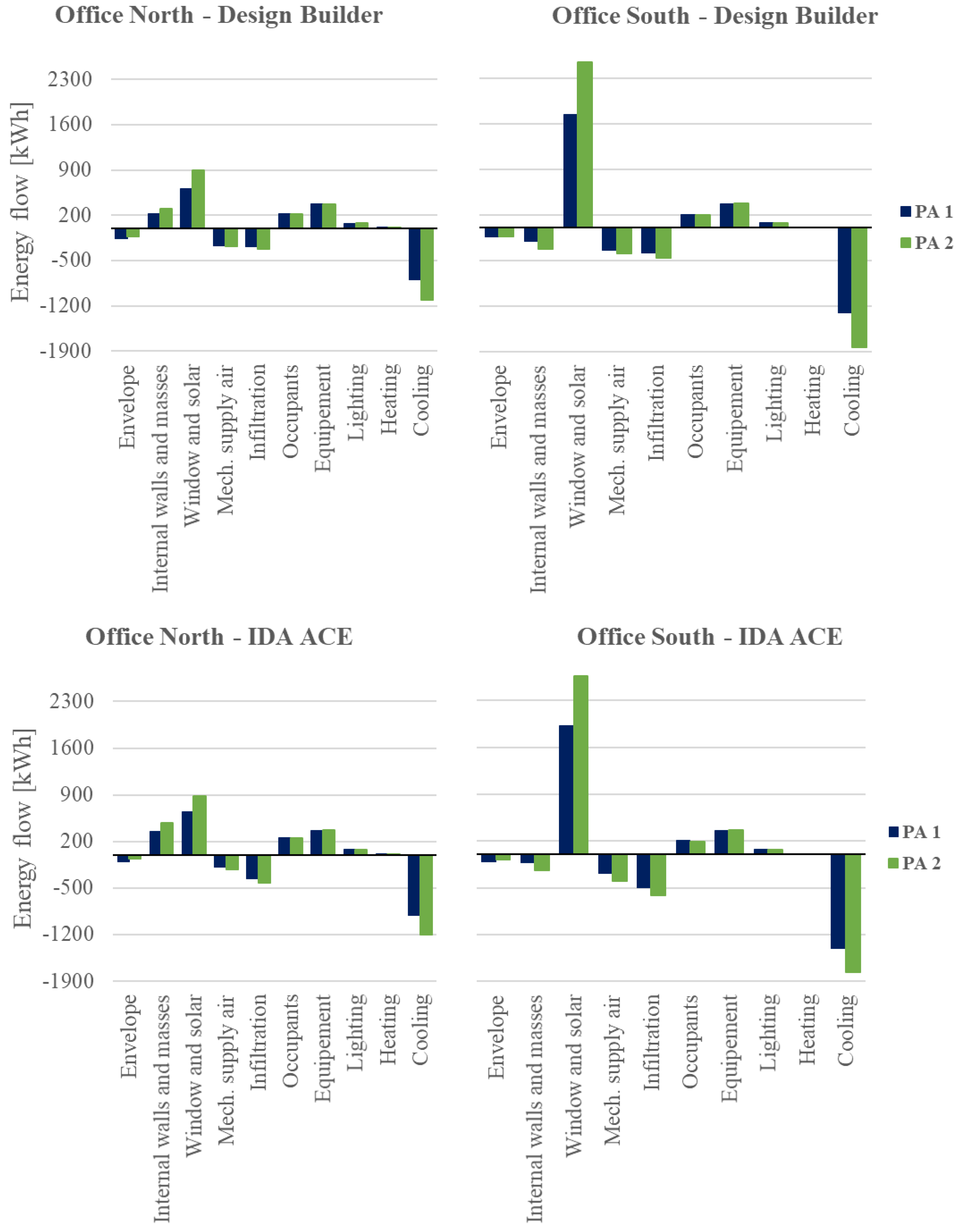These different approaches could explain the reason for the different operative temperature trends and the energy flows.

3.2.3. Delivered Energy

Figure 6 shows the yearly values of delivered energy for heating and cooling per square meter for each simulation.

Table 5. Difference percentage of annual delivered energy (ΔC: cooling difference; ΔH: heating difference) between scenario 1 (small window) and 2 (large window), calculated with Equations (10) and (11), and between Design Builder and IDA ICE, calculated with Equations (13) and (14).

Software	Simulation	Comparison
		Scenario 1 vs. Scenario 2		Design Builder vs. IDA ICE
		ΔC (%)	ΔH (%)	ΔW (%)	ΔS (%)
Design Builder	CPH 1	8	−6	0	−4
	CPH 2			0	0
	PA 1	22	0	0	0
	PA 2			−4	0
IDA ICE	CPH 1	8	−4
	CPH 2
	PA 1	19	0
	PA 2

summarizes the percentage differences in the heating/cooling energy use calculated with Equations (10) and (11).

As expected, wider transparent walls increase the energy required for cooling and decrease the energy for heating. The percentage differences predicted by both tools are similar except for heating in Copenhagen (highlighted in bold in Table 5). In this case, the percentage difference exhibited by Design Builder is almost twice that of IDA ICE (6% instead of 4%); however, these values are negligible. In cooling mode, the differences remain small for Copenhagen but increase for Palermo due to the higher radiative load.

The comparison between the operative temperature and delivered energy trends reveals that the decrease in the energy for heating for the second scenario does not result in significant variations in the percentage of operative temperature values higher than 20 °C. Similarly, the increase of cooling due to the increased solar radiation in summer does not result in more time in operative temperatures below 26 °C. These phenomena are probably due to the inability of the HVAC system to keep/control acceptable thermal comfort conditions.

3.3. First Scenario (Small Window) Design Builder vs. IDA ICE

3.3.1. Temperatures

The agreement between the two simulation tools in evaluating the thermo-hygrometric conditions has been expressed in terms of the percentage of the time that the temperature difference predicted by the two software falls into a specific condition (e.g., Δt ≤ 0.5 °C, 0.5 °C < Δt ≤ 1.0 °C; 1.0 °C < Δt ≤ 2.0 °C and Δt > 2.0 °C) according to Equation (8).

Table 6. Percentage of the time that the difference between the temperature values predicted by Design Builder and IDA ICE Δt (in °C) falls into a specific condition. CPH 1: Copenhagen/scenario 1, CPH 2: Copenhagen/scenario 2, PA 1: Palermo/scenario 1, PA 2: Palermo/scenario 2.

Condition	Scenario	North Office	South Office	Scenario	North Office	South Office
	CPH 1	Operative temperature		PA 1	Operative temperature
Δt ≤ 0.5		82	83		67	53
0.5 < Δt ≤ 1.0		11	11		12	10
1.0 < Δt ≤ 2.0		7	6		19	21
Δt > 2.0		0	0		2	16
		Mean radiant temperature			Mean radiant temperature
Δt ≤ 0.5		34	50		66	47
0.5 < Δt ≤ 1.0		36	32		10	22
1.0 < Δt ≤ 2.0		30	18		21	19
Δt > 2.0		0	0		3	12
		Air temperature			Air temperature
Δt ≤ 0.5		32	47		59	39
0.5 < Δt ≤ 1.0		28	29		20	18
1.0 < Δt ≤ 2.0		38	23		19	23
Δt > 2.0		2	1		2	20
	CPH 2	Operative temperature		PA 2	Operative temperature
Δt ≤ 0.5		91	78		53	38
0.5 < Δt ≤ 1.0		4	10		11	10
1.0 < Δt ≤ 2.0		4	9		29	18
Δt > 2.0		1	3		7	34
		Mean radiant temperature			Mean radiant temperature
Δt ≤ 0.5		47	47		51	31
0.5 < Δt ≤ 1.0		22	33		18	21
1.0 < Δt ≤ 2.0		30	17		26	23
Δt > 2.0		1	3		5	25
		Air temperature			Air temperature
Δt ≤ 0.5		43	42		45	22
0.5 < Δt ≤ 1.0		19	28		17	16
1.0 < Δt ≤ 2.0		35	25		26	21
Δt > 2.0		3	5		12	41

summarizes the obtained results for the operative temperature, the air temperature, and the mean radiant temperature for both climates in the two offices. The behaviour of the two simulation tools seems to be affected by the outdoor climatic conditions. Notably, the operative temperature difference in Copenhagen is less than 1.0 °C (more than 2.0 °C) for more than 90% (less than 3%) of the time. The agreement for the mean radiant temperature is slightly worse in both configurations (the time percentage with Δt ≤ 1.0 °C varies from 70 to 82%).

Due to the higher solar load, the temperature values predicted for Palermo by the investigated tools are farther away. More specifically, Δt values less than 0.5 °C occur in less than 67% (53%) of the time for the north (south) office in the case of scenario 1. In addition, time percentages with Δt values higher than 2.0 °C occur in 16% (20%) of operative temperatures (air temperature) in the worst case (south office).

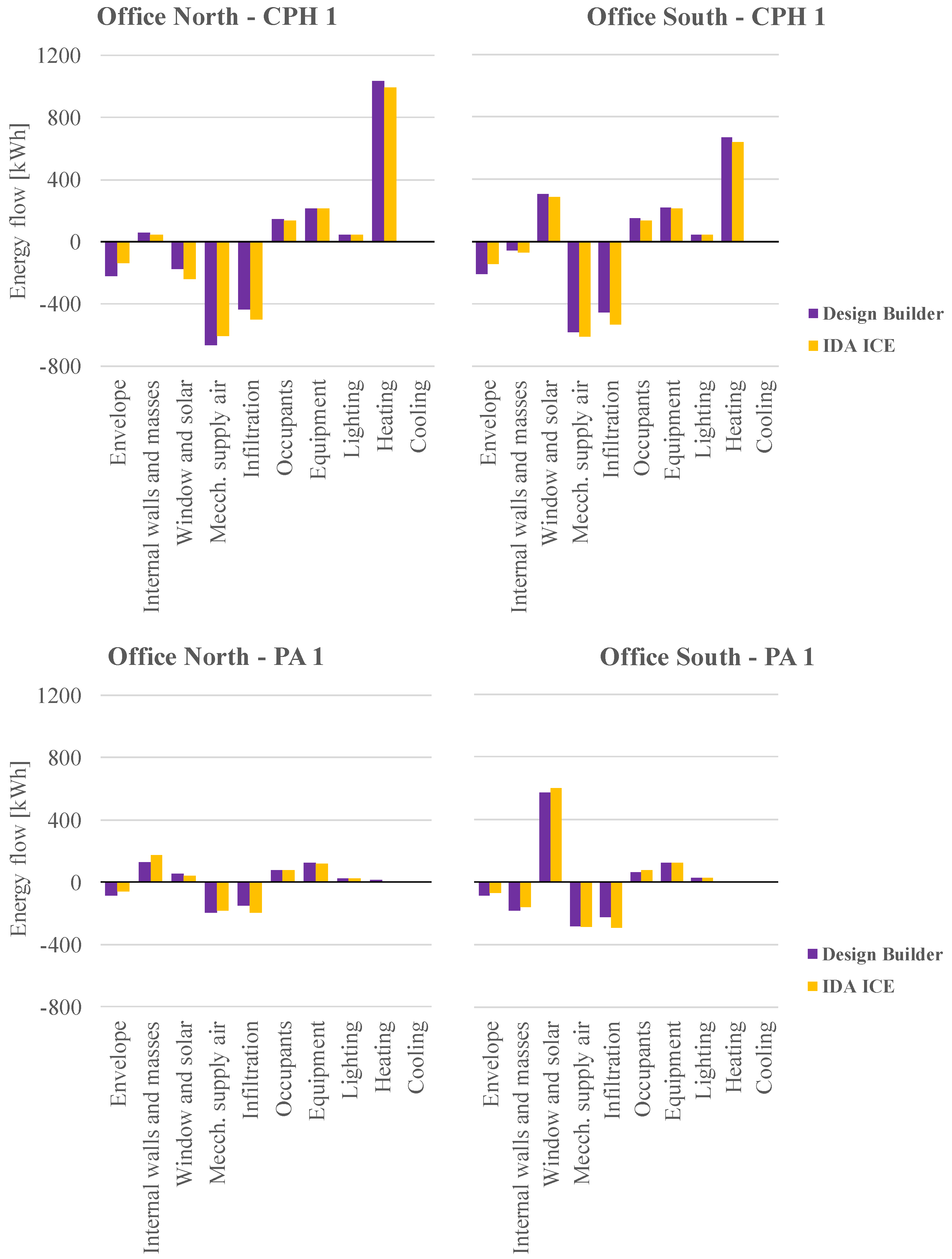
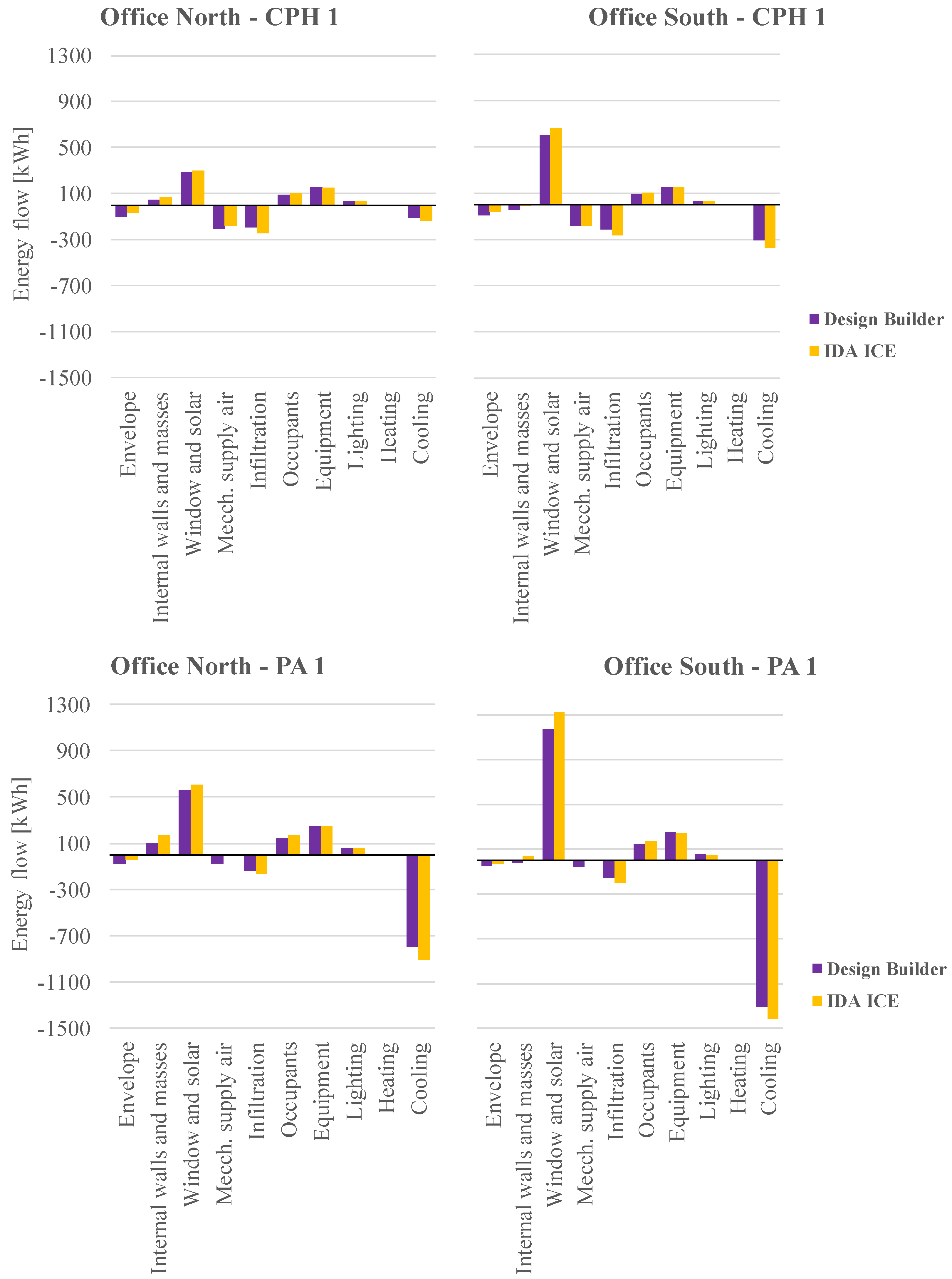
3.3.2. Energy Flows

The comparison between Design Builder and IDA ICE in terms of energy flows for each building component has been carried out on a seasonal basis. Figure 7 and Figure 8 report the thermal energy flows predicted in the first scenario during the two seasons.

The differences in energy flows, calculated with Equation (12), are generally negligible during winter and do not exceed 10%. During summer, the differences are 38% (16%) for “window and solar” in Copenhagen (Palermo) in the south office and 17% (12%) and 40% (11%) for “cooling” in Copenhagen (Palermo) for the north office and south office, respectively. Such an increase in summer finds a plausible explanation in the different approaches to modelling the radiation absorbed by the window system.

During summer, Copenhagen shows a high difference in percentages in the case of the components “internal walls and masses” (15% for the north office and 20% for the south office) and “envelope” (21% for the north office and 18% for the south office). This occurrence could be due to the calculation method of the U-value used by the two simulation tools.

However, to confirm this hypothesis, more investigations are required.

3.3.3. Delivered Energy

Table 5 shows the percentage of difference of the annual heating/cooling energy use per square meter compared to the overall energy use and calculated with Equations (13) and (14). The obtained results demonstrate a good agreement between the predicted overall energy use for heating and cooling with negligible differences (less than 4%). This behaviour also agrees with previous investigations [11], which revealed less than 14–16% difference between values.

3.4. Second Scenario (Large Windows) Design Builder vs. IDA ICE

3.4.1. Temperatures

The data in Table 6 prove that the agreement between the two simulation engines worsens for climatic conditions characterized by high solar loads. More specifically, as far as the operative temperature is concerned, the percentage of time with Δt ≤ 0.5 °C decreases from 67% to 53% (from 53 to 38%) for the north (south) office in Palermo. In addition, the percentage of time with Δt > 2.0 °C increases from 2% to 7% (from 16 to 34%) for the north (south) office. The air temperature (from 20 to 41%) and the mean radiant temperature (from 12 to 25%) also exhibit similar trends in the south office for the percentage of time with Δt > 2.0 °C.

Consequently, meaningful differences can occur when evaluating the thermal comfort conditions through the PMV. This is because the measurement errors are consistent with the required accuracy recommended by ISO 7726 [51] (e.g., ±0.5 °C for air temperature and ±2.0 °C for mean radiant temperature) and result in PMV errors of above two decimal points [52,53,54,55,56]).

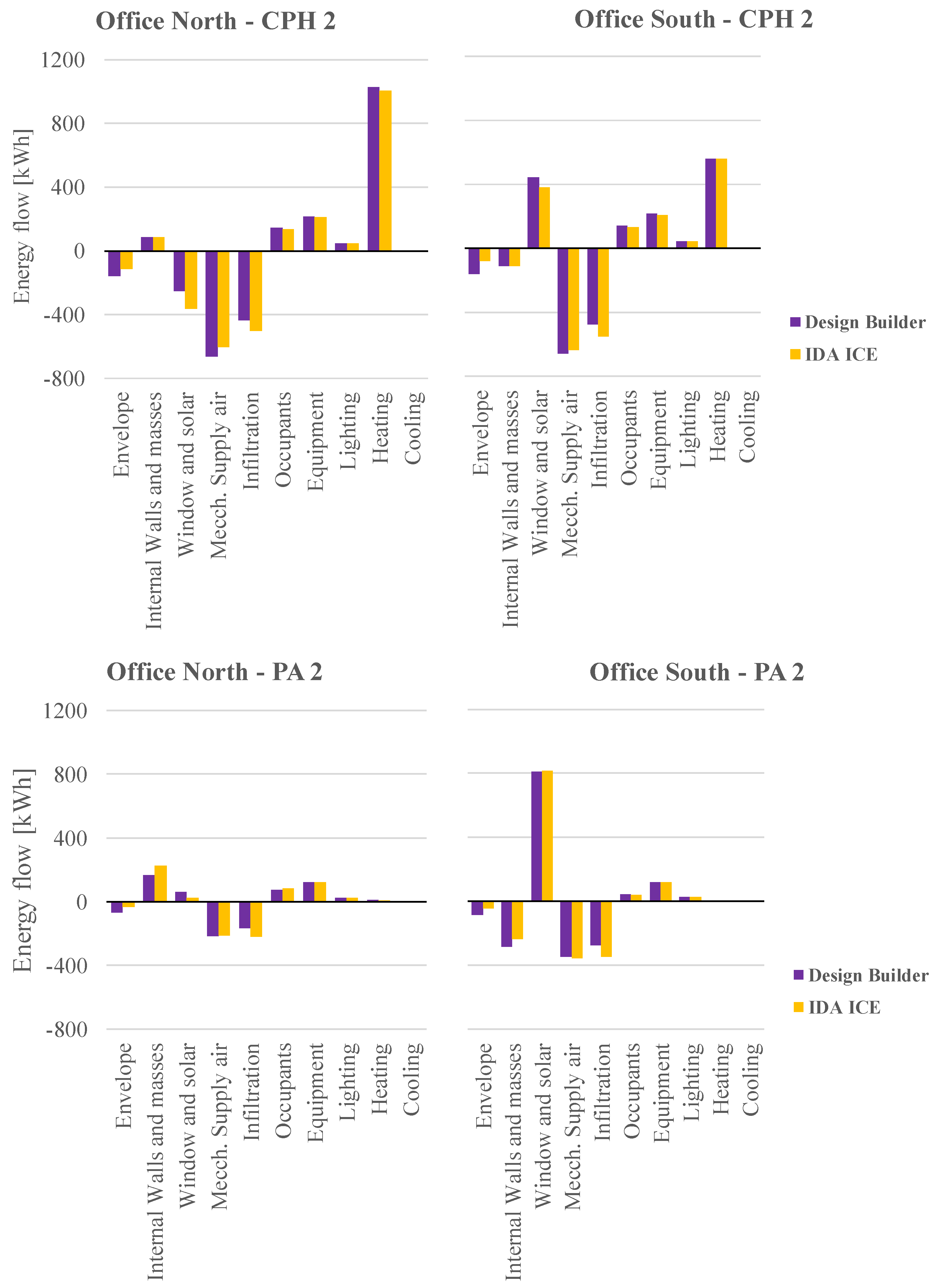
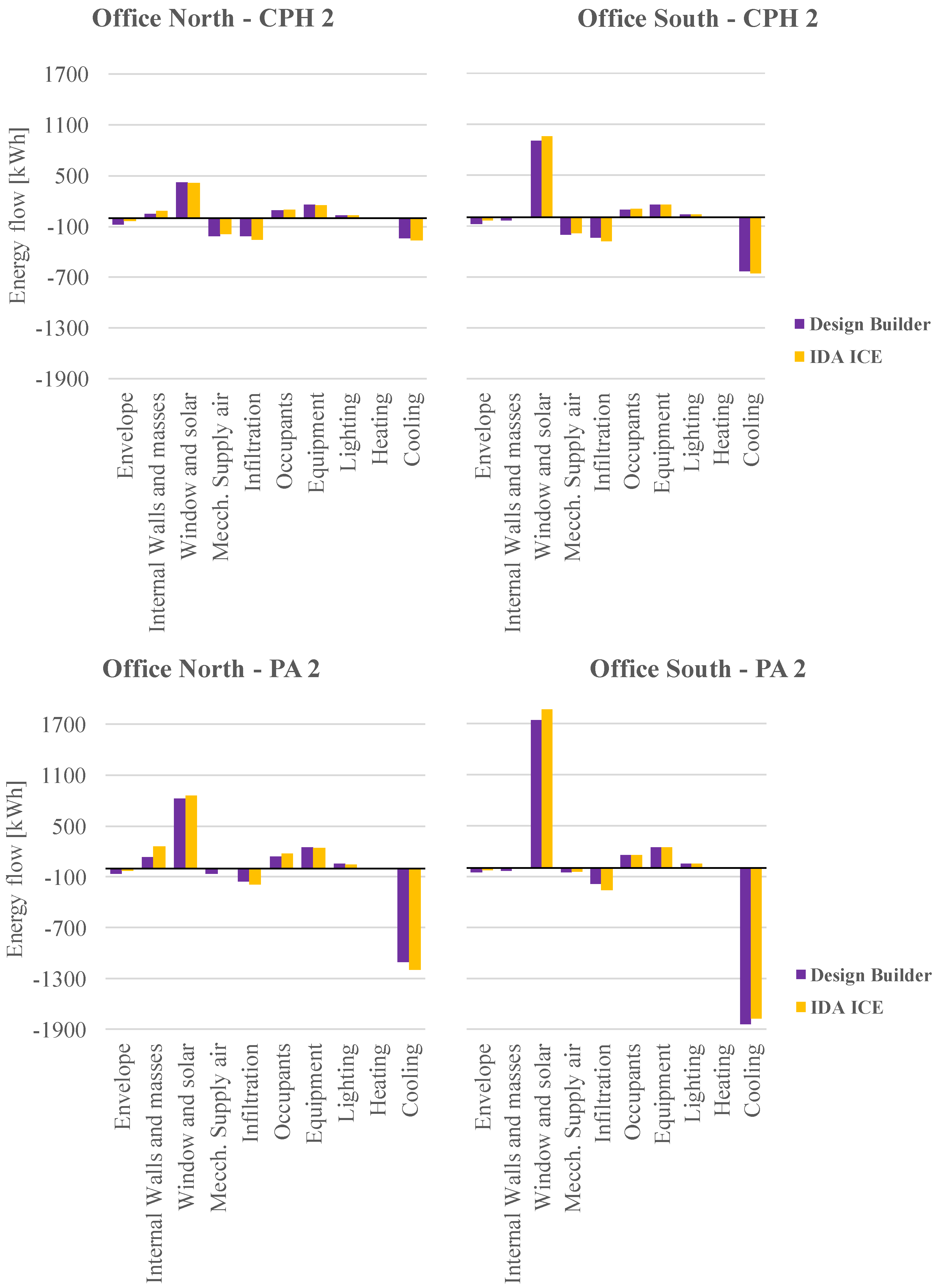
3.4.2. Energy Flows

Figure 9 and Figure 10 show the thermal energy flows predicted in the second scenario during the two seasons.

As for scenario 1, there are no significant differences in the predicted energy values during winter. The highest value (around 11%) occurred for the “internal walls and masses” component. As observed above, a plausible explanation could be the different ways for calculating the U-value. The difference found for the “window and solar” contributions (17% and 11% for Copenhagen and Palermo, respectively) in the south office could be due to the different ways that solar radiation through windows is dealt with.

3.4.3. Delivered Energy

Table 5 shows the percentage of difference in the annual heating/cooling energy use per square meter calculated with Equations (13) and (14). As observed above, the obtained results reveal a good agreement between Design Builder and IDA ICE, with overall energy use for heating and cooling being very close to each other, and with a maximum difference percentage equal to 4%.

4. Conclusions

Building Energy Performance Simulation tools with specific modular structures, such as Design Builder and IDA ICE, are irreplaceable instruments for energy calculations and the evaluation of thermal comfort. However, a reliable prediction of the building behaviour requires an in-depth analysis of the input data that is used for the modelling that often require a different approach (and different level of experience) depending on the tool used.

The first part of the present investigation has focused on this issue. Then, the paper compared the energy use and thermal comfort conditions predicted by the two engines in different climates and building scenarios.

The main results can be summarized as follows.

• Creating the same building model using different tools requires significant effort to define input data. Most notably, we have shown that using the same input data set is not always possible. Consequently, it is impossible to evaluate how any slight variation of the input data can affect the output for the same building model. For instance, the U-values obtained by the two tools can differ above 12% for the same building typology (e.g., used materials, thicknesses values).
• In agreement with previous investigations that focused on the energy use predicted by different simulation tools, Design Builder and IDA ICE do not exhibit significant differences (<4%) in the yearly energy use of the building. Some differences (>10%) occur for the energy flows related to specific components (e.g., internal walls and masses, windows, and solar components during summer). A plausible explanation could be the different ways to calculate the U-value and consider the solar radiation absorbed by the glazing walls.
• The most significant differences when using the two tools are related to the operative temperatures rather than the energy delivered for the identical building model.
• IDA ICE exhibits a more noticeable temperature variation that affects the overall energy used for cooling. Consequently, cooling is sometimes required in winter to have better thermal comfort conditions. The effects are most significant for a warmer climate (Palermo) and in the presence of wide glazing walls. In this case, the operative temperature differences obtained by the two tools exceed 2.0 °C one-third of the time. A plausible explanation could be the different ways of evaluating the U-values and the solar radiation through the windows. However, the differences in evaluating thermal comfort conditions through the PMV require further investigation.
• Using a simple HVAC system in Design Builder does not allow the user to define a range of thermal comfort, but it only gives the option to define the set point temperature for the heating and cooling system. Given this, the HVAC system provides heating/cooling when the operative temperature is below/above the desired temperature set point. When this does not happen, the reason could be an insufficient capacity/control of the system plant or a free-running condition, as occurred in simulations for Palermo. The differences in the results could be relevant in terms of design choices or a tender offer.

The obtained results show how necessary the knowledge of these tools is to maximize their potentialities and reduce the impact of their limitations. On the one hand, BEPS software is a powerful tool that is able to perform the energy design and evaluate the indoor climate at a detailed time step. On the other hand, it can deviate from the real behaviour of the building if users (e.g., designers and researchers) need to be more skilled in dealing with boundary conditions and the different algorithms at the base of the calculation. In a nutshell, it is necessary to correctly manage the multiple input data and have a critical approach to the analyses of results, thereby not exclusively relying on the software outcomes.

To highlight further critical issues in data preparation, we will extend the analysis to different building typologies and architectural layouts. In addition, we will investigate the different ways to deal with heat transfer by radiation. Finally, numerical outputs from the present research will be validated by monitoring the indoor thermo-hygrometric parameters in a reference building.

References

- Vijayavenkataraman, S.; Iniyan, S.; Goic, R. A review of climate change, mitigation and adaptation. Renew. Sustain. Energy Rev. 2012, 16, 878–897. [Google Scholar] [CrossRef]
- Buildings—Tracking Report September 2022; International Energy Agency: Paris, France, 2022; Available online: https://www.iea.org/reports/buildings (accessed on 27 December 2022).
- European Parliament. Directive (EU) 2018/844 of the European Parliament and of the Council of 30 May 2018 amending Directive 2010/31/EU on the energy performance of buildings and Directive 2012/27/EU on energy efficiency. Off. J. Eur. Union 2018, 156, 75–91. [Google Scholar]
- Artola, I.; Rademaekers, K.; Williams, R.; Yearwood, J. Boosting Building Renovation: What Potential and Value for Europe; Study for the iTRE Committee, Commissioned by DG for Internal Policies Policy Department A; European Parliament: Brussels, Belgium, 2016; Volume 72. [Google Scholar]
- D’Agostino, D.; Mazzarella, L. What is a Nearly zero energy building? Overview, implementation and comparison of definitions. J. Build. Eng. 2019, 21, 200–212. [Google Scholar] [CrossRef]
- Hong, T.; Langevin, J.; Sun, K. Building simulation: Ten challenges. Build. Simul. 2018, 11, 871–898. [Google Scholar] [CrossRef] [Green Version]
- EN 16798-2; Energy Performance of Buildings—Ventilation for Buildings—Part 2: Interpretation of the Requirements in EN 16798-1—Indoor Environmental Input Parameters for Design and Assessment of Energy Performance of Buildings Addressing Indoor Air Quality, Thermal Environment, Lighting and Acoustics—Module M1-6. European Committee for Standardization: Brussels, Belgium, 2019.
- EN 16798-1; Indoor Environmental Input Parameters for Design and Assessment of Energy Performance of Buildings Addressing Indoor Air Quality, Thermal Environment, Lighting and Acoustics-Module M1-6. European Committee for Standardization: Brussels, Belgium, 2019.
- Santos-Herrero, J.M.; Lopez-Guede, J.M.; Flores-Abascal, I. Modeling, simulation and control tools for nZEB: A state-of-the-art review. Renew. Sustain. Energy Rev. 2021, 142, 110851. [Google Scholar] [CrossRef]
- Baglivo, C.; Congedo, P.; Di Cataldo, M.; Coluccia, L.; D’Agostino, D. Envelope design optimization by thermal modelling of a building in a warm climate. Energies 2017, 10, 1808. [Google Scholar] [CrossRef] [Green Version]
- Hoyt, T.; Arens, E.; Zhang, H. Extending air temperature setpoints: Simulated energy savings and design considerations for new and retrofit buildings. Build. Environ. 2015, 88, 89–96. [Google Scholar] [CrossRef] [Green Version]
- Hong, T.; Chena, Y.; Luo, X.; Luo, N.; Lee, S.H. Ten questions on urban building energy modelling. Build. Environ. 2020, 168, 106508. [Google Scholar] [CrossRef] [Green Version]
- Wang, C.; Ferrando, M.; Causone, F.; Jin, X.; Zhou, X.; Shi, X. Data acquisition for urban building energy modeling: A review. Build. Environ. 2022, 217, 109056. [Google Scholar] [CrossRef]
- EnergyPlus Building Energy Simulation Program of U.S. Department of Energy’s (DOE) Building Technologies Office (BTO) and Managed by the National Renewable Energy Laboratory (NREL). Available online: https://energyplus.net/ (accessed on 10 December 2022).
- DesignBuilder Software Ltd. Stroud House Russell Street Stroud, Gloucs GL5 3AN, UK. Available online: https://designbuilder.co.uk/ (accessed on 4 January 2023).
- IDA Indoor Climate and Energy. EQUA Simulation AB Råsundavägen 100, 169 57 Solna, Sweden. Available online: https://www.equa.se/en/ida-ice/ (accessed on 10 December 2022).
- ASHRAE 140; Standard Method of Test for the Evaluation of Building Energy Analysis Computer Programs. American Society of Heating, Refrigerating, and Air-Conditioning Engineers, Inc.: Atlanta, GA, USA, 2014.
- EN 15255; Energy Performance of Buildings—Sensible Room Cooling Load Calculation—General Criteria and Validation Procedures. European Committee for Standardization: Brussels, Belgium, 2007.
- EN 15265; Energy Performance of Buildings—Calculation of Energy Needs for Space Heating and Cooling Using Dynamic Methods—General Criteria and Validation Procedures. European Committee for Standardization: Brussels, Belgium, 2007.
- EN 13791; Thermal Performance of Buildings—Calculation of Internal Temperatures of a Room in Summer without Mechanical Cooling—General Criteria and Validation Procedures. European Committee for Standardization: Brussels, Belgium, 2012.
- Lolli, N.; Brozovsky, J.; Nocente, A.; Grynning, S. Temperature and thermal comfort in office spaces: Measurements vs. simulations. In Proceedings of the 16th IBPSA Conference, Rome, Italy, 2–4 September 2019; pp. 1849–1858. [Google Scholar] [CrossRef]
- Yu, J.; Chang, W.-S.; Dong, Y. Building Energy Prediction Models and Related Uncertainties: A Review. Buildings 2022, 12, 1284. [Google Scholar] [CrossRef]
- van Dronkelaar, C.; Dowson, M.; Spataru, C.; Mumovic, D. A Review of the Regulatory Energy Performance Gap and Its Underlying Causes in Non-domestic Buildings. Front. Mech. Eng. 2016, 1, 17. [Google Scholar] [CrossRef] [Green Version]
- van den Brom, P.; Meijer, A.; Visscher, H. Performance gaps in energy consumption: Household groups and building characteristics. Build. Res. Inf. 2018, 46, 54–70. [Google Scholar] [CrossRef] [Green Version]
- Laskari, M.; de Masi, R.-F.; Karatasou, S.; Santamouris, M.; Assimakopoulos, M.-N. On the impact of user behaviour on heating energy consumption and indoor temperature in residential buildings. Energy Build. 2022, 255, 111657. [Google Scholar] [CrossRef]
- Huerto-Cardenas, H.E.; Leonforte, F.; Aste, N.; Del Pero, C.; Evola, G.; Costanzo, V.; Lucchi, E. Validation of dynamic hygrothermal simulation models for historical buildings: State of the art, research challenges and recommendations. Energy Build. 2020, 180, 107081. [Google Scholar] [CrossRef]
- Crawley, D.B.; Hand, J.W.; Kummert, M.; Griffith, B.T. Contrasting the capabilities of building energy performance simulation programs. Build. Environ. 2008, 43, 661–673. [Google Scholar] [CrossRef] [Green Version]
- Sousa, J. Energy simulation software for buildings: Review and comparison. Inf. Technol. Energy Appl. 2012, 6–7. Available online: https://ceur-ws.org/Vol-923/paper08.pdf (accessed on 4 January 2023).
- Mazzeo, D.; Matera, N.; Cornaro, C.; Oliveti, G.; Romagnoni, P.; De Santoli, L. EnergyPlus, IDA ICE and TRNSYS predictive simulation accuracy for building thermal behaviour evaluation by using an experimental campaign in solar test boxes with and without a PCM module. Energy Build. 2020, 212, 109812. [Google Scholar] [CrossRef]
- Vadiee, A.; Dodoo, A.; Gustavsson, L. A Comparison Between Four Dynamic Energy Modeling Tools for Simulation of Space Heating Demand of Buildings. In CCC 2018: Cold Climate HVAC 2018; Springer Proceedings in Energy; Johansson, D., Bagge, H., Wahlström, Å., Eds.; Springer: Cham, Switzerland. [CrossRef]
- Johari, F.; Nilsson, A.; Åberg, M.; Widén, J. Towards Urban Building Energy Modelling: A Comparison of Available Tools. In Proceedings of the ECEEE 2019 Summer Study on Energy Efficiency: Is Efficient Sufficient? Hyères, France, 3–8 June 2019; pp. 1515–1524. [Google Scholar]
- Mirsadeghi, M.; Costola, D.; Blocken, B.; Hensen, J.L. Review of external convective heat transfer coefficient models in building energy simulation programs: Implementation and uncertainty. Appl. Therm. Eng. 2013, 56, 134–151. [Google Scholar] [CrossRef]
- Gelesz, A.; Lucchino, E.C.; Goia, F.; Serra, V.; Reith, A. Characteristics that matter in a climate façade: A sensitivity analysis with building energy simulation tools. Energy Build. 2020, 229, 110467. [Google Scholar] [CrossRef]
- Zhu, D.; Hong, T.; Yan, D.; Wang, C.A. A detailed loads comparison of three building energy modeling programs: EnergyPlus, DeST and DOE-2.1 E. Build. Simul. 2013, 6, 323–335. [Google Scholar] [CrossRef]
- Kottek, M.; Grieser, J.; Beck, C.; Rudolf, B.; Rubel, F. World Map of the Köppen-Geiger climate classification updated. Meteorol. Z. 2006, 15, 259–263. [Google Scholar] [CrossRef]
- Weather Data Available in EnergyPlus. Available online: https://energyplus.net/weather/ (accessed on 4 January 2023).
- Big Ladder Software LLC. Elements for Windows (Ver. 1.06). Available online: https://download.bigladdersoftware.com/?ref=elements-latest-win (accessed on 4 January 2023).
- Olesen, B.W.; Dossi, F.C. Operation and control of activated slab heating and cooling systems. In Proceedings of the CIB World Building Congress 2004: Building for the Future, Toronto, ON, Canada, 2–7 May 2004. [Google Scholar]
- WINDOW Computer Program Developed at Lawrence Berkeley National Laboratory (LBNL). Available online: https://windows.lbl.gov/sites/default/files/software/WINDOW/WINDOW7UserManual.pdf (accessed on 4 January 2023).
- Kolarik, J.; Toftum, J.; Olesen, B.W.; Jensen, K.L. Simulation of energy use, human thermal comfort and office work performance in buildings with moderately drifting operative temperatures. Energy Build. 2011, 43, 2988–2997. [Google Scholar] [CrossRef] [Green Version]
- Decree by The President of the Republic 16 Aprile 2013 n. 74, Regolamento Recante Norme per la Progettazione, L’installazione, L’esercizio e la Manutenzione degli Impianti Termici Degli Edifici ai Fini del Contenimento dei Consumi di Energia, in Attuazione dell’art. 4, Comma 4, Della Legge 9 Gennaio 1991 n. 10. Gazzetta Ufficiale n. del 149 del 27 giugno 2013; Presidenza della Repubblica Italiana, Rome, Italy 2013. Available online: https://www.gazzettaufficiale.it/eli/id/2013/06/27/13G00114/sg (accessed on 7 January 2023).
- Standalone DesignBuilder Results Viewer. Available online: https://designbuilder.co.uk/helpv5.5/#ResultsProcessor.htm?Highlight=results (accessed on 10 December 2022).
- Auxiliary Energy data in DesignBuilder. Available online: https://designbuilder.co.uk/helpv5.5/#Auxiliary_Energy.htm?Highlight=Auxiliary%20Energy (accessed on 10 December 2022).
- ISO 8996; Ergonomics of the Thermal Environment—Determination of Metabolic Rate. International Standardization Organization: Geneva, Switzerland, 2022.
- Du Bois, D.; Dubois, E. A formula to estimate the approximate surface area if height and weight be known. Arch. Intern. Med. 1916, 17, 863–871. [Google Scholar] [CrossRef] [Green Version]
- ISO 7730; Ergonomics of the Thermal Environment—Analytical Determination and Interpretation of Thermal Comfort Using Calculation of the PMV and PPD Indices and Local Thermal Comfort Criteria. European Standardization Organization: Brussels, Belgium, 2005.
- General Lighting in DesignBuilder. Available online: https://designbuilder.co.uk/helpv5.5/#_General_lighting.htm?Highlight=radiant%20fraction (accessed on 10 December 2022).
- ISO 6946; Building Components and Building Elements—Thermal Resistance and Thermal Transmittance—Calculation Method. International Standardization Organization: Geneva, Switzerland, 2018.
- EQUA Simulation AB, Energy Modeling in IDA ICE according to ASHRAE 90.1-2010. Available online: http://www.equaonline.com/iceuser/pdf/ASHRAE_90.1_Extension_v2010.pdf (accessed on 10 December 2022).
- ASHRAE 90.1; Energy Standard for Buildings Except Low-Rise Residential Buildings. American Society of Heating, Refrigerating, and Air-Conditioning Engineers, Inc.: Atlanta, GA, USA, 2019.
- ISO 7726; Ergonomics of the Thermal Environment—Instruments for Measuring Physical Quantities. International Standardization Organization: Geneva, Switzerland, 2002.
- Dell’Isola, M.; Frattolillo, A.; Palella, B.I.; Riccio, G. Influence of Measurement Uncertainties on the Thermal Environment Assessment. Int. J. Thermophys. 2012, 33, 1616–1632. [Google Scholar] [CrossRef]
- d’Ambrosio Alfano, F.R.; Palella, B.I.; Riccio, G. The Role of Measurement Accuracy on the Thermal Environment Assessment by means of PMV Index. Build. Environ. 2011, 46, 1361–1369. [Google Scholar] [CrossRef]
- Palella, B.I.; Quaranta, F.; Riccio, G. On the management and prevention of heat stress for crews onboard ships. Ocean Eng. 2016, 112, 277–286. [Google Scholar] [CrossRef]
- d’Ambrosio Alfano, F.R.; Olesen, B.W.; Pepe, D.; Palella, B.I.; Riccio, G. Fifty Years of PMV Model: Reliability, Implementation and Design of Software for Its Calculation. Atmosphere 2020, 11, 49. [Google Scholar] [CrossRef] [Green Version]
- d’Ambrosio Alfano, F.R.; Ficco, G.; Frattolillo, A.; Palella, B.I.; Riccio, G. Mean Radiant Temperature Measurements through Small Black Globes under Forced Convection Conditions. Atmosphere 2021, 12, 621. [Google Scholar] [CrossRef]