Impact of Superconducting Cables on a DC Railway Network

Abstract

The Société Nationale des Chemins de fer Français (SNCF) is facing a significant challenge to meet the growth in rail traffic while maintaining continuous service, particularly in densely populated areas such as Paris. To tackle this challenge, the SNCF has implemented several electrification projects. These projects aim to reduce line losses and decrease voltage drops on the railway network. Amongst the possible technological choices, high temperature superconductor (HTS) cables have been evaluated, since they offer greater energy density at lower electrical losses than conventional cables. This feature is advantageous in order to transmit more electrical energy at a lesser footprint than conventional cable, therefore avoiding costly modifications of the existing infrastructures. In the present work, the electromagnetic response of two HTS cables topologies, unipolar and bipolar, was analyzed, and their impact on a direct current (DC) railway network under load was assessed. A commercial finite element (FE) software, COMSOL Multiphysics, was used to carry out a detailed FE model that accounts for the non-linearity of the electrical resistivity ρ (J, B, θ) of the superconducting cable. This FE model was coupled with a lumped-parameter circuit model of the railway network, which is particularly suited for transient simulations considering train motion. Based on a case study representing a portion of the Parisian railway network, it was found that the insertion of a superconducting cable can result in a reduction of electrical losses by 60% compared to conventional cable as well as an 8.6% reduction in the total electrical consumption of the traction network.

1. Introduction

High-temperature superconductors (HTS) are slowly replacing conventional conductors in specific power applications demanding high power density. They have gained traction as they also present negligible losses in AC, therefore allowing for the construction of better-performing power devices that can provide uninterrupted transmission of electrical energy [1]. In this context, superconducting cables could replace conventional cables as a means to transmit electricity over long distances with lower losses [2,3]. They can also be used to power large-scale instruments such as accelerators, reducing power losses and improving overall system performance. Superconducting machines, such as motors and generators, are generally more efficient and compact than their conventional counterparts for the same power output [4,5]. They have already been considered in a variety of applications requiring high power and high efficiency, such as power grids, wind power, ships, and airplanes, amongst others. Superconducting transformers also have some advantages over traditional iron-core transformers: they are more efficient, can include a current limiting capability, and can be designed more compactly [6,7,8]. In summary, the use of superconducting power devices can lead to a significant reduction in energy consumption and energy-related costs as well as an improvement in the performance and efficiency of electrical systems.

French freight and passenger rail transports rely heavily on DC electrical networks of less than 1.5 kV for historical and geographical reasons [9]. The traction power network is indeed built for relatively low voltage to distribute high current. In France, the length of direct current lines under 1.5 kV is equal to 5904 km, or about 1/4th of the national railway electrification [10]. Often, both their infrastructure and architecture have to evolve in order to cope with the increase in energy consumption while complying with the reduction of CO₂ emissions following the evermore constraining environmental reforms [11]. In a 1.5 kV low-voltage DC grid, the distance between substations (SS) is of the order of a few tens of kilometers [12], and the section of the overhead conductors can be as large as 1000 mm² [13]. In order to avoid consequent voltage drops, several solutions have already been considered and tried out. The main ones involve the reduction of the distance between the substations and/or the increase of the cross section of the overhead lines. In both cases, either a transformer substation near the location of the demand, whose installation in a densely populated area would impose new civil and electrical engineering developments, or an increase of the mechanical infrastructure of the overhead line, already heavy, would be necessary. These options convey additional costs which do not offset the gain from the voltage drop. In order to avoid additional investment in infrastructure while addressing the voltage drop by reducing the electrical losses along the line in restrained environment, an appealing technological solution is based on the installation of a superconducting power cable. The idea is to benefit from the new developments in commercial high-temperature superconducting (HTS) tapes referred to as second generation or 2G while providing a high current density at no loss in DC regime with a better mechanical strength. Thus, a typical commercially available single 2G superconducting tape has an average current density of about 400 A/mm² at liquid nitrogen (77 K) [14], which is 400 times higher than the 1 A/mm² of a copper conductor according to DIN43671. Besides its ability to transmit a very high energy density, there are no electrical losses in the superconductor in DC conditions. Due to the electrical advantages of 2G-HTS tapes over conventional copper wire, DC cables made of those tapes have been developed, built, and utilized in several international pilot and demonstration projects.

Figure 1 compiles several superconducting cable trials in recent years in order to test the reliability of superconducting cables, mostly in power grids but also in traction networks [15,16,17,18,19,20,21,22,23]. According to our knowledge, Japan was the first country to have installed a superconducting cable in a railway network with a 31 m-long prototype tested at 10 V and a 310 m-long cable installed in Tokyo in 2016. It is a bipolar cable with a nominal current of 1 kA and consisting of two types of superconducting tapes; 78% are Bi2223 tapes and 22% are YBCO tapes [24]. In France, this technology is currently assessed by the SNCF as part of the “SuperRail” project aiming to install two 80 m-long superconducting cables on a commercial line near the Montparnasse station in Paris [25]. For this project, preliminary studies, presented in this work and relying on refined models of the superconducting cable, have been carried out in order to verify their performance in the traction network but also their impact on the latter. The studies are as follows: (1) quantitative evaluation of the benefits of using a superconducting cable over a conventional technology (energy consumption and voltage drop reduction) (2) estimation of the impact of the superconducting cable on three major components of the railway network, which are the substation, the traction line, and the train (energy gain). The first study specifically aims at estimating the cable losses in operation.

From the stand-point of modeling and simulation, the present work relies on past works simulating the railway network in dynamic regime for conventional technology on one hand [26,27,28,29,30] and the development of FE models to simulate superconducting cables on the second hand [31,32,33,34]. To date, there have been no attempts, at least to the best of the authors’ knowledge, to simulate in transient a superconducting cable in a traction network as proposed hereinafter. Past and current works reported in the literature have only considered the superconducting cable as a constant electrical resistance equal to zero [35], or in the best case scenario as a nonlinear resistance depending on current and temperature [36]. These simplified models can yield a good assessment of the total current flowing through the cable, but they are unsuitable for estimating the hysteresis and/or dynamic losses of a complicated structure as found in a superconducting cable made of various tapes connected in parallel stacked in layers on a metallic former. The present work provides the level of details needed to estimate the electrical losses with a high degree of accuracy using the latest electromagnetic models developed specifically for 2G-HTS technology [37]. The same electromagnetic detailed model yields the evolution of the impedance of the cable following the movements of the trains that can be used to feedback the circuit model of a traction line.

As mentioned previously, the objective of the present work is to evaluate quantitatively the electrical impact that a superconducting cable can have on a 1500 V DC railway network. The reference for defining the magnitude of this impact is given by considering a conventional cable against which two topologies of superconducting cable, unipolar and bipolar, are compared.

This paper is organized into eight sections. Following the general introduction, Section 2 describes the objective of the work, which was defined as part of the tasks conducted in the project SuperRail to assess the relevance of using superconducting cables to unclog the traction network at Montparnasse railway station. In the same section, the employed methodology is detailed. Section 3 details the two topologies and designs retained for the superconducting cables and introduces the cooling system. The same cooling system is used for both topologies of cables. The algorithm developed to dimension the system is found in [38]. This algorithm estimates the heat losses of the HTSC cable, the terminations, and the components of the cooling system. In the same section, the finite element (FE) model, developed to calculate the dynamic losses of the superconducting cables, is detailed. This model implements the T-A formulation of the Maxwell equations. This model takes into consideration the highly nonlinear behavior of the resistance of the superconductor via the power law E(J) relating the electric field along the superconductor E to its current density J. Details of the physics of the superconductor are considered via the Kim–Anderson relation. This relation expresses the dependence of the critical current density of the superconducting tape J_c with respect to the magnetic flux density B and its orientation (angle θ). Section 4 introduces the circuit model of the DC railway network (case study) and, in particular, its main components: the substations and the traction line whose impedances change over time due to the acceleration and deacceleration of the moving trains. Section 5 presents the co-simulation approach, i.e., the coupling of the portion of DC traction network modeled in Simulink and the FE model of the superconducting cable in COMSOL Multiphysics. Section 6 is an evaluation of the power consumption and voltage drop on the traction line for a constant train speed in a case study involving two substations connected to the power grid. Section 7 addresses a transient problem with two additional scenarios considering two speed profiles for two trains leaving two substations at the same time or at different times. These case studies provide a baseline to further studies considering different scenarios of operation of the traction line. A small Section 8 is dedicated to a brief discussion summarizing the work carried out in the paper followed by a conclusion presenting the substantial results.

2. Objective and Methodology

2.1. Objective

The objective was to develop a numerical tool to design superconducting cables, and then to study their feasibility and their advantages in a traction network. This requires the optimization of the whole superconducting cable and the railway network. On the one hand, the existing sizing algorithms in the literature require knowledge of the length of the superconducting cable. On the other hand, the length of the cable is the key variable for optimizing the superconducting cable in a railway network. In this paper, we size several cables with lengths ranging from 0.1 to 5 km in order to determine the optimal length to promote the benefits of inserting the superconducting cable in the railway network. Then, through a simulation of the whole, we discuss the advantages of the insertion of the superconducting cable in the railway network, having previously analyzed the reduction of the losses on the lines and the electric consumption of the system.

2.2. Methodology

Figure 2 shows a flowchart of the procedure followed in the present work. This procedure can be divided into four main steps.

The first step concerns the dimensioning of several cables according to a set of specifications and for different lengths, where the dimensioning algorithm presented in Figure 3 of Reference [38] is used. During this step, the optimal dimensions and parameters of the superconducting cable, including the necessary cryogenic infrastructure, are determined for each required length. The second step contains a model of the railway network. This concerns the modeling of the main elements of the network, in particular the substations, the trains, and the management of the impedance of the lines, in order to consider the displacement of the load according to time and space. The third step consists of coupling an FEM model where the parameters of the superconducting cables sized during Step 1 are used in an electrical model of the railway network built in Step 2. The end of the process consists of data processing to calculate the energy consumed by each installation, including the cable cooling system.

3. Design and Modeling of DC Superconducting Cable and Its Auxiliary Systems

3.1. Cable Topologies

In a DC railway network, two superconducting cable topologies may be considered: (1) unipolar or (2) bipolar. Figure 3a shows the insertion of a unipolar DC HTSC with only one positive pole. In this configuration, the current flows from the output of the AC/DC rectifier at a voltage of 1.5 kV to the injection point on the traction line. They contain a single pole to carry the current from the substation outlet to the injection point of the overhead line. Figure 3b shows a bipolar cable with two concentric positive and negative poles that provide the path for the direct and reverse currents. Out of the two topologies, unipolar is the technology considered the most reliable and the easiest to implement in the railway network, as it does not require any modifications of the existing network. However, the bipolar topology is expected to be the most effective solution to reduce the voltage drop on the traction line, as it provides a direct power return to the substation without passing through the dissipative rails (see Section 6). If the configuration assumes current return through the rails, the actual distribution of the current density in the rails can be determined, as proposed in [39,40]. Interestingly, the rails are also used to send electrical signals to detect the position of the train or the location of a fault from a distance. However, this functionality adds tremendous complexity to ensure a safe and reliable operation of the system with a bipolar superconducting cable. Indeed, when the train travels between the injection point and the point of connection to the substation, the electrical signals sent through the rails are short-circuited by the superconducting cable, whose impedance is much lower than that of the rails. Such functionality is not considered in the present work.

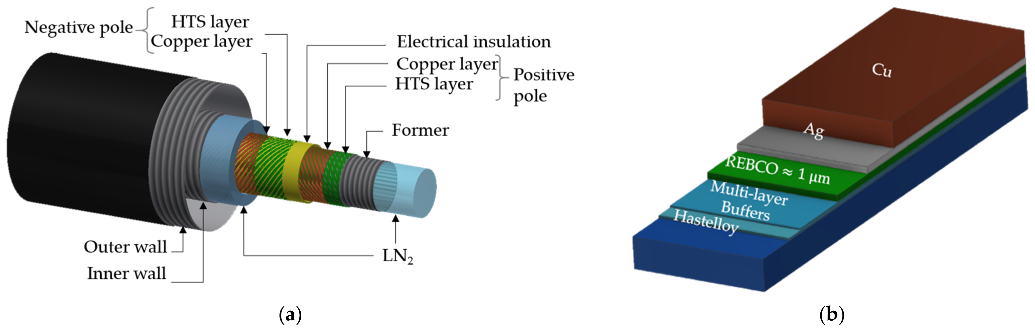
3.2. Design of the DC HTS Cables

The DC HTC cables are composed of several concentric layers of tape wound on a liquid nitrogen pipe (former) which cool the superconducting tapes to their operating temperature in the typical range of 68–78 K in order to maintain the nitrogen in a liquid state. Figure 4a shows a complete 3D view of a typical bipolar coaxial cable. The positive pole is located above the former (corrugated metallic pipe). In the present case, we consider a cable made of 27 superconducting tapes to carry the nominal current of 4.4 kA. The tapes in each cable layer are staggered by about 0.3 to 0.6 mm, depending on the twist pitch set on the winding machine. Figure 4b illustrates a commercial 2G-HTS tape used to wind the cable. The tape has a width w_T of 4 mm and a total thickness th_T of about 200 μm divided into a 1 μm-thick (th_HTS) superconducting layer, a 100 μm-thick (th_has) substrate for mechanical reinforcement, and a 100 μm Cu stabilizer to electrically and mechanically protect the superconductor [41]. The next layer is an electrical insulator used to insulate the positive and negative poles from each other. Kraft paper immersed in liquid nitrogen is used here due to its high dielectric strength of 50 kV/mm [42]. The paper keeps a fixed distance between the two poles. In the case of a fault, there is a risk of nitrogen bubbling that may affect the dielectric strength of the insulation paper [43]. The dielectric strength can drop from 50 kV/mm to 2–3 kV/mm at cryogenic temperatures [44,45]. In the present case, for a 1.5 kV DC railway system, a paper thickness of 6 mm was considered to provide an extra safety margin. The negative pole is located on top of the insulation. This pole serves as a return path for the current to the power source. Finally, the cable is inserted in a flexible cryostat to be sub-cooled by pressurized liquid nitrogen at a temperature and pressure range of 68 K < T_LN2 < 78 K and 3 bar < p < 15 bar, respectively [46]. Figure 5 shows the phase diagram of nitrogen and the chosen operating area to ensure the liquid phase.

3.3. Design of the Cooling System

As mentioned previously, the cooling system allows for the cooling down and maintenance of the superconducting cable at its target cryogenic temperature. Figure 6 shows a diagram of the main components of the cooling system inspired by the project Ampacity [47,48]. It consists of a storage tank containing boiling nitrogen at about 77 K. The size of the tank and therefore its autonomy depend mainly upon the total losses of the installation that originate from the superconducting cable, the cable terminations, and the cooling system. A sub-cooler is connected to the tank by an expansion valve. The sub-cooler decreases the temperature of the liquid nitrogen by lowering the pressure of the nitrogen bath. Its temperature is kept at about 64 K, a few hundred millikelvins above the solidification temperature of nitrogen at 63.14 K. As an example, 6 kW of input power is required in order to ensure a maximum temperature difference of 4 K between the input and output of a 1 km long cable [49]. The pressure of the bath in the sub-cooler is regulated via vacuum pumps. Only one pump is shown in Figure 6, but in the actual case, two or three pumps are connected in parallel in order to guarantee continuity of service. A heat exchanger is located inside the sub-cooler to cool the nitrogen coming from the superconducting cable. The circulation of the cryogen through the cable and the exchanger is carried out by a single circulation pump. For redundancy, two pumps are installed in parallel, as shown in Figure 6. The temperature of the nitrogen at the cable inlet must be higher than its solidification temperature. It is also important to ensure that the nitrogen remains in the liquid phase. This must be taken into account when sizing in order to avoid solidification or vaporization, including a temperature margin for potential failures such as short circuits. In this article, we assume that the temperature of the nitrogen at the cable inlet is 68 K. This temperature depends mainly on the efficiency of the heat exchanger. At all times, the nitrogen in the cable must be in liquid state, at a maximum temperature of 78 K [50].

The power of the circulation pumps depends on the flow rate of nitrogen and the superconducting cable losses. The electrical power for the whole installation can then be estimated by the following expressions:

$$P_{\mathrm{Tol}}=P_{\mathrm{Subcooler}}+P_{\mathrm{HTSC}}+N_{\mathrm{Ter}}{P}_{\mathrm{Ter}}$$

(1)

$$P_{\mathrm{HTSC}}=P_{\mathrm{CryoC}}+P_{\mathrm{Elec}}+P_{\mathrm{Hyd}}$$

(2)

$$P_{\mathrm{Ter}}=P_{\mathrm{CryoT}}+P_{\mathrm{JouT}}+P_{\mathrm{ConT}}$$

(3)

where P_Tol, is the electrical power needed to operate the cable at its nominal temperature; P_Subcooler is the power of the vacuum pumps needed to maintain the nitrogen bath at 64 K (150 mbar); P_HTSC are the losses of the cable; P_Ter are the losses of the terminations and N_Ter is the number of terminations. There are 2 terminations for the unipolar case (1 electrical pole) and 4 terminations for the bipolar case (2 electrical poles). P_ConT, P_JouT and P_CryoT are the heat losses by conduction along the terminations, their Joule losses, the heat losses of the cryostat of a single termination, respectively [51]. When sizing the terminations, a trade-off between the termination length and its cross-sectional area was made by assuming that P_JouT = P_ConT. For a temperature difference of 273 K (from 300 K to 77 K), a typical value of conduction losses in a single termination is 50 W/kA according to [52]. A margin was added resulting in P_ConT = 75 W/kA. The cable cryostat losses P_CryoC may vary between 1 W/m and 2 W/m depending on the radius of the cable, as discussed in [53,54,55,56]. We consider here that P_CryoC is equal to an average value of 1.5 W/m. The hydraulic losses P_Hyd are calculated from the mass flow rate $\dot{m}$ of the liquid nitrogen circulating in the cable and the pressure drop Δp between the inlet and the outlet [57] as follows:

$$\dot{m}=P_{\mathrm{HTSC}}/(C_{\mathrm{p}}(T_{\mathrm{outlet}}-T_{\mathrm{inlet}}))$$

(4)

$$\Delta p=8f\hspace{0.17em}{\dot{m}}^{2}L/({\rho }_{\mathrm{N}}{\pi }^2{d}^5)$$

(5)

where T_inlet and T_outlet are the inlet and outlet temperatures. C_p is the specific heat of nitrogen at the liquid temperature. f is the coefficient of friction of the fluid through the pipe wall, ρ_N is the mass density of the fluid, L is the length of the cable, and d is the hydraulic diameter of the pipe. The value of those parameters is shown in

Table 1. Physical parameters used in the calculation of the hydraulic losses.

Parameter	Unit	Value
${\rho }_{\mathrm{N}}$	kg m−3	808
$C_{\mathrm{p}}$	J kg−1 K−1	1048
$T_{\mathrm{inlet}}$	K	68
$T_{\mathrm{outlet}}{}^1$	K	<78

¹ Depends on the length of the superconducting cable.

.

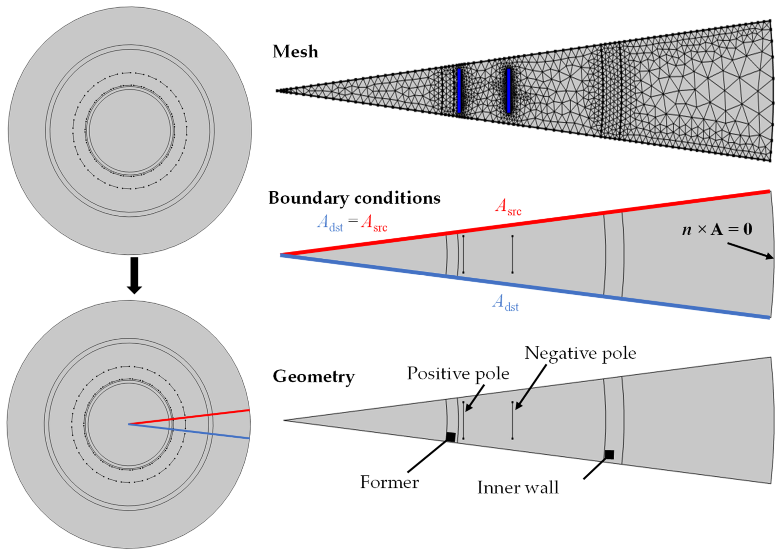
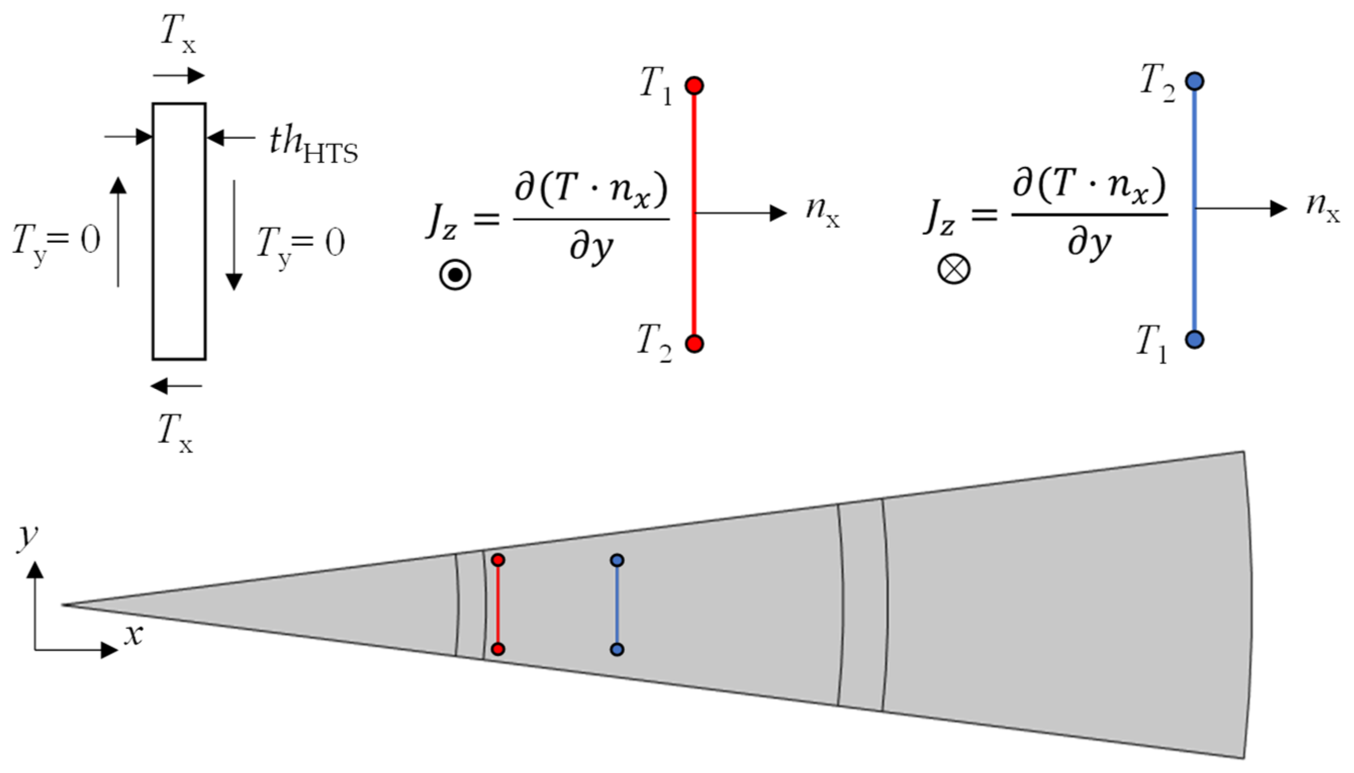
3.4. Modeling of the DC HTS Cable

It is recalled that the superconducting state is limited by three critical quantities. These quantities define a critical surface separating the superconducting state from the normal-resistive state. These three critical quantities are the critical temperature T_c, the critical current density J_c, and the upper critical magnetic field H_c2 for type II superconductors [58,59]. Assuming that the superconductor is well cooled and remains at or close to its operating temperature, two parameters provide a practical limit to the safe and reliable operation of the HTSC, the critical current density and the magnetic field. Both quantities should be evaluated in order to guarantee that the superconductor remains in its superconducting state during operation. The critical current density J_c of the superconductor is inferred from the critical current of the cable I_c as J_c = I_c/A_sc with A_sc as the cross section of the superconductor. The I_c depends on the magnetic field (changing with current) and temperature (here the temperature is assumed to be nearly constant). The upper critical magnetic field H_c2 is essentially given by the chemistry of the material. It is typically replaced by a critical magnetic flux density following B_c = μ₀ H_c2 [60]. These critical quantities are subsequently used in the electromagnetic model of the superconductor in order to define the proper current margin to operate the cable safely and reliably. Undoubtedly, protection and stability features are critical for the application; nevertheless, an appropriate design can enable the operation of the HTSC in the normal-resistive state of the superconductor for a few power cycles in AC or for some time in DC without impairing the stable operation of the power system [61,62].

In order to estimate this margin, it is compulsory to use a model that can include the geometry of the cable in addition to the physics of the superconductor. Indeed, the geometry determines both the magnetic field and the temperature distribution and therefore the impedance of the cable. Such a model can be achieved using the finite element method. As shown in Figure 7, the coaxial cable includes symmetry in the transverse plane. It is therefore possible to simplify the simulation by considering only one single sector of the cable. The opening of the sector is equal to 360°/N, where N is the number of tapes per layer. The periodic condition refers to defining that the magnetic vector potential A is equal on both boundaries of the sector (A_src = A_dst). This simplification reduces the mesh size for the simulation from 165,714 domain elements and 6172 boundary elements without simplification to 5849 domain elements and 422 boundary elements with simplification. Each tape has been discretized into 100 elements corresponding to a 40 µm mesh size.

In addition, by coupling the FE model with an electrical circuit simulating the electrical traction network, it is possible to insert the actual environment and operating conditions seen by the cable. This coupling is then achieved by the estimation of the impedance of the cable from the distributed variables computed by the FE model. The details of the coupling can be found in Section 5.

The FEM implements the T-A formulation of the Maxwell equations, as it is the latest formulation and yields a fair accuracy of the losses at the fastest computation time [63]. This new formulation was cross-checked and validated against the well-established H formulation [64]. The current vector potential T is solved in the superconducting domain Ω_HTS (superconductor layer of each individual tape), whereas the magnetic vector potential A is solved in the complementary domain, which is referred to as the air or A domain Ω_A. The air domain lumps all the surroundings of the superconductor material. The current density J of the superconductor is given by J = ∇ × T.

According to Faraday’s law, the magnetic induction B is related to the electric field E by:

$$\nabla \times E=-\mathsf{\partial }B/\mathsf{\partial }t$$

(6)

The electric field is related to the current density through the resistivity 𝜌 of the superconductor as E = ρ J. The magnetic flux density or magnetic induction B is calculated from A in the air as B = ∇ × A. Replacing the electrical field and the magnetic flux density by their respective potentials lead to two equations relating the magnetic vector potential and the current vector potential. More details on the T-A formulation can be found in [63,65]. In order to impose a transport current in each tape, specific boundary conditions must be added in the T-formulation at the edges of the superconducting tapes, as shown in Figure 8. To account for the direction of the current in the positive and negative poles, it is only required to reverse the position of the conditions at the edges of the tape. The current in an HTS tape can be expressed as follows:

$$I_{\mathrm{T}}=\left(T_1-T_2\right)t{h}_{\mathrm{HTS}}$$

(7)

with T₁ and T₂ being the current vector potentials at the respective edge points.

The electrical resistivity ρ of the superconductor depends on the current density J. This dependence can be expressed near the critical current density J_c by a power law relating the electrical field E along the superconductor to its current density, as follows [34]:

$$\rho =E_{\mathrm{c}}/J_{\mathrm{c}}\cdot {\left(‖J‖/J_{\mathrm{c}}\right)}^{n-1}$$

(8)

where E_c = 1 μV/cm is an arbitrary critical electric field between 1 and 10 μV/cm, and n is the index of transition representing the stiffness at which the voltage increases as the current in the superconductor is increased. In the present study, n is assumed constant and equal to 25 [66]. The most critical point in the cable is given by the maximum temperature which in turn determines the minimum value of the critical current density J_c. Here, we assume that the cable is at the temperature of the liquid nitrogen. Figure 9a illustrates the evolution of the temperature of the liquid nitrogen along the cable length for a “concentric” cooling scheme [67]. This cooling scheme consists of two concentric pipes centered in a single cryostat. The superconducting tapes and the insulation are located between the two pipes. The inner pipe carries the nitrogen from the station to the cable termination and the outer pipe carries the nitrogen back from the termination to the cooling system. The maximum temperature T_LTmax is reached in the outer pipe close to the termination. It should be noted that the shape of the temperature evolution and hence the value of T_LTmax changes according to the cable architecture and the configuration of the cooling system. In the present case, as the same concentric cooling scheme for both cables is employed, T_LTmax is equal to 71.27 K for both the unipolar and bipolar cable topologies.

If J_cB defines the value of the critical current density at T_LTmax in the cable, then J_cB = J_c(T_LTmax, B). Therefore, J_cB depends only on the magnitude and direction of the magnetic flux density B compared to the surface of the tapes, which in turn depend on the radial position of the tape in the cable, thereby explaining the need for computing the distribution of the magnetic flux density in the cable. The J_cB is given by the Kim–Anderson relation so that:

$$J_{\mathrm{cB}}=\frac{J_{\mathrm{c}0}}{{\left(1+\sqrt{k_{\mathrm{a}}{}^2{B}_{//}{}^2+B_{\perp }{}^2}/B_0\right)}^{\beta }}$$

(9)

with k_a = 0.65 being the anisotropy factor, and B₀ = 0.10 T and β = 0.41. J_c0 = 620 A/mm² is the critical engineering current density in self-field at T_LTmax. $B_{//}$ and $B_{\perp }$ are the parallel and orthogonal components of the magnetic flux density B relative to the surface of the tape [68]. Figure 9b depicts the dependence of the critical engineering current density on the direction of the external magnetic flux density for 50 mT and 100 mT at 70 K [69].

The electrical losses Q [W/m] in the superconducting material ${\mathsf{\Omega }}_{\mathrm{HTS}}$ of the HTS cable are computed in the FEM solver as follows:

$$Q(t)={\displaystyle \underset{{\mathsf{\Omega }}_{\mathrm{HTS}}}{\int }E(t)\cdot J(t)\hspace{0.17em}d}{\mathsf{\Omega }}_{\mathrm{HTS}}$$

(10)

The computation of the losses is subsequently used to assess the impact of an HTS DC cable on the global efficiency of the electrical traction network and to compute the equivalent resistance of the superconducting cable.

4. Modeling of an Electrical Traction Network

In this section, the substations and the components of the 1.5 kV traction network are introduced. The network, modeled using lumped parameters, evolves according to the position and power consumption of the trains moving between the substations. The circuit is coupled to an FE model using a co-simulation approach in order to study the impact of an HTS cable on the three main parameters: substation, train, and traction line. These parameters are presented below.

4.1. Modeling of the Substation (SS)

In the field of railway electrification, SS are the sources of electrical power supplied to the traction lines. In France, 1.5 kV SS are generally connected to a three-phase high voltage (HV) grid with rated voltages equal to 63 kV or 90 kV at a frequency of 50 Hz in order to comply with the French Electricity Transmission Network (Réseau de transport d’Electricité or RTE) and a rated voltage of 20 kV for a connection to the Electricity of France (Electricité De France or EDF). Figure 10a shows an example of a connection to the EDF grid. For redundancy, two step-down transformers and two rectifiers connect the HV grid to the low-voltage DC output. The substations are also linked to two independent HV grids, which guarantees continuity of service during incidents or maintenance. On the EDF side, the primary windings of the transformers are supplied by a 20-kV line-to-ground voltage. Generally, the power of the substation is achieved by two step-down transformers in parallel, coupled to a rectifier system in series or in parallel. Typical substation ratings are 4.4 MW, 6.6 MW, and 10 MW, depending on the loads (passenger train, freight train, etc.). In addition, a twelve-pulse transformer is often chosen to suppress harmonics up to rank 11. The rectifier shown in Figure 10 is a double Graetz bridge with diodes at a rated power of 6.6 MW for 1.5 kV and a DC nominal current of 4.4 kA. Depending on the substation, a DC circuit breaker is installed between the rectifier and the line. It has a rated current between 4 kA and 6 kA, a breaking capacity of up to 60 kA, and a tripping time of a few tens of milliseconds.

Figure 10b shows the equivalent circuit of the substation implemented in Simulink. A self-inductance L_SS located at the output of the substation is introduced in order to smoothen the current variation (di/dt) due to the transients induced by the train accelerations and deaccelerations.

4.2. Modeling of the Train

The modeling of the train is based on the determination of its mechanical power, P_m, which can be expressed as the product of the torque C_m and the angular velocity ω_m:

$$P_{\mathrm{m}}=C_{\mathrm{m}}{\omega }_{\mathrm{m}}(1+\mathrm{sgn}(C_{\mathrm{m}})(1-n_{\mathrm{v}}\left)\right)$$

(11)

with n_v being the efficiency of the gearbox. The sign function sgn(C_m) of the torque is equal to +1 when the train is operated in motor mode and −1 in braking mode. As the trains are equipped with purely mechanical brakes, there is no energy recovery. An equitable distribution of the torque is assumed over all the n_w cars, i.e., all of the cars have the same torque per axle. The number of axles per car is n_r. Therefore, the torque per axle is expressed as C_m = r F_TF/(n_wn_r) and the angular velocity per axle is given by ω_m = v/r with r being the wheel radius. The tractive force F_TF necessary to ensure the movement of a train is given by the Newton’s second law of motion, yielding

$$P_{\mathrm{m}}=C_{\mathrm{m}}{\omega }_{\mathrm{m}}(1+\mathrm{sgn}(C_{\mathrm{m}})(1-n_{\mathrm{v}}\left)\right)$$

(12)

$$F_{\mathrm{grd}}=m_{\mathrm{t}}g\cdot \sin (\alpha )$$

(13)

$$F_{\mathrm{rol}}=m_{\mathrm{t}}g\cdot F_{\mathrm{r}0}\cdot \cos (\alpha )$$

(14)

$$F_{\mathrm{dyn}}=0.5 {\rho }_a\cdot S_{\mathrm{T}}\cdot C_{\mathrm{T}}\cdot v^2$$

(15)

Figure 11 illustrates the different forces. F_rol is the rolling resistance force, F_dyn is the aerodynamic drag force, and F_grd is the gradient force due to the slope or inclination of the train track. ρ_a is the air density in kg/m³, v is the train speed in m/s, S_T is the train frontal area, and g = 9.81 m/s² is the standard value of the earth gravitational acceleration. C_T and F_r0 are the aerodynamic drag coefficient and the rolling resistance coefficient, respectively. m_t is the total mass of a train and $\alpha$ is the angle of inclination.

From these expressions, the inrush currents I_Tk of the train k, with k = {1, 2}, can be written as a function of the electrical power of the train and the voltage available at their current positions between the substations:

$$I_{\mathrm{Tk}}(t)=n_{\mathrm{w}}\cdot n_{\mathrm{r}}\cdot n_{\mathrm{m}}\cdot n_{\mathrm{i}}\frac{P_{\mathrm{mk}}(t)}{V_{\mathrm{Tk}}(t)}+n_{\mathrm{w}}\frac{P_{\mathrm{ak}}(t)}{V_{\mathrm{Tk}}(t)}$$

(16)

P_mk is the electrical power needed to ensure the movement of the train, and P_ak is the electrical power needed for the auxiliary systems, such as lighting, air conditioning, etc. The power of the auxiliaries can be degraded or deactivated when the power limit of the SS is reached. In the present simulation, P_ak was kept constant and equal to 50 kW per car, which corresponds to a maximum continuous operation of the auxiliaries for the train category under study.

4.3. Modeling of the Traction Line

Figure 12 illustrates the circuit of the traction line indicating the train position p_Tk(t). p_Tk was found between the position of substation 1 (p_SS1) and the position of substation 2 (p_SS2). The impedances of the traction line were calculated at each time step based on the train position. Their expressions are summarized in

Table 2. Expression of the different linear impedances Z (Ω/km) as a function of train position p_Tk.

	Position	$p_{\mathrm{Tk}}(t)\le p_{\mathrm{HTS}}$	$p_{\mathrm{Tk}}(t)>p_{\mathrm{HTS}}$
Zl1(t)	Bipolar HTSC	$Z_{\mathrm{l}}{p}_{\mathrm{Tk}}(t)$	$Z_{\mathrm{l}}(p_{\mathrm{SS}1}-p_{\mathrm{HTS}})$
	Unipolar HTSC	$Z_{\mathrm{l}}{p}_{\mathrm{Tk}}(t)$	$Z_{\mathrm{l}}(p_{\mathrm{SS}1}-p_{\mathrm{HTS}})$
Zl2(t)	Bipolar HTSC	$Z_{\mathrm{l}}((p_{\mathrm{SS}1}-p_{\mathrm{HTS}})-p_{\mathrm{TK}}(t))$	0
	Unipolar HTSC	$Z_{\mathrm{l}}((p_{\mathrm{SS}1}-p_{\mathrm{HTS}})-p_{\mathrm{TK}}(t))$	0
Zl3(t)	Bipolar HTSC	0	$Z_{\mathrm{l}}(p_{\mathrm{TK}}(t)-(p_{\mathrm{SS}1}-p_{\mathrm{HTS}}))$
	Unipolar HTSC	0	$Z_{\mathrm{l}}(p_{\mathrm{TK}}(t)-(p_{\mathrm{SS}1}-p_{\mathrm{HTS}}))$
Zl4(t)	Bipolar HTSC	$Z_{\mathrm{l}}((p_{\mathrm{SS}2}-p_{\mathrm{SS}1})-(p_{\mathrm{SS}1}-p_{\mathrm{HTS}}))$	$Z_{\mathrm{l}}((p_{\mathrm{SS}2}-p_{\mathrm{SS}1})-(p_{\mathrm{SS}1}-p_{\mathrm{HTS}})-P_{\mathrm{Tk}}(t))$
	Unipolar HTSC	$Z_{\mathrm{l}}((p_{\mathrm{SS}2}-p_{\mathrm{SS}1})-(p_{\mathrm{SS}1}-p_{\mathrm{HTS}}))$	$Z_{\mathrm{l}}((p_{\mathrm{SS}2}-p_{\mathrm{SS}1})-(p_{\mathrm{SS}1}-p_{\mathrm{HTS}})-P_{\mathrm{Tk}}(t))$
Zr1(t)	Bipolar HTSC	$Z_{\mathrm{r}}{p}_{\mathrm{Tk}}(t)$	$Z_{\mathrm{r}}(p_{\mathrm{SS}1}-p_{\mathrm{HTS}})$
	Unipolar HTSC	$Z_{\mathrm{r}}{p}_{\mathrm{Tk}}(t)$
Zr2(t)	Bipolar HTSC	$Z_{\mathrm{r}}((p_{\mathrm{SS}1}-p_{\mathrm{HTS}})-p_{\mathrm{TK}}(t))$	0
	Unipolar HTSC	$Z_{\mathrm{r}}((p_{\mathrm{SS}1}-p_{\mathrm{HTS}})-p_{\mathrm{TK}}(t))$
Zr3(t)	Bipolar HTSC	0	$Z_{\mathrm{r}}(p_{\mathrm{TK}}(t)-(p_{\mathrm{SS}1}-p_{\mathrm{HTS}}))$
	Unipolar HTSC	NA	NA
Zr4(t)	Bipolar HTSC	$Z_{\mathrm{r}}((p_{\mathrm{SS}2}-p_{\mathrm{SS}1})-(p_{\mathrm{SS}1}-p_{\mathrm{HTS}}))$	$Z_{\mathrm{r}}((p_{\mathrm{SS}2}-p_{\mathrm{SS}1})-(p_{\mathrm{SS}1}-p_{\mathrm{HTS}})-P_{\mathrm{Tk}}(t))$
	Unipolar HTSC	NA	NA

. Z_l and Z_r represent the impedances of the line and the rail, respectively. The resistance of the line is 28 mΩ/km, and that of the traction rails is 16 mΩ/km. Their inductances are equal to 0.8 and 0.7 µH/km, respectively. The movement of the train on the traction line requires solving two electrical circuits. The first circuit solves the train’s position between SS1 and the superconducting cable injection point p_HTS, p_Tk(t) ∈ [p_SS1, p_HTS]. The second circuit corresponds to a train position between p_HTS and p_SS2.

For the bipolar cable model depicted in Figure 12a, a switch is installed upstream and downstream from the train to prescribe the two possible scenarios when the train moves from SS1 to SS2. Figure 12b shows the unipolar case where a single switch is placed at the overhead traction line, since the cable carries the current from the substation to the injection point and its return is provided by the rails. Figure 12c shows the case where the train is located between SS1 and the injection point of the HTSC, p_HTS. Here, switch P1 is closed and switch P2 is open. As soon as the train passes the HTSC injection point, the states of P1 and P2 are swapped, as shown in Figure 12c,d.

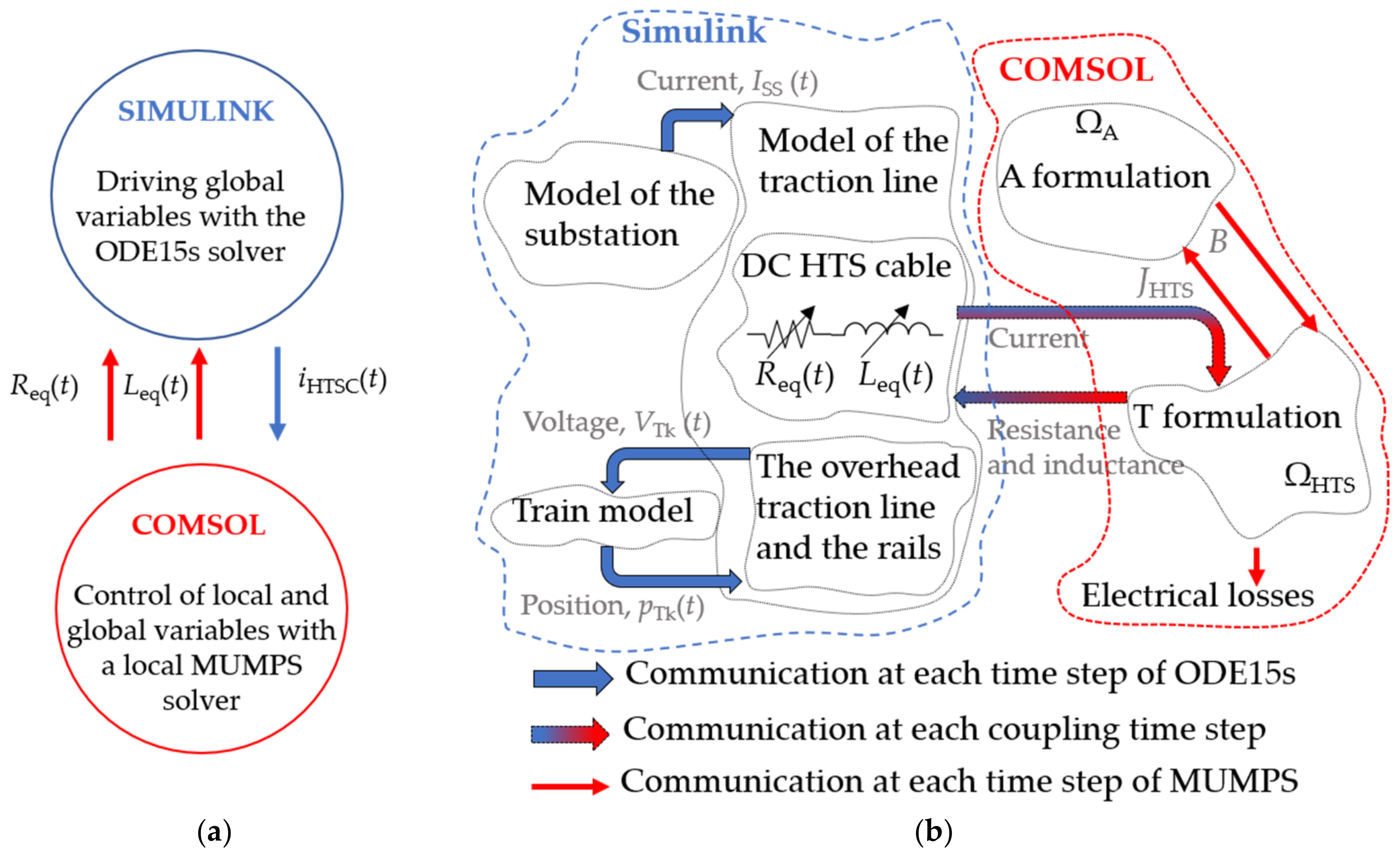
5. Co-Simulation: FEM (Cable) and Circuit (Traction Network)

The coupling is carried out by the Simulink LiveLink^TM toolbox of the FEM software COMSOL 5.6. The layout of the co-simulation is shown in Figure 13a,b. Figure 13a shows the exchange of variables between Simulink and COMSOL. Simulink processes the global variables such as voltage and current, whereas COMSOL treats the distributed variables such as current density and magnetic field. In the present case, the communication time step between the software is fixed by the user at 0.1 ms.

From a purely electric point of view, as shown in Figure 13b, the cable can be represented by an equivalent resistance R_eq(t) and an equivalent inductance L_eq(t) which are computed in Simulink. The resistance of the cable R_eq is determined from the ratio between the electrical losses Q and the square of the current I_HTSC supplied to the HTSC. The value of L_eq is obtained from the magnetic energy W_m computed in COMSOL as follows:

$$R_{\mathrm{eq}}(t)=Q(t)/I_{\mathrm{HTSC}}{}^2(t)$$

(17)

$$L_{\mathrm{eq}}(t)=2W_{\mathrm{m}}(t)/I_{\mathrm{HTSC}}{}^2(t)={\displaystyle \underset{{\mathsf{\Omega }}_{\mathrm{HTS}}}{\int }A(t)\cdot J(t)d{\mathsf{\Omega }}_{\mathrm{HTS}}}/I_{\mathrm{HTSC}}{}^2(t)$$

(18)

where A is the magnetic vector potential computed in the whole domain including the HTSC and its surrounding, and J is the current density of the superconductor.

6. Results and Discussion with Constant Speed Trains

In this section, we will study the impact of the superconducting cable on the railway network for a constant dynamic behavior (at constant speed). We consider three different study cases:

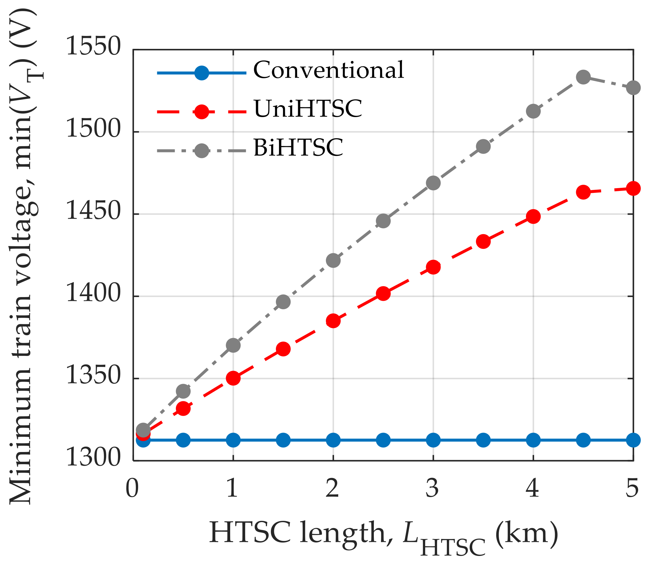
• A railway network without a superconducting cable (referred to as “conventional”);
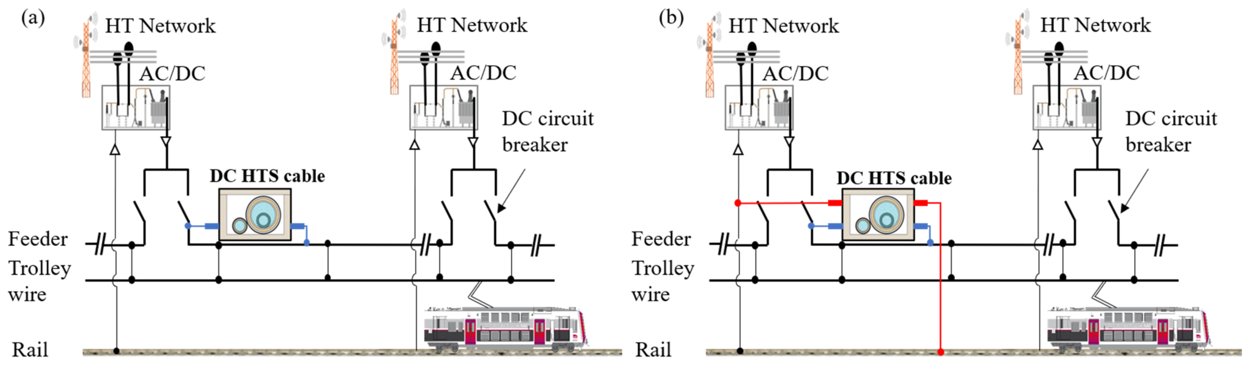
• A railway network with a unipolar superconducting cable (referred to as “UniHTSC”). The cable connects the substation 1 to the injection point p_HTS of the overhead line and the return of the current through the rails;
• A railway network with a bipolar superconducting cable (referred to as “BiHTSC”). The cable connects substation 1 to the overhead traction line at p_HTS and the return of the current to substation 1 is also guaranteed by the same cable.

The traction network parameters are identical for all cases. The model contains two identical substations of 6.6 MW that can provide up to 10 MW of peak power with a no-load voltage of 1750 V. The distance between the two substations is 10 km, i.e., pSS1 = 0 m and pSS2 = 10 km.

The train model is Z 20900, which belongs to the family Z 2N of the French national railroads (SNCF). Their parameters are summarized in

Table 3. Electric and geometric parameters of the trains.

Parameter	Unit	Value
Rated voltage	kV	1.5
Rated power	MW	3.464
Traction force	kN	310
Mass	T	245
Length	M	103.508
Width	M	2.280
Height	M	4.320
Capacity	Passengers	1598
Maximum speed	km/h	140

. Such trains can reach a maximum speed of 140 km/h. For these models, two types of power supplies are used either for feeding the train with a direct current at 1.5 kV or with an alternating current at 25 kV/50 Hz. In the present study, the DC rated power of the trains is given as equal to 3.464 MW. The tractive force is 310 kN with a mass of 245 t without passengers. The length of the trains is 103.50 m, and the size of the frontal area is 2.82 m × 4.32 m. Even though their maximum speed is 140 km/h, the studies, typically carried out by SNCF, consider a steady-state regime at 60 km/h. This speed is used in the present study. The trains are operated at their peak load in order to simulate the most critical case. Hence, the total mass of trains is given by mt = 245 [t] + 0.075 [t] × 1598, where the number 1598 is the maximum number of passengers that the train can carry, and 0.075 [t] is the average mass per passenger.

In this study, the cable lengths range from 0.1 km to 5 km (i.e., 0.1 km < L < (p_SS1 − p_SS2)/2). As mentioned earlier, the sizing method and the necessary tools used are detailed in [67]. The electrical parameters of all cables are identical and are presented in

Table 4. Electrical parameters used for cable sizing.

Parameter	Unit	Value
Nominal voltage\at no load	kV	1.5\1.75
Nominal\Maximum current	kA	4.4\6.75
Nominal\Maximum power	MW	6.6\10.125
Number of layers per pole 1	--	1 or 2
Critical current at 70 K\78 K	A	285\210
Number of tapes per layer	--	UniHTSC	Pole (+)	27
		BiHTSC	Pole (+)	27
			Pole (−)	28

¹ A 1 is given for diameters of the former greater than or equal to 40 mm, 2 for diameters of the former less or equal to 32 mm.

. During normal operation, the cable can withstand 4.4 kA at 1500 V; it can withstand up to 6.75 kA in overload mode. The number of layers per pole for UniHTSC and BiHTSC cases can vary depending on the dimensions of the former of the cable, as shown in Table 4, for diameters of 25 mm and 32 mm the cable contains two layers per pole. On the other hand, for diameters greater than or equal to 40 mm, all of the tapes are arranged on a single layer.

In

Table 5. Thermal and hydraulic parameters used for cable sizing.

Parameter	Unit	Value
Input temperature (LN2)	K	68
Initial pressure (LN2)	bar	15
Output temperature (LN2) 1	K	<78
Mass flow rate	kg/s	[0.1; 2]
Pressure drop1	bar	<10

¹ Indicates that the value may change depending on the length of the cable, but it is always lower than the indicated value.

, the hydraulic and thermal parameters of the cable are indicated. The initial operating temperature is 68 K with a pressure of 15 bar. Depending on the length of the cable, the liquid nitrogen flow rate can vary between 0.1 kg/s and 2 kg/s. For short cables, a low flow rate allows the cable to be cooled while respecting the thermal and hydraulic constraints. For long cables, however, a higher nitrogen flow rate is required to cool the cable. The selection of the flow rate must ensure that the maximum temperature of the liquid nitrogen in the cable is always below 78 K and that the pressure drop is always below 10 bars.

6.1. Influence of the Insertion of a HTSC on the Voltage Drop of Traction Lines

In this section, the impact of the HTSC on the reduction of the voltage drop along the traction line is estimated. For this case study, the length of the superconducting cable is kept constant and equal to 1.5 km.

Figure 14a shows the train voltage as a function of its position for the three cable technologies. The train speed is equal to 60 km/h, and the total electrical power of the trains is equal to 4.9 MW. The voltage drop on the traction lines is lower with an HTSC than with a conventional cable, as demonstrated by the minimum voltage value min(V_T) equal to 1312 V for the conventional cable, and 1367 V, and 1396 V for the UniHTSC and BiHTSC, respectively. At the cable injection point p_T = p_HTSC = 1.5 km, significant reductions are observed with 108 V and 171 V for the unipolar and bipolar cases, respectively. The difference between the UniHTSC and the BiHTSC is due to the flow of the return current to the SS, which passes through the HTSC in the BiHTSC case and not through the resistive rail for UniHTSC.

Figure 14b shows the influence of the train power on the minimum voltage available on the network. As the train power increases, the minimum voltage decreases. Indeed, an increase in power requires more current, so the line losses rise, thereby generating a greater voltage drop. Interestingly, with a higher power, the two topologies, UniHTSC and BiHTSC, have a more significant impact on the reduction of the voltage drop. Thus, for a power of 1.4 MW, the voltage drop reduction is about 10 V and 15 V for UniHTSC and BiHTSC, respectively, while the reduction is about 79 V and 118 V for a power of 5.6 MW.

From these results, it can be inferred that the superconducting cables for both topologies can effectively reduce the voltage drop along the traction lines. The BiHTSC appears as the best option to reduce the voltage drop for a given cable length and train power.

6.2. Influence of the Length of the HTSC on the Voltage Drop of the Traction Lines

In this section, the impact of the cable length on the voltage drop reduction is estimated. The distance between the two substations is 10 km, and the electrical power of the trains is kept at a constant power equal to 4.2 MW. Figure 15 shows the minimum train voltage, min (VT), as a function of the length of the superconducting cable. With a longer cable length, a reduction of the voltage drop along the traction line can be observed. Thus, for a 1 km HTSC cable, the minimum train voltage is equal to 1350 V and 1370 V for the UniHTSC and BiHTSC cases, while it is equal to 1466 V and 1527 V for a 5 km-long cable.

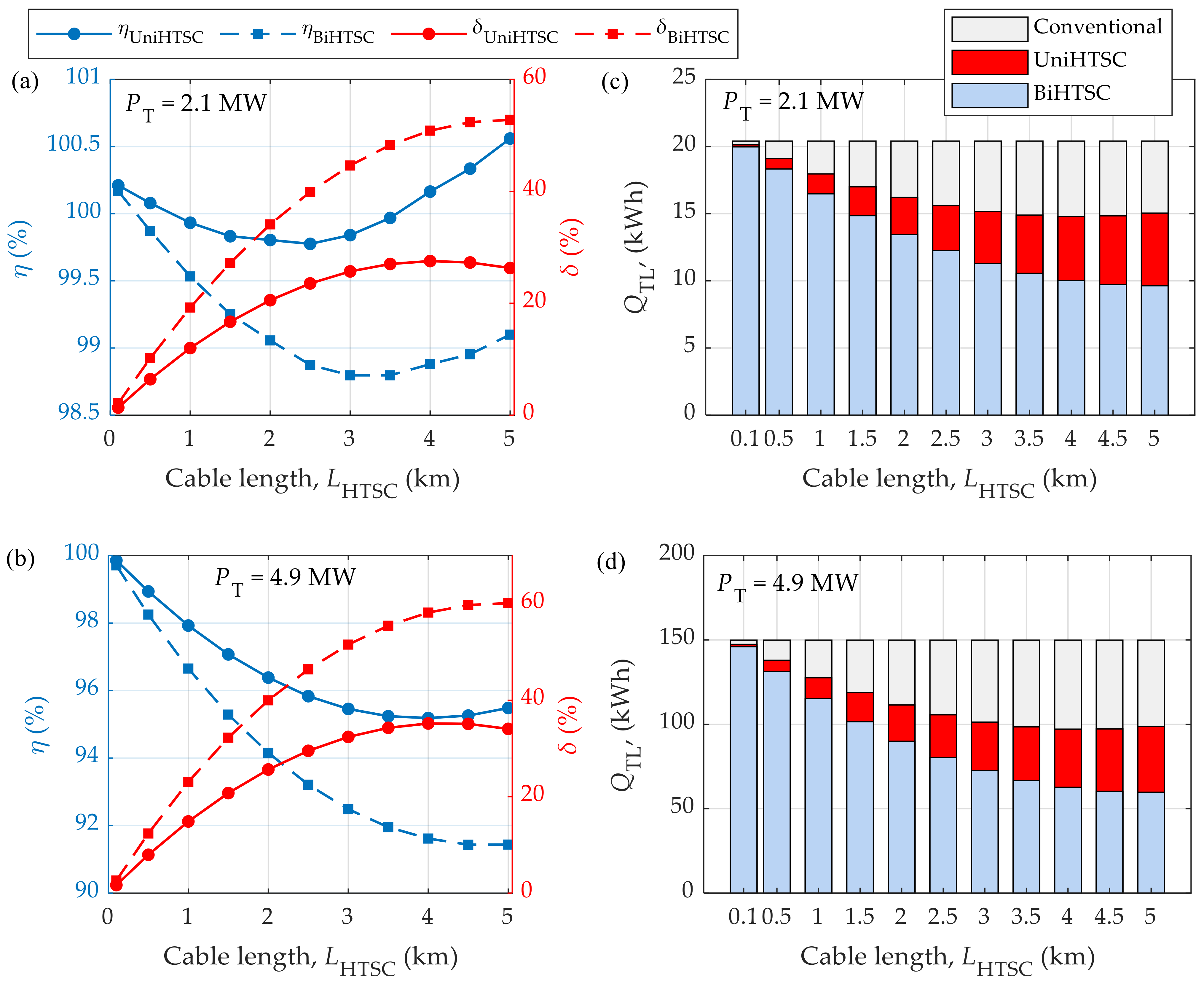
6.3. Influence of HTSC Length on Energy Consumption

In this section, the ratio of the energy consumed by the whole system for the superconducting cables over the energy consumption of the whole system for the conventional cable in percent η and the relative energy consumption of the traction line (TL) in percent δ are presented for the three cable technologies: conventional, UniHTSC, and BiHTSC. δ is an indication of the electrical impact of the superconducting cable on the traction line. The whole system is defined as the traction line in the case of the conventional cable and the traction line adding the superconducting cable, its terminations, and cooling system for the UniHTSC and BiHTSC cases. The mathematical expressions of the ratio η and the relative TL consumption δ are as follows:

$$\eta /100=\frac{Q_{\mathrm{HTSC}}}{Q_{\mathrm{Conv}}}$$

(19)

$$\delta /100=(Q_{\mathrm{TL},\mathrm{Conv},}-Q_{\mathrm{TL},\mathrm{HTSC}})/Q_{\mathrm{TL},\mathrm{Conv}}$$

(20)

where Q represents the total energy of the system; Q_Conv = Q_SS1,Conv + Q_SS2,Conv for the conventional cable and Q_HTS = Q_SS1,HTSC + Q_SS2,HTSC + Q_cooling for the superconducting cables. Q_SS1 and Q_SS2 depend on the traction line efficiency. Therefore, as the superconducting cable inherently dissipates less than the conventional cable, Q_SS1,HTSC + Q_SS2,HTSC < Q_SS1,Conv + Q_SS2,Conv in any normal operating conditions. Q_TL represents the energy consumed by the traction line through its circuit impedance. It is defined as follows:

$$Q_{\mathrm{TL}}=\hspace{0.33em}{\displaystyle \sum _i{\displaystyle {\int }_0^t{Z}_i{I}_i^{2}dt}}$$

(21)

where i is the index of an electrical branch in the traction line, Z_i is the impedance of the branch i and I_i is its current.

Figure 16 shows the evolution of the parameters δ and η and the energy Q_TL as a function of the superconducting cable length for two magnitudes of train electrical power, 2.1 MW and 4.9 MW. Figure 16a shows an increase in δ for both UniHTSC and BiHTSC cases, indicating that less energy is needed to supply the traction line; in other words, there is less dissipation than in the conventional case. The superconducting cable is inherently less resistive than a conventional cable. Nevertheless, it should be noted that, in the present case, the power demanded by the cooling system should also be added to the total electrical power. This power is included in the ratio η. In some cases, there are configurations for which the installation of a superconducting cable is not beneficial in terms of reducing the overall energy consumption. Indeed, the voltage drop reduction alone is not a decisive factor for the choice of the technology, as the energy budget impacting the cost of operation should be included as well. For instance, a UniHTSC having a length of 0.5 km or a length greater than 3.5 km requires more energy as a whole than a conventional cable. In those cases, Q_cooling tips the energy supplied by the SS leading to η > 100%. For cable lengths between 1 km and 3 km, η is inferior to 0.3% indicating that the gain in the overall energy consumption is miscellaneous, and there is no significant impact of the superconducting technology in terms of energy gain compared to a conventional cable. Nevertheless, it still provides a reduction in the voltage drop. In the BiHTSC case, the HTSC conveys a larger improvement on the total system consumption for any cable length, making it the most promising technological solution. For both UniHTSC and BiHTSC topologies, η tends to decrease as the energy needed to maintain the HTSC at nominal temperature increases at a lesser rate than the electrical energy needed to supply a conventional cable.

Figure 16b shows that for P_T = 4.9 MW, the reduction of the energy consumed by the traction line and the energy consumed by the complete system are always ensured with a superconducting cable. As the length of the cable is increased, the total energy consumption decreases. In the case of the BiHTSC, a reduction of 3.3% and 8.6% is achieved for a length of 1 km and 5 km, respectively.

There are clear benefits to using superconducting cable, as has been shown previously. The technology, particularly in its bipolar topology, could allow more trains to circulate on the track with the same installation or increase the life cycle of the traction line. In any case, the total energy budget including the cooling system should be assessed, as the total amount of electrical energy needed to operate the trains using a superconducting cable may be larger than that using conventional technology. This larger electrical energy consumption translates into additional operating costs. On the positive side, the gain in energy consumption brought by a superconducting cable becomes greater and greater as the power of the trains increases. For railway facilities where the number of running trains has increased significantly over the past years, the installation of superconducting cables can increase the service life of the original infrastructure without the necessity of electrical and civil changes to accommodate the growth in power demand.

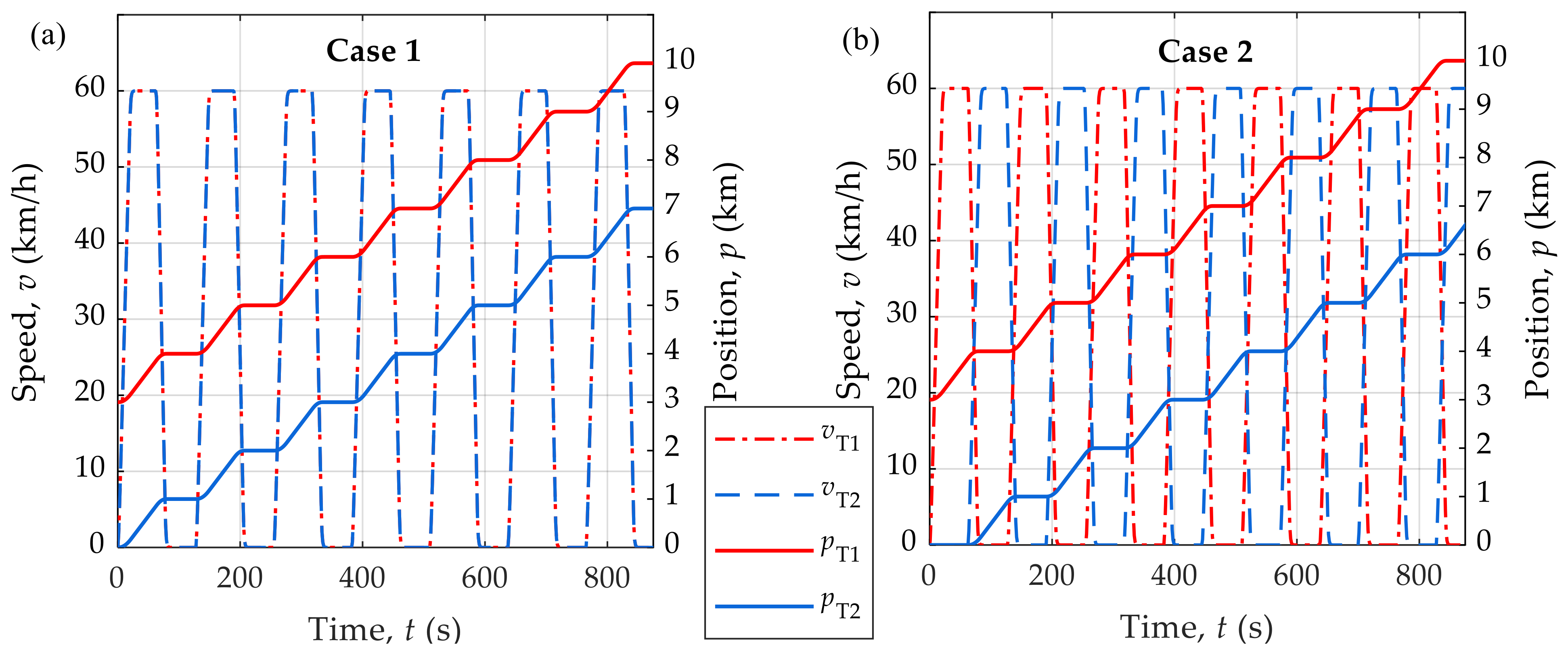
7. Results and Discussion with Variable Speed Trains

In the previous section, it was shown that the reduction of the energy consumed by the traction line depends mainly on the power of the trains. In order to estimate this reduction, it is necessary to consider the geometrical and electrical characteristics of the superconducting cable as well as the phenomenon of the superconductivity, multiphysics in nature. These characteristics change dynamically if external conditions evolve. Hence, as the trains accelerate and deaccelerate/brake between substations, it is essential to include a detailed transient analysis of the electrical behavior of the railway network to design the superconducting cable with its cryogenic system and to assess properly its behavior and impact.

The impact of the cable on the main elements of a railway network during travel between two substations is subsequently assessed. These main components are the substations, the trains, and the traction lines.

Two scenarios, presented in Figure 17, are considered:

• Both trains have the same dynamic behavior at their respective positions, Figure 17a;
• Both trains have an identical speed profile, but these profiles are delayed by about one minute, as shown in Figure 17b.

These scenarios represent speed profiles that are typically found in the operation of actual trains on the French traction network. In the present case, the speed profiles are as follows: the trains have an acceleration of 3 km/h/s for 20 s, followed by a constant velocity of 60 km/h for 40 s, a deceleration of 5 km/h/s for 15 s, and a pause at the train station lasting 45 s. These are the limits imposed by the railway company on the train driver at SNCF.

The unipolar and bipolar superconducting cables have the same length of 1.5 km.

Table 6. Parameters of the unipolar and bipolar superconducting cables.

Parameter	Unit	UniHTSC	BiHTSC
Number of layers per pole	--	1	1
Standard former (inside\outside)	mm	40 (40\42.8)	40 (40\42.8)
Diameter of the superconducting layers	mm	42.8\43.1	Pole (+)	42.8\43.1
			Pole (−)	49.1\51.1
Insulating layer between the poles	mm	NA	6
Number of tapes per layer	--	27	Pole (+)	27
			Pole (−)	28
Minimum critical current at 72 K	A	251	248
Standard diameter of inner pipe (inside\outside)	mm	100 (79.8\83.8)	120 (99.8\104.4)
Standard diameter of outer pipe (inside\outside)	mm	120 (125.6\130.8)	150 (151.9\157.9)
Length	km	1.5
Mass flow rate	kg/s	0.5	0.6
Pressure drop	bar	3.2	4.5
Maximum temperature	K	72.5

shows the different parameters of the cables. Their nominal current is about 4.4 kA, and their critical current is I_c ≈ 1.5 × I_n = 6.75 kA. The liquid nitrogen inlet temperature is 68 K and the temperature difference between the inlet and the outlet is less than 4 K for the UniHTSC and the BiHTSC, see Figure 9a. The pump flow rate is 0.5 kg/s with a pressure drop below 4 bar for cryostat losses of 1.5 W/m. Figure 17 shows the positions of the two identical trains T1 and T2 between SS1 and SS2. The path between SS1 and SS2 contains 11 train stations separated by a distance of 1 km (blue circles in Figure 17c). At t = 0 s, T1 is located at p_T1 = 0 and T2 is located at p_T2 = 3 km. T1 is upstream from the superconducting cable injection point p_HTS, and T2 is downstream from p_HTS, so that T1 and T2 are 1.5 km away from the superconducting cable injection point p_HTS.

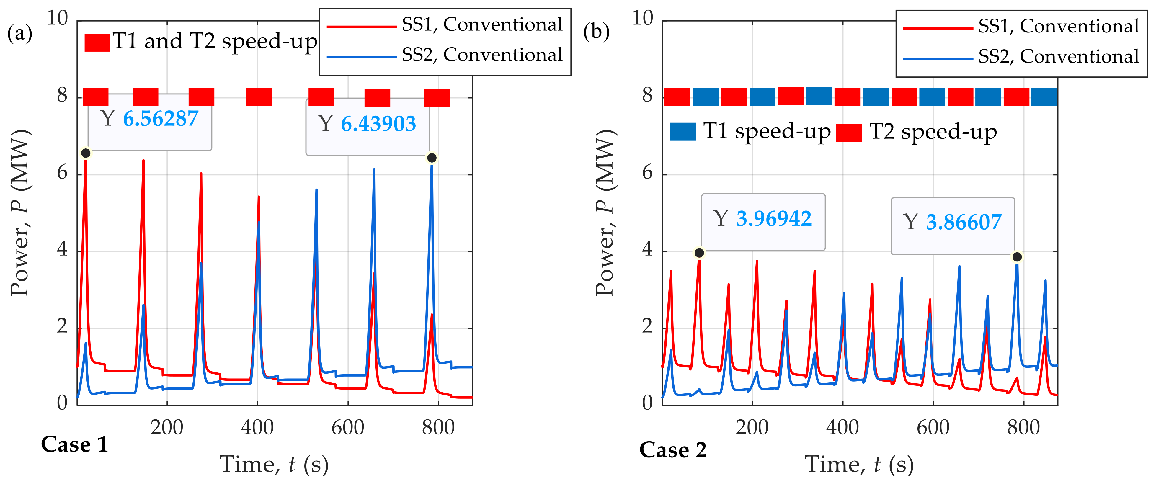
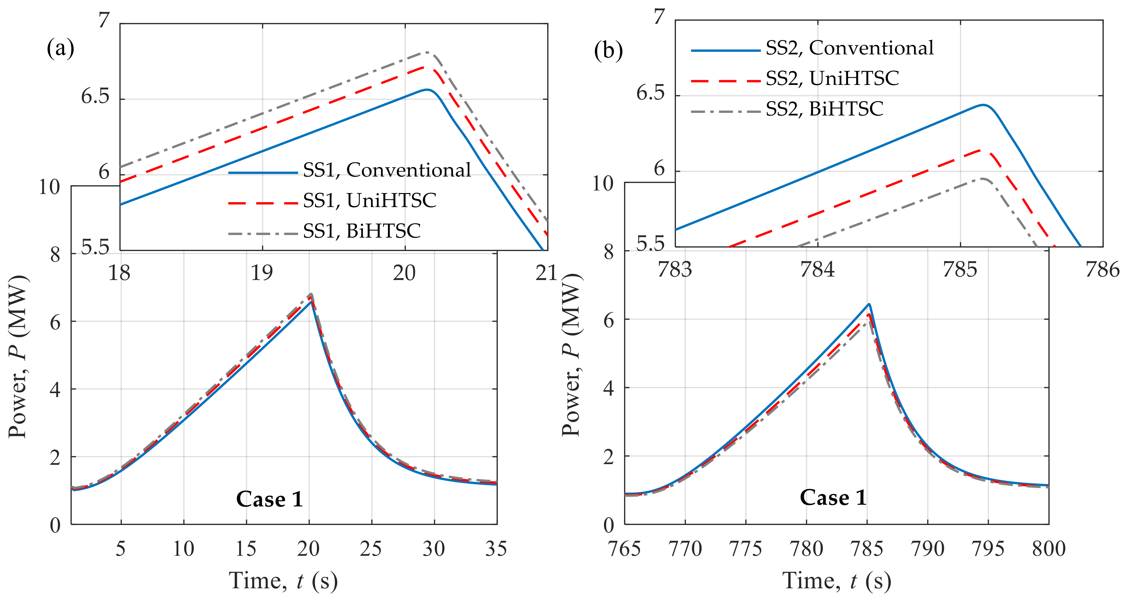
7.1. Influence of HTSC on the Substations

Figure 18 shows the instantaneous power supplied by the substations for the conventional case (no HTSC) and the two mentioned speed profiles, scenarios 1 and 2. Figure 18a shows scenario 1, while Figure 18b shows scenario 2. For both scenarios, the impedances between the substations and the trains depend on the location of the trains. For the following, two trains are leaving the same station SS1. As they leave SS1, the impedances between the trains and SS1 are lesser than the impedances between the trains and SS2. Consequently, more current and more power is drawn from SS1. However, as the trains are getting away from SS1 and therefore getting closer to SS2, more power is drawn from SS2. For scenario 1, more power (6.56 MW for SS1 and 6.44 MW for SS2) is supplied by the substations, since both trains are moving at the same time following the same speed profile. However, in scenario 2, when one train is moving, the other is at rest. Consequently, both substations supply less than 4 MW at peak.

The total consumption of the complete system is equal to 487 kWh, 479 kWh, and 475 kWh for the conventional, UniHTSC, and BiHTSC cases, respectively. This represents a reduction in the total electrical consumption of 1.6% and 2.5% brought by the superconducting cables compared to the conventional one.

Figure 19a shows the peak of the evolution over time of the instantaneous power supplied by SS1 to all cable technologies when the trains are close to SS1. The peak of instantaneous power for the conventional cable is 6.56 MW, while it is 6.7 MW and 6.91 MW for UniHTSC and BiHTSC, respectively. Similarly, Figure 19b shows the peak of instantaneous power supplied by SS2 for all the cables when the trains are close to SS2. The peak of instantaneous power for the conventional cable is 6.43 MW, while it is 6.20 MW and 6.05 MW for the UniHTSC and the BiHTSC, respectively. Thus, by adding a HTSC close to SS1, the equivalent impedance between the HTSC and the overhead line (including the rails for scenario 2) diminishes. Compared to the conventional cable, more power is then drawn from SS1. Conceptually, the distances between the trains and SS1 have been shortened.

The location of the HTSC may be further optimized, as it plays a significant role in the power management of the traction network. It should be noted that the basic feature of the HTSC for both topologies is the mitigation of the increase in the voltage drop along the line due to aging equipment and/or an increase in the number of trains on the track as shown in the previous sections.

7.2. Influence of HTSC on the Traction Line

Figure 20 shows the electric energy consumption of the traction lines for the total current equal to 4.4 kA. The consumption in scenario 1 is higher than in scenario 2, 34.32 kWh against 25.30 kWh. This increase arises from the simultaneous acceleration of both trains, which requires a higher operating current. Figure 20a shows the energy consumption of the three cable technologies for scenario 1. For this scenario, the insertion of the superconducting cable on the line strongly reduces the consumption of the traction line and consequently lowers the Joule losses. The reduction in energy consumption is 21.3% with the UniHTSC and 33.7% with the BiHTSC.

Concerning the overhead line losses, a slight difference between the UniHTSC and the BiHTSC can be observed, with energies of 15.05 kWh and 14.54 kWh, respectively. This difference results from the difference in magnitude of the transmission currents between the two topologies for the same mechanical traction power. The UniHTSC requires more current than the BiHTSC, as the latter generates less voltage drop than the former.

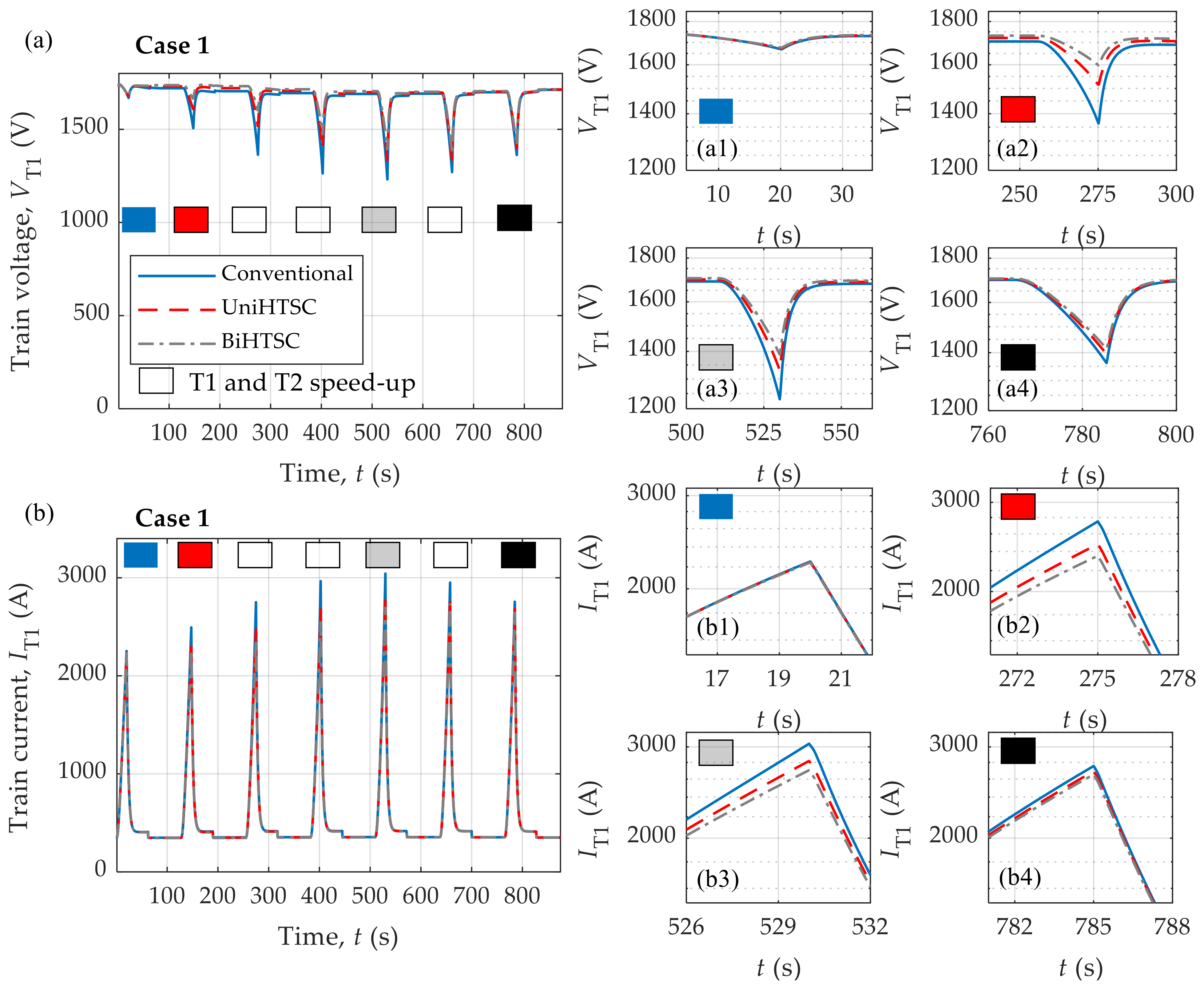
7.3. Influence of HTSC on the Trains

Figure 21 shows the voltage V_T1 and the current I_T1 absorbed by train T1 for the three cable technologies in scenario 1. At t = 0 s, T1 is located upstream from the injection point p_HTS. It can be observed that the insertion of the superconducting cable decreases the voltage drop at the train for lesser current consumption. For instance, at t = 275 s, V_T1 is equal to 1364 V for the conventional cable and equal to 1486 V and 1545 V for UniHTSC and BiHTSC, respectively. It is recalled that BiHTSC provides a return path for the current avoiding the resistive rails, which allows for further lowering of the voltage drop. The minimum voltage of train T1 is equal to 1297 V for scenario 1. In this condition, both trains accelerate at the same time which generates a larger peak of current than the one found in scenario 2 for which there is a 1 min delay between the train departure. Furthermore, Figure 21(a1–a4) shows that the train voltage V_T1 is sustained by the HTSC when the train is close to the injection point of the superconducting cable. Conversely, if T1 is farther away from the injection point, then the influence of the cable presence on the train voltage decreases, as depicted by Figure 21(a4), and the voltage drop deepens. Indeed, from t < 450 s, it is SS2 that feeds T1 and not SS1 where the cable is connected, as illustrated by Figure 17a.

Figure 21b shows the current consumption of train T1 for the three cables in scenario 1. Following the reduction of the voltage drop with the insertion of the superconducting cable, a reduction of the current consumed by the train is also achieved for the same mechanical power. For instance, at t = 275 s, the reduction in the train current is about 7.9% and 11.9% for the UniHTSC and the BiHTSC, respectively.

It can be concluded that the insertion of a superconducting cable in the DC railway network can effectively lower the voltage drop along the traction line. In particular, the reduction of the current absorbed by the train for the same mechanical power lowers the dynamic losses, thereby increasing the overall efficiency. Consequently, a larger margin of power drawn by the trains is achieved, increasing the life cycle of the installation, as less current is required for the same or more traffic (more passengers per journey).

7.4. Electrical Losses in HTSC

The amount of electrical losses generated in the HTSC is calculated and shown in Figure 22. The second y-axis, on the right side of the figures, presents the ratio between the transport current and the critical current of cable I/I_c. This fraction represents the current margin of the superconducting cable, a larger margin guarantees lesser dynamic losses and can provide sufficient time response to activate any protection system actively managing the transition from the superconducting state to the normal-resistive state of the superconductor in operation (see Section 3.4). The electrical losses get larger and larger following an exponential increase as the transport current nears the critical current, and the superconductor slowly enters this transition accompanied by an increase in the cable temperature. Nevertheless, the superconductor can safely be operated while dissipating with a current around I_c as long as the cryogenic system can collect the losses (safety margin taken on the size of the cooling system). From Figure 22, the maximum electrical loss is reached at t = 275 s for scenario 1 and at t = 337 s for scenario 2. At this maximum electrical loss, the train passes through the cable injection point, and the cable carries the entire current provided by SS1. Figure 22a,b shows that the maximum values of electrical loss for the UniHTSC, are equal to 0.09 mW/m and 0.001 mW/m for the respective scenarios 1 and 2. The losses per unit meter Q for the BiHTSC are larger than those of the unipolar cable, see Figure 22c,d. This is expected, since the bipolar cable also carries the return current. In any case, the electrical losses in the superconducting cable are always negligible compared to the conventional cable in normal operation.

As the current density and thus the local dissipation in the superconducting tapes depend on the magnetic field, it is relevant to examine in detail the electromagnetic behavior of the cable. The FE model provides a tool to examine the distribution of the magnetic field and its impact on the superconductor as it includes refined details of the physics and the geometry of the cable. Coupled with the circuit model of the traction network, it deepens the understanding of the impact of the superconducting cable on the traction line by considering the response of the cable to dynamic changes due to the train movements.

Therefore, it provides a more accurate model of the whole traction network than a simpler lumped-parameter model could do. In this context, Figure 23a,b shows the results on the magnetic field distribution and current density J distribution in the different layers for the UniHTSC and the BiHTSC obtained with the FE model. It shows the subtleties associated with the modeling of HTS conductors in power systems not achievable otherwise. In the present case study, the current density J is lower at the edges of each tape and increases toward the center of the cable. This is not a typical result. Usually, greater current density is found at the edges than inside the tape in a superconducting stack of tapes. Here, this atypical distribution arises from the coaxial geometry of the cable and their close co-winding. Therefore, the component of the magnetic field orthogonal to the flat tape surface, which has the greatest influence on the critical current density, is larger at the edges than at the center of the tape and the current is pushed inward. The inhomogeneity of J can be seen clearly in Figure 23c,d. The current density in the BiHTSC is equal to 405 A/mm² at the extremities of the tape compared to 441 A/mm² at the center of the tape.

Most of the time, the superconducting cable does not operate at its critical point, and the cable approaches its nominal current only during the acceleration of one or more trains on the track. Consequently, the estimation of the electrical losses in a DC cable depends mainly on the number of trains and their dynamic behavior on the track. Furthermore, the electrical losses are directly related to the I/I_c ratio. A current margin between 20% and 40% of the critical current I_c is often chosen by manufacturer so that the REBCO conductor avoids transition of the superconducting cable from its superconducting state to its highly resistive state during transients or faults. As mentioned previously, this is particularly important, as the transition leads to high Joule dissipation and consequently hot spots with a possible thermal runaway or quench [70]. This quench is often detrimental to the physical integrity of the superconductor. The cable design is optimized in order to minimize the number of tapes and their length, due to the high cost of commercial superconducting tapes, while bearing in mind this abrupt transition. Minimizing the number of tapes leads to a cable with a lower I_c for the same transmitted power. Therefore, a trade-off between the number of tapes per layer in the cable and the operating margin ought to be found in order to ensure the proper operation of the cable in transient regimes. In the general case, the rated current I_n of the superconducting cable must be greater than the maximum current I_dmax that the substation can deliver even in case of overload, i.e., I_dmax < I_n < I_c, where I_c is the critical current of the superconducting cable.

8. Discussion

A refined FE model of two topologies of superconducting cables coupled to a circuit model of a section of a typical traction network has been developed. This development was carried out in the framework of the project SuperRail. Preliminary studies aimed at evaluating the feasibility and relevance of using a superconducting cable to unclog the Montparnasse hub in Paris, France. The model in co-simulation was deemed essential to design the HTSC, as it could include the physics of the superconductor relying on thermoelectric and magnetic dependencies. In this work, some design considerations and concepts related to the use of the superconductivity have been briefly introduced in order to provide a hint of the issue of using a 2G-HTS tape and their modeling. The physics of the superconductor are particularly relevant in transient conditions. By building such a refined model, it is subsequently possible to study with greater accuracy the impact of superconducting cables on the traction lines considering the dynamic operation of the trains. In particular, it allows for an accurate estimation of the losses of the HTSC due to the fluctuation of the power demand on the network as the trains accelerate and deaccelerate continuously.

In the present work, an actual 1500 V DC railway network, which can be found in the French/Parisian railway network, has been studied. The coupling between the circuit model of this railway network in Simulink and a finite element model of the superconducting cable in COMSOL has been implemented, and the developed methodology has been also introduced. The choice of software is important, as Simulink and COMSOL are well-known numerical tools employed by industrials and academics alike. The FE model implements the dependence of the electrical parameters of the HTSC on the magnetic field and temperature, thereby accurately representing the physics of the superconductor, as discussed previously. Subsequently, the influence of the cable has also been evaluated for two scenarios that dealt with the relative movement of two trains leaving one substation for another. In addition, a comparison between two cable topologies, unipolar and bipolar, was performed, showing the advantages and disadvantages of both configurations. Thus, the impact of the superconducting cable on the different components of the railway network could be thoroughly discussed. Two additional studies were conducted to evaluate the influence of the superconducting cable on the railway network. It has been shown that the length of the HTSC plays a major role in the reduction of power consumption.

Indeed, a reduction of up to 30% for the UniHTSC and 60% for the BiHTSC compared to a conventional line could be obtained. Moreover, a reduction of the global consumption of the system can reach between 5% and 10% in the UniHTSC and BiHTSC cases. Finally, the calculation of the electrical losses in the superconducting DC cable was performed considering a railway network with two moving trains. These losses are extremely low, because, in spite of the transients due to the acceleration and deacceleration of trains in the traction line, the current of the HTSC remained lower than 60% of its critical current at all times.

9. Conclusions

In the present work, a refined FE model was developed and coupled via co-simulation with the circuit model of a section of a traction network made of two substations connected to the power grid. This model includes the physics details of the superconductor and could provide some insight into the behavior of two topologies of superconducting cables: unipolar and bipolar. The case study involved two trains following two speed profiles in which both trains depart simultaneously or one after the other from the two substations. The traction line was built using information provided by the SNCF in the framework of the SuperRail project in order to assess the relevance of using superconducting technology to increase the overall electrical efficiency of the traction line as well as tackling the issue of the voltage drop along the line in the Parisian railway system. It was shown that the bipolar superconducting cable is the best technological choice to address both the reduction of energy consumption on the line (gain of 5% to 10%) and to lower the voltage drop (between 8% and 13%), even though the superconductor cable requires a cooling system to maintain its operating cryogenic temperature.

For the industry, further techno-economic studies can use the present methodology based on the proposed model to accurately estimate the return of investment on superconducting technology, knowing that the cost of operation is already lesser for a bipolar superconducting cable than a conventional cable due to a substantial gain in energy consumption.

References

1. Yao, C.; Ma, Y. Superconducting materials: Challenges and opportunities for large-scale applications. iScience 2021, 24, 102541. [Google Scholar] [CrossRef] [PubMed]
2. Yazdani-Asrami, M.; Seyyedbarzegar, S.M.; Sadeghi, A.; de Sousa, W.T.B.; Kottonau, D. High temperature superconducting cables and their performance against short circuit faults: Current development, challenges, solutions, and future trends. Supercond. Sci. Technol. 2022, 35, 083002. [Google Scholar] [CrossRef]
3. Uglietti, D. A review of commercial high temperature superconducting materials for large magnets: From wires and tapes to cables and conductors. Supercond. Sci. Technol. 2019, 32, 053001. [Google Scholar] [CrossRef]
4. Dorget, R.; Nouailhetas, Q.; Colle, A.; Berger, K.; Sudo, K.; Ayat, S.; Lévêque, J.; Koblischka, M.; Sakai, N.; Oka, T.; et al. Review on the Use of Superconducting Bulks for Magnetic Screening in Electrical Machines for Aircraft Applications. Materials 2021, 14, 2847. [Google Scholar] [CrossRef] [PubMed]
5. Zhou, D.; Izumi, M.; Miki, M.; Felder, B.; Ida, T.; Kitano, M. An overview of rotating machine systems with high-temperature bulk superconductors. Supercond. Sci. Technol. 2012, 25, 103001. [Google Scholar] [CrossRef]
6. Xiao, L.; Dai, S.; Lin, L.; Zhang, J.; Guo, W.; Zhang, D.; Gao, Z.; Song, N.; Teng, Y.; Zhu, Z.; et al. Development of the World’s First HTS Power Substation. IEEE Trans. Appl. Supercond. 2012, 22, 5000104. [Google Scholar] [CrossRef]
7. Leghissa, M.; Gromoll, B.; Rieger, J.; Oomen, M.; Neumüller, H.-W.; Schlosser, R.; Schmidt, H.; Knorr, W.; Meinert, M.; Henning, U. Development and application of superconducting transformers. Phys. C Supercond. Appl. 2002, 372–376, 1688–1693. [Google Scholar] [CrossRef]
8. Tsutsumi, T.; Tomioka, A.; Iwakuma, M.; Okamoto, H.; Gosho, Y.; Hayashi, H.; Iijima, Y.; Saito, T.; Ohkuma, T.; Tagomori, A.; et al. Development of REBCO Superconducting Transformers with Current Limiting Function. Phys. Procedia 2012, 36, 1115–1120. [Google Scholar] [CrossRef] [Green Version]
9. Mimeur, C.; Queyroi, F.; Banos, A.; Thévenin, T. Revisiting the structuring effect of transportation infrastructure: An empirical approach with the French railway network from 1860 to 1910. Hist. Methods J. Quant. Interdiscip. Hist. 2018, 51, 65–81. [Google Scholar] [CrossRef]
10. Femine, A.D.; Gallo, D.; Landi, C.; Luiso, M. Discussion on DC and AC Power Quality Assessment in Railway Traction Supply Systems. In Proceedings of the 2019 IEEE International Instrumentation and Measurement Technology Conference (I2MTC), Auckland, New Zealand, 20–23 May 2019; pp. 1–6. [Google Scholar]
11. Pietzcker, R.C.; Longden, T.; Chen, W.; Fu, S.; Kriegler, E.; Kyle, P.; Luderer, G. Long-term transport energy demand and climate policy: Alternative visions on transport decarbonization in energy-economy models. Energy 2014, 64, 95–108. [Google Scholar] [CrossRef]
12. Steimel, A. Under Europe’s Incompatible Catenary Voltages a Review of Multi-System Traction Technology. In Proceedings of the Railway and Ship Propulsion 2012 Electrical Systems for Aircraft, Bologna, Italy, 16–18 October 2012; pp. 1–8. [Google Scholar]
13. Fabre, J.; Ladoux, P.; Caron, H.; Verdicchio, A.; Blaquiere, J.-M.; Flumian, D.; Sanchez, S. Characterization and Implementation of Resonant Isolated DC/DC Converters for Future MVdc Railway Electrification Systems. IEEE Trans. Transp. Electrification 2021, 7, 854–869. [Google Scholar] [CrossRef]
14. Wimbush, S.C.; Strickland, N.M. A Public Database of High-Temperature Superconductor Critical Current Data. IEEE Trans. Appl. Supercond. 2017, 27, 1–5. [Google Scholar] [CrossRef]
15. Hamabe, M.; Sugino, M.; Watanabe, H.; Kawahara, T.; Yamaguchi, S.; Ishiguro, Y.; Kawamura, K. Critical Current and Its Magnetic Field Effect Measurement of HTS Tapes Forming DC Superconducting Cable. IEEE Trans. Appl. Supercond. 2011, 21, 1038–1041. [Google Scholar] [CrossRef]
16. Sun, J.; Watanabe, H.; Hamabe, M.; Yamamoto, N.; Kawahara, T.; Yamaguchi, S. Critical current behavior of a BSCCO tape in the stacked conductors under different current feeding mode. Phys. C Supercond. Appl. 2013, 494, 297–301. [Google Scholar] [CrossRef]
17. Zhang, D.; Dai, S.; Zhang, F.; Zhu, Z.; Xu, X.; Zhou, W.; Teng, Y.; Lin, L. Stability Analysis of the Cable Core of a 10 kA HTS DC Power Cable Used in the Electrolytic Aluminum Industry. IEEE Trans. Appl. Supercond. 2015, 25, 1–4. [Google Scholar] [CrossRef]
18. Bruzek, C.E.; Ballarino, A.; Escamez, G.; Giannelli, S.; Grasso, G.; Grilli, F.; Haberstroh, C.; Holé, S.; Koeppel, S.; Lesur, F.; et al. Status of the MgB2-Based High-Power DC Cable Demonstrator within BEST PATHS; Research Institute for Sustainability Helmholtz Centre Potsdam: Potsdam, Germany, 2017. [Google Scholar]
19. Ballarino, A.; Flükiger, R. Status of MgB2 wire and cable applications in Europe. J. Phys. Conf. Ser. 2017, 871, 012098. [Google Scholar] [CrossRef] [Green Version]
20. Sytnikov, V.E.; Bemert, S.E.; Kopylov, S.I.; Romashov, M.A.; Ryabin, T.V.; Shakaryan, Y.G.; Lobyntsev, V.V. Status of HTS Cable Link Project for St. Petersburg Grid. IEEE Trans. Appl. Supercond. 2015, 25, 1–4. [Google Scholar] [CrossRef]
21. Elschner, S.; Brand, J.; Goldacker, W.; Hollik, M.; Kudymow, A.; Strauss, S.; Zermeno, V.M.R.; Hanebeck, C.; Huwer, S.; Reiser, W.; et al. 3S–Superconducting DC-Busbar for High Current Applications. IEEE Trans. Appl. Supercond. 2018, 28, 1–5. [Google Scholar] [CrossRef]
22. Chikumoto, N.; Watanabe, H.; Ivanov, Y.V.; Takano, H.; Yamaguchi, S.; Koshizuka, H.; Hayashi, K.; Sawamura, T. Construction and the Circulation Test of the 500-m and 1000-m DC Superconducting Power Cables in Ishikari. IEEE Trans. Appl. Supercond. 2016, 26, 1–4. [Google Scholar] [CrossRef]
23. Yang, B.; Kang, J.; Lee, S.; Choi, C.; Moon, Y. Qualification Test of a 80 kV 500 MW HTS DC Cable for Applying Into Real Grid. IEEE Trans. Appl. Supercond. 2015, 25, 5402705. [Google Scholar] [CrossRef]
24. Tomita, M.; Akasaka, T.; Fukumoto, Y.; Ishihara, A.; Suzuki, K.; Kobayashi, Y. Laying method for superconducting feeder cable along railway line. Cryogenics 2018, 89, 125–130. [Google Scholar] [CrossRef]
25. SuperRail: Une Solution Innovante Pour Alimenter Le Réseau Ferré En Énergie | Actualité | SNCF RÉSEAU. Available online: https://www.sncf-reseau.com/fr/entreprise/newsroom/actualite/superrail-solution-innovante-alimenter-reseau-ferre-en-energie (accessed on 30 September 2022).
26. Graber, G.; Calderaro, V.; Galdi, V.; Ippolito, L.; Massa, G. Impact Assessment of Energy Storage Systems Supporting DC Railways on AC Power Grids. IEEE Access 2022, 10, 10783–10798. [Google Scholar] [CrossRef]
27. Mohamed, B.; El-Sayed, I.; Arboleya, P. DC Railway Infrastructure Simulation Including Energy Storage and Controllable Substations. In Proceedings of the 2018 IEEE Vehicle Power and Propulsion Conference (VPPC), Chicago, IL, USA, 27–30 August 2018; pp. 1–6. [Google Scholar]
28. Arboleya, P.; Mohamed, B.; El-Sayed, I. DC Railway Simulation Including Controllable Power Electronic and Energy Storage Devices. IEEE Trans. Power Syst. 2018, 33, 5319–5329. [Google Scholar] [CrossRef] [Green Version]
29. Khodaparastan, M.; Mohamed, A.A.; Brandauer, W. Recuperation of Regenerative Braking Energy in Electric Rail Transit Systems. IEEE Trans. Intell. Transp. Syst. 2019, 20, 2831–2847. [Google Scholar] [CrossRef] [Green Version]
30. Yao, P.; Wang, H.; Liu, Y.; Niu, J.; Zhu, Z.; Lin, L. Integrated railway smart grid architecture based on energy routers. Chin. J. Electr. Eng. 2021, 7, 93–106. [Google Scholar] [CrossRef]
31. Yan, Y.; Qu, T.; Grilli, F. Numerical Modeling of AC Loss in HTS Coated Conductors and Roebel Cable Using T-A Formulation and Comparison with H Formulation. IEEE Access 2021, 9, 49649–49659. [Google Scholar] [CrossRef]
32. Li, X.; Ren, L.; Xu, Y.; Shi, J.; Chen, X.; Chen, G.; Tang, Y.; Li, J. Calculation of CORC Cable Loss Using a Coupled Electromagnetic-Thermal T-A Formulation Model. IEEE Trans. Appl. Supercond. 2021, 31, 1–7. [Google Scholar] [CrossRef]
33. Fetisov, S.S.; Zubko, V.V.; Zanegin, S.Y.; Nosov, A.A.; Vysotsky, V.S. Numerical Simulation and Cold Test of a Compact 2G HTS Power Cable. IEEE Trans. Appl. Supercond. 2018, 28, 1–5. [Google Scholar] [CrossRef]
34. Zubko, V.V.; Fetisov, S.; Vysotsky, V.S. Hysteresis Losses Analysis in 2G HTS Cables. IEEE Trans. Appl. Supercond. 2016, 26, 1–5. [Google Scholar] [CrossRef]
35. Tomita, M.; Fukumoto, Y.; Ishihara, A.; Suzuki, K.; Akasaka, T.; Kobayashi, Y.; Onji, T.; Arai, Y. Energy analysis of superconducting power transmission installed on the commercial railway line. Energy 2020, 209, 118318. [Google Scholar] [CrossRef]
36. Nishihara, T.; Hoshino, T.; Tomita, M. FCL Effect of DC Superconducting Cables in Unsteady State. IEEE Trans. Appl. Supercond. 2017, 27, 1–4. [Google Scholar] [CrossRef]
37. Voccio, J.; Kim, J.-H.; Pamidi, S. Study of AC Losses in a 1-m Long, HTS Power Cable Made from Wide 2G Tapes. IEEE Trans. Appl. Supercond. 2012, 22, 5800304. [Google Scholar] [CrossRef]
38. Hajiri, G.; Berger, K.; Dorget, R.; Leveque, J.; Caron, H. Thermal and Electromagnetic Design of DC HTS Cables for the Future French Railway Network. IEEE Trans. Appl. Supercond. 2021, 31, 1–8. [Google Scholar] [CrossRef]
39. Wang, Y.; Zhang, G.; Qiu, R.; Liu, Z.; Yao, N. Distribution Correction Model of Urban Rail Return System Considering Rail Skin Effect. IEEE Trans. Transp. Electrif. 2021, 7, 883–891. [Google Scholar] [CrossRef]
40. Wang, Y.; Zhang, G.; Tian, Z.; Qiu, R.; Liu, Z. An Online Thermal Deicing Method for Urban Rail Transit Catenary. IEEE Trans. Transp. Electrif. 2021, 7, 870–882. [Google Scholar] [CrossRef]
41. Baskys, A.; Patel, A.; Hopkins, S.C.; Kalitka, V.; Molodyk, A.; Glowacki, B.A. Self-Supporting Stacks of Commercial Superconducting Tape Trapping Fields up to 1.6 T Using Pulsed Field Magnetization. IEEE Trans. Appl. Supercond. 2015, 25, 1–4. [Google Scholar] [CrossRef]
42. Gromoll, D.; Schumacher, R.; Humpert, C. Dielectric strength of insulating material in LN2 with thermally induced bubbles. J. Phys. Conf. Ser. 2020, 1559, 012087. [Google Scholar] [CrossRef]
43. Kwag, D.; Cheon, H.; Choi, J.; Kim, H.; Cho, J.; Yun, M.; Kim, S. The Electrical Insulation Characteristics for a HTS Cable Termination. IEEE Trans. Appl. Supercond. 2006, 16, 1618–1621. [Google Scholar] [CrossRef]
44. Bulinski, A.; Densley, J. High voltage insulation for power cables utilizing high temperature superconductivity. IEEE Electr. Insul. Mag. 1999, 15, 14–22. [Google Scholar] [CrossRef]
45. Rigby, S.J.; Weedy, B.M. Liquid Nitrogen-Impregnated Tape Insulation for Cryoresistive Cable. IEEE Trans. Electr. Insul. 1975, EI-10, 1–9. [Google Scholar] [CrossRef]
46. De Sousa, W.T.B.; Shabagin, E.; Kottonau, D.; Noe, M. An open-source 2D finite difference based transient electro-thermal simulation model for three-phase concentric superconducting power cables. Supercond. Sci. Technol. 2021, 34, 015014. [Google Scholar] [CrossRef]
47. Stemmle, M.; Merschel, F.; Noe, M.; Hobl, A. AmpaCity—Installation of Advanced Superconducting 10 KV System in City Center Replaces Conventional 110 KV Cables. In Proceedings of the 2013 IEEE International Conference on Applied Superconductivity and Electromagnetic Devices, Beijing, China, 25–27 October 2013; pp. 323–326. [Google Scholar]
48. Jacob, T.; Buchholz, A.; Noe, M.; Weil, M. Comparative Life Cycle Assessment of Different Cooling Systems for High-Temperature Superconducting Power Cables. IEEE Trans. Appl. Supercond. 2022, 32, 1–5. [Google Scholar] [CrossRef]
49. Herzog, F.; Kutz, T.; Stemmle, M.; Kugel, T. Cooling unit for the AmpaCity project—One year successful operation. Cryogenics 2016, 80, 204–209. [Google Scholar] [CrossRef]
50. Tang, T.; Zong, X.H.; Yu, Z.G.; Lu, X.H.; Han, Y.W. Design and Operation of Cryogenic System for 35kV/2000A HTS Power Cables. In Proceedings of the 2015 IEEE International Conference on Applied Superconductivity and Electromagnetic Devices (ASEMD), Shanghai, China, 20–23 November 2015; pp. 573–575. [Google Scholar]
51. Ren, L.; Tang, Y.; Shi, J.; Jiao, F. Design of a Termination for the HTS Power Cable. IEEE Trans. Appl. Supercond. 2012, 22, 5800504. [Google Scholar] [CrossRef]
52. Morandi, A. HTS dc transmission and distribution: Concepts, applications and benefits. Supercond. Sci. Technol. 2015, 28, 123001. [Google Scholar] [CrossRef]
53. Maguire, J.F.; Schmidt, F.; Bratt, S.; Welsh, T.E.; Yuan, J.; Allais, A.; Hamber, F. Development and Demonstration of a HTS Power Cable to Operate in the Long Island Power Authority Transmission Grid. IEEE Trans. Appl. Supercond. 2007, 17, 2034–2037. [Google Scholar] [CrossRef]
54. Cho, J.; Bae, J.-H.; Kim, H.-J.; Sim, K.-D.; Seong, K.-C.; Jang, H.-M.; Kim, D.-W. Development and Testing of 30 m HTS Power Transmission Cable. IEEE Trans. Appl. Supercond. 2005, 15, 1719–1722. [Google Scholar] [CrossRef]
55. Maguire, J.F.; Yuan, J.; Romanosky, W.; Schmidt, F.; Soika, R.; Bratt, S.; Durand, F.; King, C.; McNamara, J.; Welsh, T.E. Progress and Status of a 2G HTS Power Cable to Be Installed in the Long Island Power Authority (LIPA) Grid. IEEE Trans. Appl. Supercond. 2011, 21, 961–966. [Google Scholar] [CrossRef]
56. Gouge, M.; Lindsay, D.; Demko, J.; Duckworth, R.; Ellis, A.; Fisher, P.; James, D.; Lue, J.; Roden, M.; Sauers, I.; et al. Tests of Tri-Axial HTS Cables. IEEE Trans. Appl. Supercond. 2005, 15, 1827–1830. [Google Scholar] [CrossRef]
57. Lee, C.; Kim, D.; Kim, S.; Won, D.Y.; Yang, H.S. Thermo-hydraulic analysis on long three-phase coaxial HTS power cable of several kilometers. IEEE Trans. Appl. Supercond. 2019, 29, 1–5. [Google Scholar] [CrossRef]
58. Prikhna, T.; Kasatkin, A.; Eisterer, M.; Moshchil, V.; Shapovalov, A.; Rabier, J.; Jouline, A.; Chaud, X.; Rindfleisch, M.; Tomsic, M.; et al. Critical Current Density, Pinning and Nanostructure of MT-YBCO and MgB2-based Materials. IEEE Trans. Appl. Supercond. 2021, 31, 1–5. [Google Scholar] [CrossRef]
59. Laborde, O.; Tholence, J.L.; Lejay, P.; Sulpice, A.; Tournier, R.; Capponi, J.J.; Michel, C.; Provost, J. Critical field, Hc2, and critical current in YBa2Cu3O7, up to 20 Tesla. Solid State Commun. 1987, 63, 877–880. [Google Scholar] [CrossRef]
60. Turrioni, D.; Barzi, E.; Lamm, M.J.; Yamada, R.; Zlobin, A.V.; Kikuchi, A. Study of HTS Wires at High Magnetic Fields. IEEE Trans. Appl. Supercond. 2009, 19, 3057–3060. [Google Scholar] [CrossRef] [Green Version]
61. De Sousa, W.T.B.; Kottonau, D.; Bock, J.; Noe, M. Investigation of a Concentric Three-Phase HTS Cable Connected to an SFCL Device. IEEE Trans. Appl. Supercond. 2018, 28, 1–5. [Google Scholar] [CrossRef]
62. Kojima, H.; Kato, F.; Hayakawa, N.; Hanai, M.; Okubo, H. Superconducting Fault Current Limiting Cable (SFCLC) with Current Limitation and Recovery Function. Phys. Procedia 2012, 36, 1296–1300. [Google Scholar] [CrossRef] [Green Version]
63. Berrospe-Juarez, E.; Trillaud, F.; Zermeño, V.M.R.; Grilli, F. Advanced electromagnetic modeling of large-scale high-temperature superconductor systems based on H and T-A formulations. Supercond. Sci. Technol. 2021, 34, 044002. [Google Scholar] [CrossRef]
64. Huber, F.; Song, W.; Zhang, M.; Grilli, F. The T-A formulation: An efficient approach to model the macroscopic electromagnetic behaviour of HTS coated conductor applications. Supercond. Sci. Technol. 2022, 35, 043003. [Google Scholar] [CrossRef]
65. Berrospe-Juarez, E.; Zermeño, V.M.R.; Trillaud, F.; Grilli, F. Real-time simulation of large-scale HTS systems: Multi-scale and homogeneous models using the T–A formulation. Supercond. Sci. Technol. 2019, 32, 065003. [Google Scholar] [CrossRef] [Green Version]
66. Fetisov, S.S.; Zubko, V.V.; Zanegin, S.Y.; Nosov, A.A.; Vysotsky, V.S.; Kario, A.; Kling, A.; Goldacker, W.; Molodyk, A.; Mankevich, A.; et al. Development and Characterization of a 2G HTS Roebel Cable for Aircraft Power Systems. IEEE Trans. Appl. Supercond. 2016, 26, 1–4. [Google Scholar] [CrossRef]
67. Hajiri, G.; Berger, K.; Dorget, R.; Lévêque, J.; Caron, H. Design and modelling tools for DC HTS cables for the future railway network in France. Supercond. Sci. Technol. 2022, 35, 024003. [Google Scholar] [CrossRef]
68. Leys, P.M.; Klaeser, M.; Schleissinger, F.; Schneider, T. Angle-Dependent U(I) Measurements of HTS Coated Conductors. IEEE Trans. Appl. Supercond. 2013, 23, 8000604. [Google Scholar] [CrossRef]
69. Strickland, N. A High-Temperature Superconducting (HTS) Wire Critical Current Database. IEEE Trans. Appl. Supercond. 2022, 27, 2861821. [Google Scholar] [CrossRef]
70. Lee, J.-D.; Kwon, Y.-K.; Baik, S.-K.; Lee, E.-Y.; Kim, Y.-C.; Moon, T.-S.; Park, H.-J.; Kwon, W.-S.; Hong, J.-P.; Park, M.; et al. Thermal Quench in HTS Double Pancake Race Track Coil. IEEE Trans. Appl. Supercond. 2007, 17, 1603–1606. [Google Scholar] [CrossRef]
Figure 1. Excerpt of recent projects related to superconducting DC cables in the world.
Energies 16 00776 g001
Figure 2. Procedure followed to establish the transient simulation of a superconducting cable on a railway network, from the initial data collection to the data processing and results.
Energies 16 00776 g002
Figure 3. Typical diagram of the introduction of a DC superconducting cable; (a) unipolar cable, (b) bipolar cable.
Energies 16 00776 g003
Figure 4. (a) Typical diagram of the introduction of a bipolar DC superconducting cable in the railway network; (b) view of the different layers of a typical 2G HTS tape.
Energies 16 00776 g004
Figure 5. Nitrogen phase diagram and the chosen operating area of the HTS cable (in grey) to ensure the liquid phase.
Energies 16 00776 g005
Figure 6. Simplified diagram of the different components of the cooling system.
Energies 16 00776 g006
Figure 7. A 2D model of the bipolar coaxial cable with a 360°/N angle sectorial cut, with N being the number of tapes equal to 27. Specific views are given of the mesh, the boundary conditions, and the description of the different elements presented.
Energies 16 00776 g007
Figure 8. Boundary conditions for the T-formulation in the FEM.
Energies 16 00776 g008
Figure 9. (a) Temperature of the two liquid nitrogen pipes as a function of length; (b) dependence of the critical engineering current density of a 2G-HTS tape on the magnetic flux density and its application angle.
Energies 16 00776 g009
Figure 10. (a) Typical diagram of a 1.5 kV substation and the connection to the high voltage lines at 20 kV without showing the current return through the rails; (b) equivalent circuit of the substation implemented in Simulink. EDF is the acronym for Electricité De France.
Energies 16 00776 g010
Figure 11. Representation of the forces involved in the movement of the train.
Energies 16 00776 g011
Figure 12. Diagram of the different impedances of a typical traction line (a) with a bipolar cable, (b) with a unipolar cable. (c,d) provide the current direction for the two possible positions (P1 and P2) of the train compared to the injection point for a unipolar cable. The positions P1 and P2 define two circuits depending on the relative position of the train to the injection point. In order to simplify the explanation, we represent those positions by two switches named P1 and P2, as shown in Figure 9a,b.Therefore, (c) corresponds to the case (b) unipolar for which, if the switch P1 (position P1) is close and P2 (position P2) is open, then pTk ∈ [pSS1, pHTS]; (d) corresponds to the case (b) unipolar for which, if P1 is open and P2 is closed, then pTk ∈ [pHTS, pSS2].
Energies 16 00776 g012
Figure 13. (a) Simplified diagram describing the communication between the two software. (b) Conceptual diagram of the coupling between the Simulink and the Comsol FEM software (co-simulation). B is the magnetic flux density, and JHTS is the current density in the superconducting tape.
Energies 16 00776 g013
Figure 14. (a) Train voltage as a function of its position for a power of 4.9 MW and a cable length of 1.5 km. (b) Minimum voltage of the train as a function of the electrical power of the trains for a cable length of 1.5 km.
Energies 16 00776 g014
Figure 15. Minimum voltage of the train as a function of the length of the superconducting cable power equal to 4.2 MW.
Energies 16 00776 g015
Figure 16. (a,b): on the left, the ratio η in percent of the energy consumption of a superconducting cable over the energy consumption of a conventional cable is shown; on the right, the relative energy consumed by the traction line δ is given in percent as a function of the length of the superconducting cable for train powers of 2.1 MW and 4.9 MW; (c,d) shows the energy consumed by the traction line QTL as a function of the cable length for the same powers.
Energies 16 00776 g016
Figure 17. Speed v and position p of each train; (a) case 1 represents the case where both trains follow the same speed profile at the same time, while (b) case 2 represents the case where the speed profiles are shifted by about one minute. (c) At t = 0, the distance between the two trains is equal to 3 km.
Energies 16 00776 g017aEnergies 16 00776 g017b
Figure 18. Instantaneous power supplied by the two substations SS1 and SS2 for the conventional cable. (a) Scenario 1, same speed profile with the trains leaving the SS at the same time; (b) scenario 2, same speed profile shifted in time.
Energies 16 00776 g018
Figure 19. Peak instantaneous power supplied by the two substations for the three cable technologies in scenario 1: (a) SS1 at t = [0 s, 35 s], (b) SS2 at t = [765 s, 800 s].
Energies 16 00776 g019
Figure 20. Consumption of the traction line for the 3 cable technologies. (a) Scenario 1, both trains have the same dynamic behavior; (b) scenario 2, the trains have different dynamic behaviors.
Energies 16 00776 g020
Figure 21. Comparison of the voltage and current of train T1 for the 3 cases: conventional, UniHTSC and BiHTSC. (a) the pantograph voltage of train 1 for scenario 1, (b) the current drawn by train T1 for scenario 1. Right side: (a1a4) and (b1b4) show some magnified figures of the current and voltage of the train at different times.
Energies 16 00776 g021
Figure 22. AC losses of the superconducting cable as a function of time; the second y-axis, on the right side of the figures, is the ratio I/Ic, with Ic being the critical cable current. (a,b) present the losses of the unipolar cable for the scenarios 1 and 2; (c,d) present the losses of the bipolar cable for the same scenarios.
Energies 16 00776 g022
Figure 23. 2D view of the distribution of the magnetic field norm in the cable and the norm of the current density in the tapes at t = 275 s; (a) unipolar cable, (b) bipolar cable. 3D view of the distribution (x, y, |J|) of the norm of the current density in the tapes at t = 275 s; (c) unipolar cable, (d) bipolar cable.
Energies 16 00776 g023