Abstract
The natural gas quality fluctuates in complex natural gas pipeline networks, because of the influence of the pipeline transmission process, changes in the gas source, and fluctuations in customer demand in the mixing process. Based on the dynamic characteristics of the system with large time lag and non−linearity, this article establishes a deep−learning−based dynamic prediction model for calorific value in natural gas pipeline networks, which is used to accurately and efficiently analyze the dynamic changes of calorific value in pipeline networks caused by non−stationary processes. Numerical experiment results show that the deep−learning model can effectively extract the effects of non−stationary and large time lag hydraulic characteristics on natural gas calorific value distribution. The method is able to rapidly predict the dynamic changes of gas calorific value in the pipeline network, based on real−time operational data such as pressure, flow rate, and gas quality parameters. It has a prediction accuracy of over 99% and a calculation time of only 1% of that of the physical simulation model (built and solved based on TGNET commercial software). Moreover, with noise and missing key parameters in the data samples, the method can still maintain an accuracy rate of over 97%, which can provide a new method for the dynamic assignment of calorific values to complex natural gas pipeline networks and on−site metering management.
1. Introduction
As a clean and low−carbon fossil energy source, natural gas plays an important role in the global green and low−carbon energy transition. In the context of carbon neutrality, the gas composition of natural gas has evolved to become richer and the prediction of the calorific value of mixed gas sources has become an important research direction [1]. The interconnection of large natural gas pipeline networks and the mixing and counter−infusion of multiple gas sources have led to dramatic component fluctuations and dynamic changes in calorific values, further increasing the difficulty of analyzing calorific values in the field. The mixing and transport of natural gas in a pipeline network is a dynamic process with large time lags, and this non−stationary state has a long−time span and a large spatial extent [2]. To this end, the problem of assigning calorific values to complex natural gas pipeline networks focuses on characterizing the impact of the slow transient nature and the uncertainties on both the supply and demand sides of the gas state, that is analyzing the evolution of the gas calorific value over time based on the operating state of the pipeline network.
Currently, for the description of calorific value in the dynamic process of natural gas pipeline transmission, the main research methods reported in the literature are mathematical models [3]: solving the hydraulic parameters [4] and thermal parameters [5] based on the three main control equations of the pipeline fluid. However, the three main control equations are difficult to reflect the influence range of different gas sources, as well as the distribution law of gas components, thus leading to limited application in the mixed transmission of multiple gas sources, so the gas state equation and the energy analysis model of mixed gas are introduced [6]. It is integrated into a state−space model of the natural gas pipeline network by means of a graphical approach, and the hydraulic and thermal processes of gas flow are iterated and solved using numerical methods, thus enabling the monitoring of the state of the network and the dynamic tracking of the gas quality [7]. Methods based on physical simulation usually require stringent initial conditions (network design parameters, pressure, flow rate, etc.) as well as boundary conditions (demand fluctuations, fluctuations in the supply capacity of the gas source, pressure variations at specific nodes in the network, etc.) [8]. However, in practical engineering applications, certain system parameters are often difficult to obtain accurately, so studies are often modeled with simplified, assumed conditions or states, ignoring some of the complex characteristics of the system itself. These limitations make it difficult to integrate the method effectively with real−time data−based gas quality analysis, which in turn affects the dynamic determination or assignment of calorific values in the natural gas energy metering process.
In recent years there have been numerous studies applying deep−learning−based data mining methods to highly non−linear, complex, and ambiguous problems such as smart grids, smart transportation, and atmospheric science [9]. Recent research on related applications has shown that deep architectures are effective in learning highly non−linear and complex patterns in data. Hybrid CNN and RNN models are highly advantageous in mining high−dimensional nonlinear patterns in current and historical data and extracting spatio−temporal dynamic features in complex systems [10]. Deep learning enables machines to imitate human activities such as seeing, hearing, and thinking, solving many complex pattern recognition challenges. The essence of its structure is an artificial neural network with multiple hidden layers. Deep learning is able to take raw sample data and map it, through layer−by−layer feature transformations, into a new feature space that is easy to characterize. From there it can tap into the fundamental patterns implied in the historical data of the pipe network operation and store them in the neural network structure, and finally make predictions about future evolution trends based on the learned patterns. Deep learning is widely used in the digitization of agricultural areas, and their approach is mainly based on convolutional neural network architectures [11]. The accuracy of this approach exceeds that of standard image processing techniques, enabling crop classification problems, weed and pest identification [12], crop yield prediction [13], and other functions. Deep learning facilitates the accurate use of chemicals, efficient planning of farmers’ work, accurate identification of plant images, online monitoring and analysis of crop health and reduction of environmental degradation, bringing many contributions to the development of agriculture. Deep learning is likewise introduced in smart grids for power systems. Its BP neural network and convolutional neural network CNN algorithms are selected as classification learners and are parameter tuned, optimized for algorithm selection and iterative prediction [14]. Deep−learning models are important for improving the accuracy of smart grid forecasting and achieving efficient power distribution [15].
At present, the application of deep−learning in natural gas pipeline networks is not fully mature and the development is still at a preliminary stage. To this end, this study combines the hydraulic and thermal variation characteristics of the dynamic process of natural gas pipeline network systems and builds a dynamic prediction model based on real−time operational data with the help of deep−learning algorithms. It can be used to predict the real−time variation of the calorific value of gas mixing in the pipeline network. To demonstrate the effectiveness of the approach, we train a deep−learning model based on a real gas pipeline network structure using real−time operational data from the TGNET−generated network. Then we analyze the performance and bias of the model, and discuss the superiority of the prediction methods for different architectures of the model and for different data input characteristics. This study aims to explore the application model of deep−learning in natural gas energy metering. It provides an analytical idea for the dynamic assignment of gas calorific values to natural gas pipeline networks with mixed gas sources in the context of interconnection, thus providing a reference for the establishment of an energy metering and pricing system for natural gas.
2. Methodology
For complex natural gas pipeline network structures with diverse gas mixing scenarios, we integrate the effects of dynamic factors such as real−time changes in gas source conditions and gas demand, as well as non−stationary processes in the physical pipeline network. In this chapter, a deep−learning model based on the fusion of convolutional neural networks and long and short−term memory neural networks is developed to capture the spatial and temporal characteristics of the complex gas mixing and transportation processes in the pipeline network, and to learn the dynamical evolution of the system operation and the trend of gas quality changes. The basic theory and algorithms of convolutional neural networks and long and short−term memory neural networks, as well as the architecture of the stacked CNN−LSTM deep hybrid neural network prediction model, are presented in the following section. Finally, a gradient descent−based BP algorithm is used for the training of the model.
2.1. Deep−Learning Models
2.1.1. Convolutional Neural Network, CNN
A convolutional neural network is a typical feed−forward neural network [16]. The structure of a simple convolutional neural network is shown in Figure 1, which generally consists of an input layer, a convolutional layer, a pooling layer, a fully connected layer, and an output layer. There can be several convolutional and pooling layers, and they are often set in alternating arrangements [17].
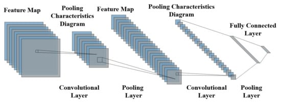
Figure 1.
Diagram of convolutional neural network.
The convolution layer is mainly divided into convolution and activation operations [18]. Assuming a layer with a total of N neurons, a convolution operation is performed between the feature map of the previous layer and the convolution kernel. The new feature matrix is then output by a specific activation function [19]. After the convolution layer, the expressive power of the model will be enhanced. Given a training sample set S, the convolution operation proceeds as follows.
The summation part of Equations (1) and (2) is equivalent to solving for a single cross−correlation term, where w is the weight and b is the bias. Zl and Zl+1 denote the convolutional input and output of layer l + 1, i.e., the feature map. Ll+1 is the size of Zl+1. Z(i,j) corresponds to the elements of the feature map. K, f, s0, and p denote the number of channels, the convolutional kernel size, the convolutional step size, and the number of padding layers of the feature map.
After the convolution of the input information, a ReLU activation function is used to perform a non−linear mapping of the output of each convolution kernel in the convolution layer to assist in the representation of complex features. The representation is as follows.
The expression for the ReLU activation function is as follows.
After feature extraction is completed in the convolution layer, the output feature map is transferred to the pooling layer for feature selection and information filtering. The pooling layer is also called the downsampling layer, and its most common methods include maximum pooling and average pooling. Its main function is to provide strong robustness, reduce the number of network parameters and prevent over−fitting. In this paper, maximum pooling is used to retain the overall features of the high−dimensional information as much as possible, which is represented as follows.
where f, s0, I and j have the same meaning as convolutional layers and p is a pre−specified parameter, where p→∞.
2.1.2. Long Short−Term Memory, LSTM (Recurrent Neural Network, RNN)
Long short−term memory networks are a special type of recurrent neural networks, which can be used to process sequential data. The self−looping structure of LSTM enables it to store temporal information about the inflow of memory units. It is very effective in learning long sequence dependence problems [20]. In order to overcome problems such as gradient explosion or gradient disappearance during training of traditional RNN models, three structures have been introduced in the LSTM to improve the RNN, namely forgetting gates, input gates, and output gates, respectively [21], as shown in Figure 2.
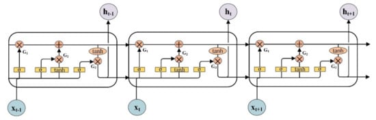
Figure 2.
Schematic diagram of LSTM neural network structure.
The mathematical expressions for the structures in the LSTM memory unit are as follows.
where ig represents the input gate, fg represents the forget gate, Og represents the output gate, xt represents the state of the memory cell at moment t, u represents the updated candidate information, and Ot is the final output information in the memory cell.
2.1.3. Deep−Learning Model Architecture
In this paper, a stacked CNN−LSTM deep hybrid neural network prediction model is developed. It consists of multiple one−dimensional convolutional and LSTM structures stacked on top of each other, with the input of the lower layer coming from the output of the previously hidden layer. The convolutional structure is used to extract spatial relationships at different levels from high−dimensional features (e.g., pressure and flow between different sources and users of the network). The gated loop structure is used to capture the temporal dynamics of the pipe network operational data (e.g., the trend data of a node feature in the pipe network over time). In order to use the stacked CNN−LSTM model for predicting changes in state parameters such as heat value at different supply metering nodes in the gas network, a predictor (consisting of two fully connected layers) is superimposed on the output layer of the model. In addition, the dropout technique from stochastic deactivation theory is introduced to ensure the generalization capability of the network. In other words, it means that some of the neurons in the neural network are randomly switched off before the fully connected layers to prevent overfitting of the model. As shown in Figure 3, the stacked CNN−LSTM structure and predictors constitute the entire deep−learning model.
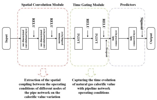
Figure 3.
Schematic diagram of deep−learning model structure.
2.2. Network Training
The deep−learning model needs to be periodically tuned and retrained with new data to ensure that the model can maintain good performance under changing operating conditions. To illustrate the logic and framework of the proposed method, the entire flow of the prediction method is shown in Figure 4.
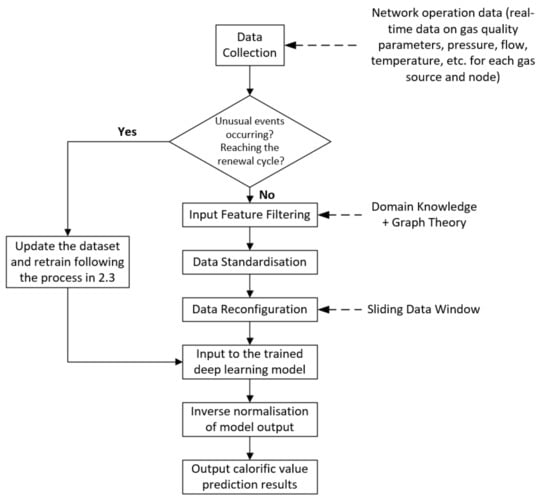
Figure 4.
The flowchart of dynamic prediction method of calorific value based on deep learning.
2.2.1. Data Reconfiguration
Before training the deep−learning model, the training data need to be reconstructed for the prediction model. In this paper, we used a sliding data window approach [22] to partition and reconstruct the virtual operational data of the natural gas pipeline system obtained in the previous section. Figure 5 illustrates the data update diagram for the sliding data window.
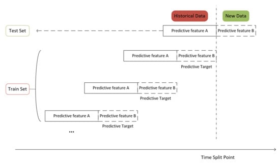
Figure 5.
Schematic diagram of sliding data window.
First, for historical data, we constructed one or more sets of data by intercepting data in different time windows. Then, each set of data was artificially divided into a historical window (corresponding to the solid part in Figure 5) and a future window (corresponding to the dashed part in Figure 5). Next, separate predictive features were constructed for each set of data, including historical features (predictive feature A) and future features (predictive feature B). At the same time, each set of data had a ‘future’ predictive target constructed from past time. Based on this reconstruction logic, we combined all the predictive features obtained as inputs to the model, such as historical operating data such as gas quality, pressure, flow, temperature, etc. for each gas source, pressure station, and customer node. We combined all prediction targets as model outputs, such as the calorific value or flow rate of gas at a downstream gas supply metering node for a certain time period in the future.
In addition, the length of the data window had an impact on the computational accuracy and efficiency of the prediction model. The longer the forecasting time, the greater the contribution to decision support provided by the pipeline operator. However, as uncertainty increases, this can lead to a reduction in forecast accuracy. Therefore, the length of the data window is often designed based on the actual application requirements and the experience of the analysts. Deep−learning models will collect new data at specific time intervals by the length of the data window and update the inputs by data window reconstruction.
2.2.2. Training Process and Assessment Indicators
This model is trained based on the BP algorithm of gradient descent [23,24] and the network parameters are iteratively updated while minimizing the prediction error by the Adam optimization algorithm [25]. In addition, the selection of the neural network hyperparameters has an impact on the prediction performance of the model. Here it is proposed to use a trial−and−error approach based on experience and grid search for optimization. Figure 6 illustrates the entire training process.
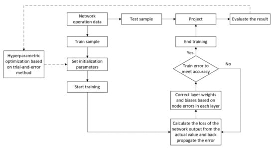
Figure 6.
The flowchart of training process.
The time series predictions of gas quality and state parameters for different gas supply metering sites in the study are regression problems. In order to better evaluate the differences between the model predictions and the benchmark values, four evaluation metrics, namely mean absolute error (MAE), root mean squared error (RMSE), mean absolute percentage error (MAPE), and regression coefficient of determination R2 were used as the four evaluation metrics for the proposed deep−learning models. The expressions for the four evaluation indicators are as follows.
- Mean absolute error (MAE):
- Root mean squared error (RMSE):
- Mean absolute percentage error (MAPE):
- Regression coefficient of determination R2:
where n is the number of samples, yi denotes the sample true value, ŷi denotes the model predicted value, and ȳi denotes the mean of the sample true values.
Among the above indicators, smaller values of MAE, RMSE, and MAPE indicate more accurate model prediction results, and a R2 value closer to 1 indicates a better fit of the regression model.
3. Case Study
This chapter applies the developed deep−learning model to the natural gas pipeline network structure for example validation. This is used to verify the predictive performance of the gas quality changes and the non−linear evolution of the system state in the natural gas pipeline network. The real−time operational data of the network required for model training is generated from TGNET simulations. The size of the input layer in a deep−learning model is determined by the dimensionality of the features in the input data. In this case, the input features are selected by combining domain knowledge with graph theory concepts. The structure of each hidden layer (i.e., the number of layers and the number of neurons in each layer) is determined by trial−and−error methods based on the prediction performance. The predicted output layers are the heat values of the gas supply metering nodes, etc.
In addition, we consider that the state parameters collected at different nodes of the pipe network vary significantly. To enhance the learning efficiency of the model, we normalized the data set under each feature separately according to Equation (3) to normalize the input data to within the range [0, 1]. The normalization method is as follows.
3.1. Data Preparation
In the process of collecting real−time operational data from pipeline networks, the lack of systematic planning of data platforms, inadequate monitoring equipment, and potential errors in the data storage process often result in insufficient data volumes, data anomalies, and large amounts of noise interference in the field [26]. To solve this problem, this study relies on the pipe network simulation software TGNET for data expansion.
From the information collected on−site, it has 4 gas sources. These include an LNG supply terminal and a UGS supply terminal, 2 compressor stations, and 31 customer demand points (including city gate stations, plants, power stations, and downstream outlets). There are a total of 35 pipelines with a total length of 553 km and diameters of 406.4–1016 mm. The network generally operates at pressures of 6–10 MPa. The topology of the gas pipeline network is shown in Figure 7. In the diagram, the red polygons represent the gas sources, the green polygons represent the various types of consumers, and the blue polygons represent the pressure stations, which are connected to each other by nodes.
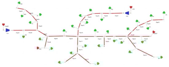
Figure 7.
Topological structure of natural gas pipeline networks.
To carry out the simulation, it is first necessary to set the initial and fixed boundary values for each component separately. These parameters are taken from the collected field operation data. In particular, the boundary condition control mode for the two main gas sources is pressure control, while the remaining sources and users are set to flow control mode. In addition, both pressure stations are set to the maximum outlet pressure control mode, which provides an outlet pressure maintained at set points of 10 (Supply1) and 9 Mpa (LNG), respectively.
In addition, to ensure that the operational data generated by the physical model were more closely matched to the actual production and operational characteristics, continuous time series data such as changes in the gas quality of each gas source and fluctuations in customer demand is one of the necessary boundary conditions for the dynamic simulation of the pipeline network. However, the dynamic behavior of gas sources in the network, such as gas quality changes and gas demand fluctuations, was not completely random. Rather, it was subject to a combination of physical process constraints and market characteristics. It is therefore not reasonable to generate such boundary conditions in a stochastic manner.
Taking these factors into account, the study is based on the relatively small amount of gas use flow data that has been collected on−site, and we resort to means such as time series feature analysis. The study generated continuous, complete time series of gas quality changes and gas use fluctuations that have approximate characteristics (fluctuation frequency, amplitude, period) to the actual fluctuation data. Monte Carlo simulations based on ARIMA model fitting analysis were carried out on the original series using the econometric toolbox of MATLAB R2021a. From this, we obtained the dynamic boundaries required for the reconfiguration model of the pipe network state.
Based on the above topology and boundary condition settings, a state reconstruction model of this natural gas pipeline network was constructed using TGNET. The simulation process was carried out according to the following principles and settings.
- (1)
- Under normal conditions, the system state and gas quality conditions will vary with fluctuations in gas source and demand;
- (2)
- The pressure and flow sensors record the system state at a given time interval (every 1 h in this study). The duration of the simulation is 10,000 h;
- (3)
- Gas quality tracking is switched on. The BWRS equation was chosen for the gas state equation.
Finally, the virtual operational data generated by the dynamic simulation is considered the actual operational parameters of the pipe network and used as the database for the next step of building the deep−learning model. In the latter empirical analysis, these parameters serve two purposes:
- (1)
- As training data for the deep−learning model;
- (2)
- As a reference base for the prediction results of the deep−learning model.
The initial information for each gas source in the network is shown in Table 1, which shows the variety of gas sources in the network and the significant differences between sources. In addition, due to the high variability of the LNG supply, the frequency of gas injection, and the real−time fluctuations of other gas sources within a certain range, this can lead to unusually complex gas mixing and gas quality fluctuations at local locations when the pipeline network is heavily tasked (e.g., during winter supply). Therefore, this is used as the initial conditions and dynamic boundary conditions for the TGNET hydraulic and thermal simulation to generate the demand fluctuation data, which is sourced in Figure 8.

Table 1.
Parameters of gas sources.
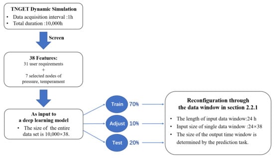
Figure 8.
Data sources.
In order to illustrate the reliability of the simulation results, the various characteristics of the generated dynamic boundary data were analyzed in comparison with the real data. Here, the user requirements of a node were used as an example. The statistical characteristics and temporal characteristics of the real and generated data are analyzed in Table 2 and Figure 9. The observation shows that the generated sequence data were cyclical to some extent. However, it was not a repetitive cycle, and it was able to simulate the changes in gas demand in the real world. At the same time, it exhibited similar characteristics to the real data in all analytical indicators. The distribution of the generated data tended to be more normal, except for the differences in the distributions of the two, and the smoothness of the series was better. Therefore, the dynamic simulation results based on the generated data could better reflect the dynamic evolution of the real network.
Table 2.
Comparison of statistical characteristics between original data and generated data.
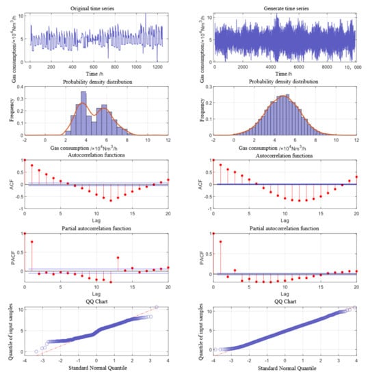
Figure 9.
Analysis of time series characteristics between original data and generated data.
3.2. Experiment Design
The convolutional module in the convolutional neural network and the gated recurrent unit in the long and short−term memory neural network were used for the deep extraction of spatially correlated and temporally evolved features during the operation of the pipe network. The spatial features were derived from pressure and flow data between different gas sources and users, while the temporal features were derived from the trend evolution data of the features of a node accumulated over time. In order to explore the predictive capability of the deep−learning models built into the method under different conditions, the following experimental scenarios were designed, respectively.
- (1)
- To demonstrate the superiority of the built deep−learning models over other advanced models (e.g., classical machine learning models, shallow neural networks, and single deep−learning models), we compared the prediction performance of the built deep−learning model (CNN−LSTM) with support vector machines (SVM), shallow BP neural networks (BPNN), convolutional neural networks (CNN), and LSTM recurrent neural networks (LSTM), respectively;
- (2)
- There is often a strong correlation between model prediction ability and prediction time. To demonstrate the prediction performance of CNN−LSTM models at different prediction time scales, we chose the prediction time window lengths of 2, 5, 8, 10, and 15 h for comparison experiments;
- (3)
- Generally speaking, field−collected data are noisy. To illustrate the effectiveness of the proposed method in dealing with different noise disturbances, we introduced five levels of artificial noise (i.e., ±0.5%, ±1.0%, ±1.5%, ±2.0%, ±2.5% Gaussian white noise) for comparison experiments;
- (4)
- There may be key data missing from the data collected in the field. In order to analyze the robustness of the model in response to situations such as missing data anomalies, we tested the prediction performance of the model under each of the five input data missing modes.
4. Results and Discussion
In this case, the network parameters of the model (i.e., the number of hidden layers and the number of neurons in each hidden layer, etc.) were optimized by tuning the parameters several times, and the finalized parameters were set as follows: the time−based convolution module contained two convolutional layers and one maximum pooling layer. The convolutional kernel size was 1 × 1, the number of neurons was [64, 32], and the activation function was ReLU. The temporal gating module contained two LSTM layers, the number of neurons was [300, 300], and the activation function was ReLU. The dropout layer parameter was set to 0.5, which meant that 50% of the neurons were randomly turned off. The output layer contained two fully connected layers. The first fully connected layer had 64 neurons, and the last layer had a number of neurons equal to the length of the prediction time. The activation function was Sigmoid. The model was trained using the Adam optimizer minimizing the mean squared error over 100 rounds, with a batch size of 250 and an initial learning rate of 0.001.
The models were trained and tested separately according to the parameter settings and experimental protocols described above, and the respective experimental results were analyzed, and detailed results are presented below.
4.1. Comparison of Prediction Performance of Different Models
In order to better illustrate the advantages of CNN−LSTM over SVR, BPNN, CNN, and LSTM models in capturing the spatio−temporal dynamics of complex gas mixing and transport processes in the pipeline network, the prediction task here was to predict the gas heat value of a customer (known from simulation results) with more severe and frequent gas quality fluctuations over the next 1 h. The hyperparameters of the different prediction models were carefully designed using a “trial−and−error” approach to ensure that the results are representative of their best capabilities. The parameters for each model are shown in Table 3.
Table 3.
The optimal parameters of different prediction models.
Figure 10 shows a comparison of the gas calorific value prediction results for the next 1 h from different models. It uses the four aforementioned error evaluation metrics as a benchmark for model prediction performance, and the results are shown in Table 4. From the figure and table, we can observe that this deep−learning model (CNN−LSTM) proposed in the method possessed higher accuracy and better fit compared to other benchmark models. It achieved a prediction accuracy of 99.89% for calorific values and was the only model with an R2 greater than 0.95. Figure 11 shows the CDF of the relative errors in the prediction results of the different models. It depicts the instability of the model prediction results due to the dynamics of the system state changes (caused by upstream gas quality changes and downstream user demand fluctuations). The results show that the established deep−learning model had better control over the prediction errors and the prediction performance was more reliable compared to the results of other models.
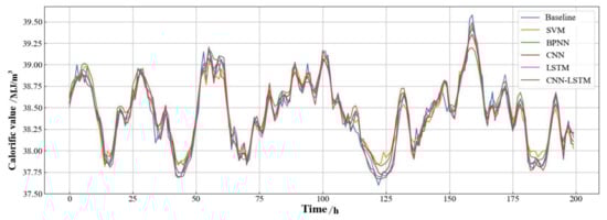
Figure 10.
Single−step prediction results of calorific value with different models.
Table 4.
Comparison for prediction performance with different models.
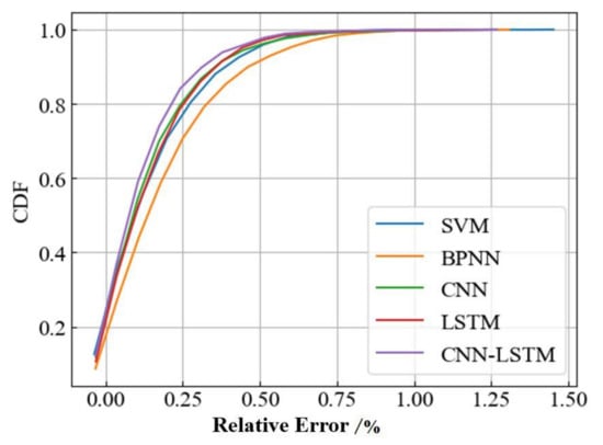
Figure 11.
Performance comparison based on the CDF of the relative error of prediction results.
4.2. Comparison of Prediction Performance at Different Time Scales
In general, longer prediction times can provide better decision support for gas quality analysis and metering management in pipeline networks. However, the size of the forecast output time also has a direct impact on the predictive capability of the model in the method. For this reason, the prediction task was tested by predicting the calorific value of the gas in the pipeline network for the next 2, 5, 8, 10, and 15 h respectively. Figure 12 shows the prediction of the gas calorific values by the deep−learning model built at different prediction time scales. It can be seen that as the prediction time increased, the prediction results beaome less accurate, and the fit became worse. This is because the strength of the relationship between the current and future states of the gas in the pipe network weakens with increasing prediction time, correspondingly making it more difficult for the neural network to learn this interrelationship.
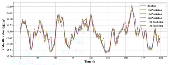
Figure 12.
Prediction results of calorific value under different time scales.
The results for each of the error evaluation metrics are displayed in Table 5 and the CDF for the relative error values is shown in Figure 13. From these results, we can observe that as the prediction time increases from 2 to 15 h, the values of the model MAE, RMSE, and MAPE change by a factor of nearly three. However, there was a more significant decrease in the R2 values of the model after 8 h. The difference in CDF between 8 and 5 h in the relative error CDF plot was greater than the difference between 5 and 2 h. This indicates that the deep−learning model was able to guarantee more accurate and reliable results for predictions within 5 h. In addition, with a prediction time of 15 h, the computation time of the deep−learning model built in this study was 1.3172 s, which was only 1% of the computation time of the physical simulation model (162.3357 s).
Table 5.
Comparison for prediction performance under different time scales.
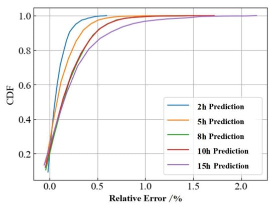
Figure 13.
Performance comparison based on the CDF of the relative error of prediction results.
4.3. Comparison of Prediction Performance with Different Input Noise
In this example, different levels of artificial noise were added to the numerical simulation results in order to illustrate the prediction model’s ability to make accurate predictions using noisy data. This was used as input to analyze the robustness of the hybrid model in response to data noise disturbances.
Figure 14 and Figure 15 show the CDF comparison of the predicted calorific value and the relative error of prediction for the next 2 h at different noise levels, respectively. From the figures, we can observe that there was a relatively significant decrease in the model prediction as the noise level increases. The results for each of the evaluation indicators are shown in Table 6. It can be seen that the values of the model MAE, RMSE, and MAPE increased by nearly four times at different noise levels. It reflects the fact that the average relative error of the model’s true predictive capability, although generally maintained at a low level, was considered unacceptable when this parameter was greater than 0.5% in terms of industry technical requirements. This suggests that the model’s predictions are unreliable when the noise level was above 1.5%. Furthermore, we can observe a very significant decrease in R2 values from 1.0% to 1.5% noise. This indicates that the model was not able to extract the spatial and temporal evolution of the gas state within the pipe network well when the noise disturbance is more severe. Therefore, by reducing the noise level to below 1.0%, the model can be effective in making predictions.
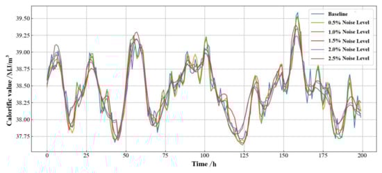
Figure 14.
Prediction results of calorific value under different noise levels.
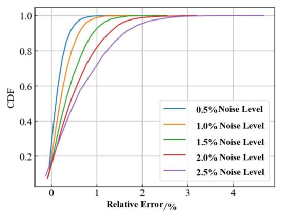
Figure 15.
Performance comparison based on the CDF of the relative error of prediction results.
Table 6.
Comparison for prediction performance under different noise levels.
4.4. Comparison of Prediction Performance under Different Input Deficiencies
As the current data platform in the field was not perfect, there were cases where data are missing, or key data measurements were missing at certain nodes during the data collection process. To further illustrate the robust performance of the model under different data missing conditions, the results of the 2 h heat value prediction will be compared based on five different sets of input data.
- DataA: All nodal pressure, air quality and demand data;
- DataB: All node pressure, air quality data, three missing demand data (compared to DataA);
- DataC: Pressure data for all nodes, missing data for three demands, gas quality data for one major gas source (compared to DataA);
- DataD: All nodal air quality data, missing three demand data, pressure data for three important nodes (compared to DataA);
- DataE: All node demand data, no pressure and temperament data (compared to DataA).
Comparisons of prediction accuracy for the five input data missing models are shown in Figure 16 and Figure 17. It can be visually observed from the graphs that the model maintained good prediction accuracy and stability of control over errors when some of the measurement data were missing less. For example, the prediction error results in Figure 16 for the missing Data B and Data C data model. However, when certain key data (e.g., pressure at some important driving nodes) were missing more, it was difficult for the model to fully extract and learn the dynamic characteristics of the non−linear process in the pipe network. This led to a significant reduction in both the fit and accuracy of the model predictions. This can also be seen in the gap between Data C and Data D in Figure 16 and the trend line in Figure 17.
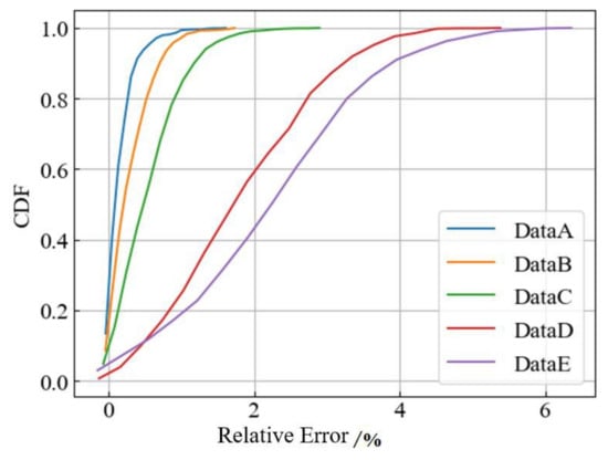
Figure 16.
Performance comparison based on the CDF of the relative error of prediction results.
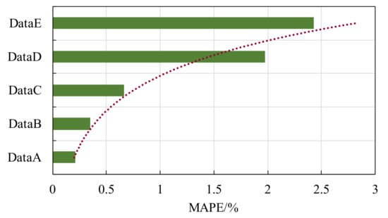
Figure 17.
Comparison for MAPE with different input data missing.
5. Conclusions
This paper presented a deep−learning−based dynamic prediction method for the calorific value of gas in large mixed gas pipeline systems. This method can be used to analyze in real−time the dramatic fluctuations in gas composition and calorific value due to gas quality differences and fluctuations in customer demand.
Numerical experiments show that: (1) The deep−learning model can effectively explore the unique physical characteristics and dynamic features of the pipeline network system. This method can quickly predict the dynamic changes of gas calorific value in the pipeline network based on real−time operational data such as pressure, flow rate, and gas quality parameters, with a prediction accuracy of over 99%. (2) Compared with the method based on physical simulation, this method can effectively reduce the computational burden and improve the efficiency of real−time analysis in the field while ensuring a certain prediction accuracy. (3) This method is able to maintain an accuracy of more than 97% when data noise interferes and some data such as pressure and flow rate at certain nodes are missing. This may provide a new approach to the dynamic assignment of calorific values to complex natural gas pipeline networks and the management of on−site metering.
In this experiment, the performance of the deep−learning model was highly dependent on the scale of the sample data. It was difficult to optimize the hyperparameters of the model as well as to control the output, which is a black−box in nature. In the future, the machine learning theory of controllable and interpretable industrial systems should be developed and combined, and then the construction method of the model should be determined according to the data characteristics and business needs of the actual application scenarios.
Author Contributions
Writing—original draft, J.H.; Writing—review & editing, Z.Y.; Supervision, Z.Y. and H.S.; Funding acquisition, H.S. All authors have read and agreed to the published version of the manuscript.
Funding
This work is supported by National Natural Science Foundation of China [grant number 51904316], and the research fund provided by China University of Petroleum, Beijing [grant number 2462021YJRC013].
Data Availability Statement
Data will be made available on request.
Conflicts of Interest
The authors declare no conflict of interest.
Nomenclature
| w | weight |
| b | bias |
| Zl, Zl+1+1 | convolutional input and output of layer l + 1 |
| Ll+1 | the size of Zl + 1 |
| Z(i,j) | the elements of the feature map |
| K | the number of channels |
| f | the convolutional kernel size |
| s0 | the convolutional step size |
| p | the number of padding layers |
| ig | the input gate |
| fg | the forget gate |
| Og | the output gate |
| xt | the state of the memory cell at moment t |
| u | the updated candidate information |
| Ot | the final output information in the memory cell |
| n | the number of samples |
| yi | the sample true value |
| ŷi | the model predicted value |
| ȳi | the mean of the sample true values |
References
- Huang, W.; Duan, J.; Chang, H.; Luo, Q.; Zhou, L.; Sun, Q. Construction of natural gas energy–measuring system in China: A discussion. Nat. Gas Ind. B 2022, 9, 33–40. [Google Scholar] [CrossRef]
- U.S. Department of Energy Office of Scientific and Technical Information. Natural Gas Monthly; U.S. Department of Energy Office of Scientific and Technical Information: Oak Ridge, TN, USA, 1991. [Google Scholar] [CrossRef]
- Ulbig, P.; Hoburg, D. Determination of the calorific value of natural gas by different methods. Thermochim. Acta 2002, 382, 27–35. [Google Scholar] [CrossRef]
- Wylie, E.B.; Stoner, M.A.; Streeter, V.L. Network: System transient calculations by implicit method. Soc. Pet. Eng. J. 1971, 11, 356–362. [Google Scholar] [CrossRef]
- Abbaspour, M.; Chapman, K.S. Nonisothermal transient flow in natural gas pipeline. J. Appl. Mech. 2008, 75, 031018. [Google Scholar] [CrossRef]
- Greyvenstein, G.P. An implicit method for the analysis of transient flows in pipe networks. Int. J. Numer. Methods Eng. 2002, 53, 1127–1143. [Google Scholar] [CrossRef]
- Li, C.; Jia, W.; Wu, X. A steady state simulation method for natural gas pressure—Relieving systems. J. Nat. Gas Sci. Eng. 2014, 19, 1–12. [Google Scholar] [CrossRef]
- Su, H.; Zio, E.; Zhang, J.; Chi, L.; Li, X.; Zhang, Z. A systematic data–driven Demand Side Management method for smart natural gas supply systems. Energy Convers. Manag. 2019, 185, 368–383. [Google Scholar] [CrossRef]
- Chalapathy, R.; Khoa, N.L.D.; Sethuvenkatraman, S. Comparing multi–step ahead building cooling load prediction using shallow machine learning and deep learning models. Sustain. Energy Grids Netw. 2021, 28, 100543. [Google Scholar] [CrossRef]
- Alzubaidi, L.; Zhang, J.; Humaidi, A.J.; Al–Dujaili, A.; Duan, Y.; Al–Shamma, O.; Santamaría, J.; Fadhel, M.A.; Al–Amidie, M.; Farhan, L. Review of deep learning: Concepts, CNN architectures, challenges, applications, future directions. J. Big Data 2021, 8, 53. [Google Scholar] [CrossRef]
- Chattopadhay, A.; Sarkar, A.; Howlader, P.; Balasubramanian, V.N. Grad–cam++: Generalized gradient–based visual explanations for deep convolutional networks. In Proceedings of the 2018 IEEE Winter Conference on Applications of Computer Vision (WACV), Lake Tahoe, NV, USA, 12–15 March 2018; pp. 839–847. [Google Scholar]
- Couliably, S.; Kamsu–Foguem, B.; Kamissoko, D.; Traore, D. Deep learning for precision agriculture: A bibliometric analysis. Intell. Syst. Appl. 2022, 16, 200102. [Google Scholar] [CrossRef]
- Nigam, A.; Garg, S.; Agrawal, A.; Agrawal, P. Crop yield prediction using machine learning algorithms. In Proceedings of the 2019 Fifth International Conference on Image Information Processing (ICIIP), Shimla, India, 15–17 November 2019; pp. 125–130. [Google Scholar]
- Hossain, E.; Khan, I.; Un−Noor, F.; Sikander, S.S.; Sunny, M.S.H. Application of big data and machine learning in smart grid, and associated security concerns: A review. IEEE Access 2019, 7, 13960–13988. [Google Scholar] [CrossRef]
- You, S.; Zhao, Y.; Mandich, M.; Cui, Y.; Li, H.; Xiao, H.; Fabus, S.; Su, Y.; Liu, Y.; Yuan, H.; et al. A review on artificial intelligence for grid stability assessment. In Proceedings of the 2020 IEEE International Conference on Communications, Control, and Computing Technologies for Smart Grids (SmartGridComm), Tempe, AZ, USA, 11–13 November 2020; pp. 1–6. [Google Scholar]
- Kanjo, E.; Younis, E.M.; Ang, C.S. Deep learning analysis of mobile physiological, environmental and location sensor data for emotion detection. Inf. Fusion 2019, 49, 46–56. [Google Scholar] [CrossRef]
- Wang, W.; Tang, Z.; Chen, Y.; Sun, Y. Parity recognition of blade number and manoeuvre intention classification algorithm of rotor target based on micro–Doppler features using CNN. J. Syst. Eng. Electron. 2020, 12, 18–26. [Google Scholar]
- Verstraete, D.; Ferrada, A.; Droguett, E.L.; Meruane, V.; Modarres, M. Deep learning enabled fault diagnosis using time–frequency image analysis of rolling element bearings. Shock. Vib. 2017, 2017, 5067651. [Google Scholar] [CrossRef]
- Schmidhuber, J. Deep learning in neural networks: An overview. Neural Netw. 2015, 61, 85–117. [Google Scholar] [CrossRef]
- Su, H.; Zio, E.; Zhang, J.; Xu, M.; Li, X.; Zhang, Z. A hybrid hourly natural gas demand forecasting method based on the integration of wavelet transform and enhanced Deep–RNN model. Energy 2019, 178, 585–597. [Google Scholar] [CrossRef]
- Xiao, Y.; Yin, H.; Zhang, Y.; Qi, H.; Zhang, Y.; Liu, Z. A dual–stage attention–based Conv–LSTM network for spatio–temporal correlation and multivariate time series prediction. Int. J. Intell. Syst. 2021, 36, 182–213. [Google Scholar] [CrossRef]
- Zhou, D.; Gao, F.; Breaz, E.; Ravey, A.; Miraoui, A. Degradation prediction of PEM fuel cell using a moving window based hybrid prognostic approach. Energy 2017, 138, 1175–1186. [Google Scholar] [CrossRef]
- Rumelhart, D.E.; Hinton, G.E.; Williams, R.J. Learning representations by back–propagating errors. Nature 1986, 323, 533–536. [Google Scholar] [CrossRef]
- Ruder, S. An overview of gradient descent optimization algorithms. arXiv 2016, arXiv:1609.04747. [Google Scholar]
- Kingma, D.P.; Ba, J. Adam: A method for stochastic optimization. arXiv 2014, arXiv:1412.6980. [Google Scholar]
- Li, G.; Wang, F.; Pi, X.; Liu, H. Optimized application of geology–engineering integration data of unconventional oil and gas reservoirs. China Pet. Explor. 2019, 24, 147. [Google Scholar]


Disclaimer/Publisher’s Note: The statements, opinions and data contained in all publications are solely those of the individual author(s) and contributor(s) and not of MDPI and/or the editor(s). MDPI and/or the editor(s) disclaim responsibility for any injury to people or property resulting from any ideas, methods, instructions or products referred to in the content. |
© 2023 by the authors. Licensee MDPI, Basel, Switzerland. This article is an open access article distributed under the terms and conditions of the Creative Commons Attribution (CC BY) license (https://creativecommons.org/licenses/by/4.0/).