A Comprehensive Multi-Factor Method for Identifying Overflow Fluid Type

Abstract

Accurate identification of overflow fluid types facilitates timely and effective handling of onsite overflow accidents. Research into identifying the type of overflow fluid is limited, and there are only simple calculation models that do not consider enough effects; additionally, accuracy needs to be improved and the identification method is not perfect. If there is no drilling data, it is impossible to identify the overflow fluid. Therefore, this paper modifies the density calculation model of overflow fluid by considering the influence of the temperature, pressure field, and two-phase flow model, making the calculation result more accurate and universal, and puts forward a comprehensive method for auxiliary identification based on gas logging interpretation. This paper uses the gas state equation to verify the accuracy of the overflow density model; after verification using data from more than 20 overflowing wells, the method was found to be practical and had an accuracy rate of more than 90%. Thus, this study and the proposed method can provide guidance for dealing with overflow accidents in the field and any follow-up research.

1. Introduction

In recent years, oil–gas exploration and development have been moving towards the deep stratum [1]. Drilling in a deep stratum is extremely difficult and accidents occur–for instance, wellbore overflow and circulation loss because reservoirs in deep stratum have complicated geological conditions under high temperature and high pressure, which are difficult to recognize [2]. Therefore, in order to select the proper well-killing method and deal with overflow accidents in a timely manner, it is first necessary to identify the type of overflow fluid. When an overflow occurs, the engineers usually identify the fluid based on work experience, which is often inaccurate, and errors in identification can lead to well-killing failures [3,4,5,6,7].

Of the many relevant papers, there are only a few studies that identify the type of overflow fluid. Only a simple calculation model exists, which can calculate the overflow fluid density quantitatively based on the U-tube principle by using drilling parameters (overflow amount, standpipe pressure, casing pressure, etc.) and identify the fluid by density–for instance, when ρ is less than 0.36 g/cm³, the fluid is gas. However, this model does not consider the influence of the temperature and pressure field and the two-phase flow model, so the results are non-universal and error-prone. When complete drilling data is not available, the model cannot be used, which is highly limiting [3,8,9]. The gas logging interpretation method is commonly used in oil and gas exploration and development engineering, and the fluid properties of the reservoir are determined by drawing the diagram of gas logging data or by using ratio methods, including the Pixler method, 3H ratio method, simple parameter method, methane correction method, etc., which have not been previously used to identify overflow fluid types [10,11,12,13,14,15,16]. On the basis of previous research, this paper proposes a multi-factor comprehensive method for identifying overflow fluid, including the overflow fluid density calculation correction method and the gas logging interpretation method. This paper considers the influence of temperature, pressure, and the two-phase flow model to modify the traditional overflow fluid density calculation model, quantitatively calculate the density, and perform auxiliary qualitative identification based on gas logging interpretations.

The next section introduces the traditional overflow fluid identification method and its shortcomings, and then introduces the comprehensive multi-factor method proposed in this paper. Section 4 uses the method proposed in this paper to calculate examples and verify the calculation model. Section 5 and Section 6 analyze the influencing factors and summarize the full paper. This paper has guiding significance for identifying the type of overflow fluid, dealing with overflow accidents onsite, and the subsequent research.

2. Traditional Overflow Fluid Identification Method and Its Deficiencies

Through analysis of the literature, it was found that there are three main methods for identifying overflow fluid: (1) identifying the overflow fluid by the field experience method; (2) calculating the density of the overflow fluid through the classical model and identifying the overflow fluid by density; (3) identifying the type of formation fluid by gas logging interpretation.

2.1. Empirical Method

When overflow occurs, engineers identify the type of overflow fluid based on work experience. If a gas kick occurs, the variability of casing pressure is much greater than the variability with an oil or water kick. If there is no oil slick in the mud back out, the overflow fluid can be determined to be water, and vice versa. This method is based on the experience of the engineers and so it is often inaccurate.

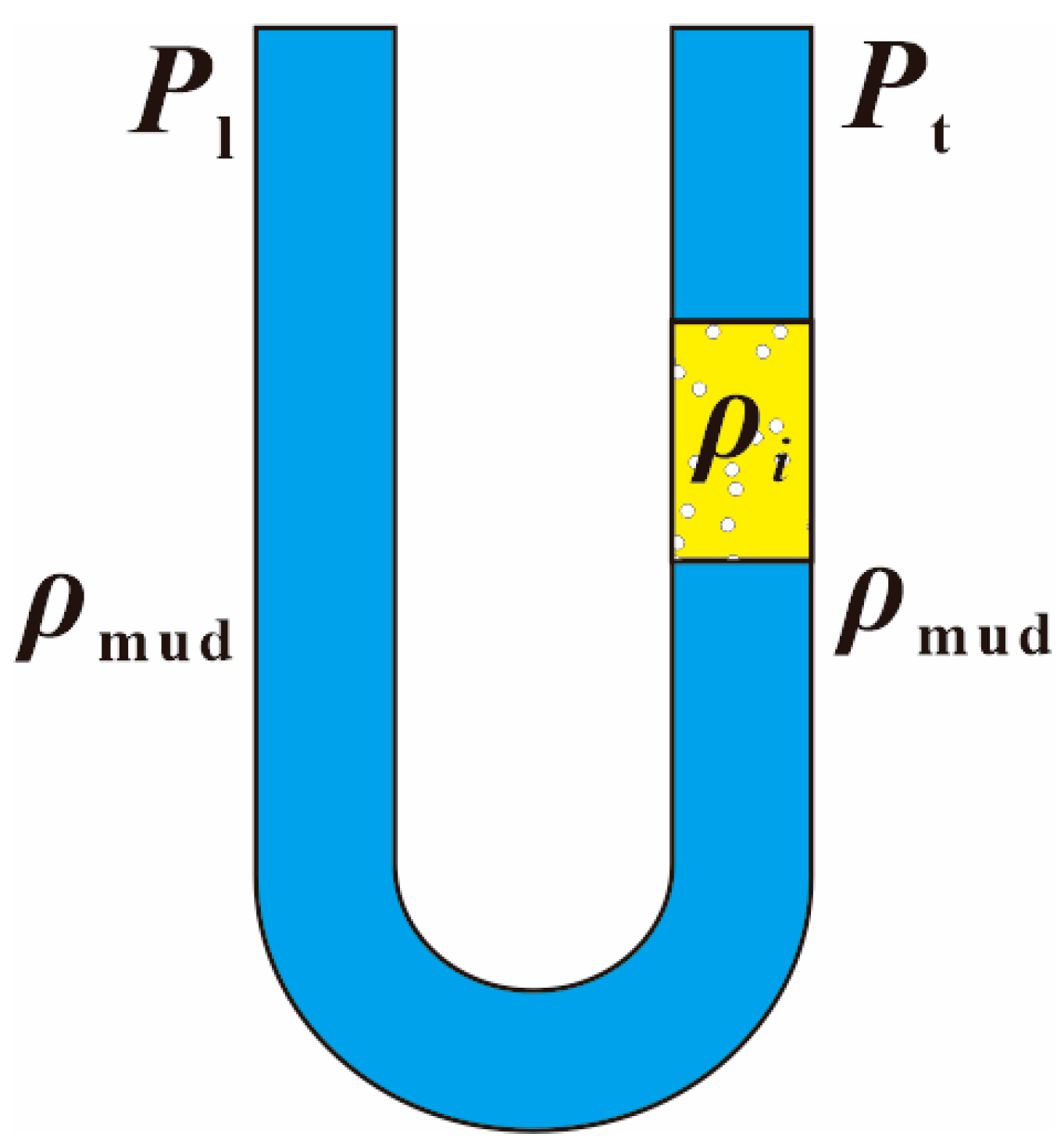
2.2. Classical Density Model

This method is derived from the wellbore U-tube model to calculate the overflow fluid density, to then identify the liquid type by density. In this method, it is assumed that after the overflow fluid kicks the wellbore, it is a continuous fluid in the wellbore. The calculation model is shown in Figure 1. The pressure relationship in the pipe is shown in Equation (1) [3,9].

$$P={\rho }_{\mathrm{mud}}gH+P_{\mathrm{l}}={\rho }_{i}g{H}_{\mathrm{o}}+P_{\mathrm{t}}+{\rho }_{\mathrm{mud}}g(H-H_{\mathrm{o}})$$

(1)

where ${\rho }_{\mathrm{mud}}$ is drilling fluid density, g/cm³; ${\rho }_i$ is overflow fluid density, g/cm³; $H$ is measured depth, m; $P_{\mathrm{l}}$ is standpipe pressure during well closing, MPa; $P_{\mathrm{t}}$ is casing pressure during well closing, MPa; $H_{\mathrm{o}}$ is the height of the overflow fluid section, m.

The height of the overflow fluid can be calculated by the overflow volume, the equation for which is:

$$H_{\mathrm{o}}=\frac{V_{\mathrm{o}}}{V_{\mathrm{a}}}H$$

(2)

where $V_{\mathrm{o}}$ is the overflow volume, m³; $V_{\mathrm{a}}$ is the volume of annular space, m³. Plugging Equation (2) into Equation (1) allows the estimation of the density of the overflow fluid.

$${\rho }_i={\rho }_{\mathrm{mud}}-\frac{(P_{\mathrm{t}}-P_{\mathrm{l}})V_{\mathrm{a}}}{0.00981H{V}_{\mathrm{o}}}$$

(3)

The density of the overflow fluid can be calculated by Equation (3); then, the fluid type can be identified by the difference in its density. The method is shown in

Table 1. Criteria for the type of overflow fluid.

Overflow Fluid Density	Overflow Fluid Type
ρ < 0.36 g/cm3	Gas
ρ = 0.37–0.60 g/cm3	Gas and oil mixture
ρ = 0.61–0.92 g/cm3	Oil or water and oil mixture
ρ > 0.92 g/cm3	Water or saltwater

.

The classical model does not consider the influence of the temperature, pressure field, and two-phase flow model on the calculation. Therefore, the calculation results are inaccurate and have certain limitations, and this method cannot be used without the complete drilling parameters.

2.3. Gas Logging Interpretation Methods

These methods are applied in oil–gas field development engineering to identify the type of fluid in the target stratum based on the gas logging interpretation. The type of overflow fluid can be identified by drawing diagrams or calculating the ratio of hydrocarbons based on the gas logging data during the period of the overflow. The identification methods include the Pixler method, triangle diagram method, 3H ratio method, etc. These methods cannot quantitatively calculate the overflow fluid density but can only identify it qualitatively; when there are many overflow formations in the downhole, if there is no data during the overflow period, these methods are not accurate [10,11,12,13,14,15,16].

3. Comprehensive Multi-Factor Method

After analyzing the above methods and their shortcomings, this study proposes a comprehensive multi-factor method to identify overflow fluid types, including the calculation correction method of overflow fluid density and the comprehensive analysis method based on the gas logging interpretation.

3.1. Calculation Correction Method of Overflow Fluid Density

In order to calculate the density of the overflow fluid more accurately in the deep stratum, the calculation model should first be modified by considering the influence of the temperature, pressure field, and two-phase flow model.

3.1.1. The Influence of Temperature and Pressure

The overflow fluid density in shallow wells can be obtained by using the classic model because the pressure and temperature have little effect on the density of the overflow fluid. However, there are higher temperatures (close to 200 °C) and pressures (about 100 MPa) in the deep stratum. In this situation, the overflow fluid density will change significantly. Therefore, in order to accurately calculate the density, it is necessary to consider the influence of the temperature and pressure fields [17].

Methods of calculating the wellbore temperature field have been proposed in many studies and are not the focus of this study; to simplify the calculation, in this study, the wellbore temperature field is calculated using the geothermal gradient [18,19], assuming that the surface temperature is 26.67 °C and the ground temperature gradient is 3 °C/100 m. The pressure field is calculated as follows. As shown in Figure 2, the drill string and the annular space are divided into ‘n’ calculation elements on average, and the length of each element is $h$. Assuming that each section is very short, the temperature, pressure, density, and volume fraction changes in this section of the wellbore can be ignored, thus, it is considered to be unchanged in each element [20,21]. Take the formation element $\Delta H$; the pressure of the element formation is: $P_1=P_0+{\rho }_1\mathrm{g}\Delta H$. In this equation, $P_0$ is the pressure of the upper formation element; ${\rho }_1$ is the density of drilling fluid at the corresponding temperature and pressure of this formation element; $P_2=P_1+{\rho }_2\mathrm{g}\Delta H$ is the pressure of the next formation element. The pressure of the nth formation element is $P_{\mathrm{n}}=P_{\mathrm{n}-1}+{\rho }_{\mathrm{n}}\mathrm{g}\Delta H$. Therefore, the pressure of each formation element can be calculated by using equations from the wellhead casing pressure [22].

Temperature and pressure do not affect shut-in casing pressure, shut-in standpipe pressure, well depth, the volume of annular space, and overflow volume in Equation (3); however, they do affect the density of the downhole drilling fluid. There are two main mathematical models for the downhole drilling fluid density calculation: the empirical density model and the composite density model [22].

(1)

Empirical density model

The empirical model is obtained from the analysis of a large number of experimental results; the downhole drilling fluid density can be calculated only by conducting a limited number of experiments on the drilling fluid used to determine the relevant parameters in the empirical model. The empirical density model is as follows:

$$\rho ={\rho }_0{e}^{a(P-P_0)+b{(P-P_0)}^2+c(T-T_0)+d{(T-T_0)}^2+e(P-P_0)(T-T_0)}$$

(4)

where ${\rho }_0$ is the drilling fluid density under $T_0$ and $P_0$, g/cm³; $T$, $P$ are the temperature and pressure of the drilling fluid during the experiment; $a$, $b$, $c$, $d$, $e$ are the drilling fluid characteristic constants; $T_0$, $P_0$ are normal temperature and pressure.

(2)

Composite density model

The composite density model considers that the drilling fluid is composed of components such as the water phase, oil phase, solid phase, and weighted substances. When the variation law of high temperature and high pressure of a single component is determined, a composite model for predicting the drilling fluid density can be obtained as follows:

$${\rho }_{\left(P,T\right)}=\frac{{\rho }_i}{1+f_{\mathrm{o}}\left(\frac{{\rho }_{\mathrm{o}}}{{\rho }_{\mathrm{o},\left(P,T\right)}}-1\right)+f_{\mathrm{w}}\left(\frac{{\rho }_{\mathrm{w}}}{{\rho }_{\mathrm{w},\left(P,T\right)}}-1\right)}$$

(5)

where ${\rho }_{\mathrm{o}}$ is the oil phase density of drilling fluid; ${\rho }_{\mathrm{w}}$ is the water phase density of drilling fluid; $f_{\mathrm{o}}$ is the oil phase volume fraction; $f_{\mathrm{w}}$ is the water phase volume fraction; ${\rho }_{\mathrm{o},\left(P,T\right)}$ is the density of the oil phase volume under high temperature and high pressure; ${\rho }_{\mathrm{w},\left(P,T\right)}$ is the density of the water phase under high temperature and high pressure.

The numerator in Equation (5) is the initial drilling fluid density:

$${\rho }_i={\rho }_{\mathrm{o}}{f}_{\mathrm{o}}+{\rho }_{\mathrm{w}}{f}_{\mathrm{w}}+{\rho }_{\mathrm{s}}{f}_{\mathrm{s}}+{\rho }_{\mathrm{c}}{f}_{\mathrm{c}}$$

(6)

where ${\rho }_{\mathrm{o}}$ is the oil phase density of the drilling fluid; ${\rho }_{\mathrm{w}}$, is the water phase density of the drilling fluid; ${\rho }_{\mathrm{s}}$ is the solid phase density of drilling fluid; ${\rho }_{\mathrm{c}}$ it the chemical additive density, $f_{\mathrm{o}}$ is the oil phase volume fraction; $f_{\mathrm{w}}$ is the water phase volume fraction; $f_{\mathrm{s}}$ is the solid phase volume fraction; $f_{\mathrm{c}}$ is the chemical additive volume fraction.

If the drilling fluid is composed of a single-liquid-phase (oil or water) and a solid phase, then Equation (5) can be converted into:

$${\rho }_{\left(P,T\right)}=\frac{{\rho }_{0(p_0,T_0)}}{1+\lambda \left(\frac{{\rho }_{f(p_0,T_0)}}{{\rho }_{f\left(P,T\right)}}-1\right)}$$

(7)

where ${\rho }_{f(p_0,T_0)}$ is the density of the liquid phase in the drilling fluid under the normal pressure and temperature; ${\rho }_{f\left(P,T\right)}$ is the density of the liquid phase in the drilling fluid under pressure P and temperature T.

The calculation model of the overflow fluid density considering the temperature and pressure is as follows.

The equation for calculating the bottom hole pressure through the annular space after shut-in is as follows:

$$P={\displaystyle \sum _{i=1}^k{\rho }_{mi}g}h+{\displaystyle \sum _{i=k}^n({\rho }_{mi}{f}_{mi}+{\rho }_{in}{f}_{ini})g}h+P_t$$

(8)

where ${\rho }_{mi}$ is the drilling fluid density in the annular space of the element i, g/cm^3; ${\rho }_{in}$ is the density of the kick fluid, g/cm³, $f_{mi}$ is the volume fraction of the drilling fluid in the annular space of the element i; $f_{ini}$ is the volume fraction of the kick fluid in annular space of the element i; $k$ is the element number at the interface of the single-phase region and the two-phase region; $P_t$ is the casing pressure during well closing, MPa.

The equation for calculating the bottom hole pressure through the drill string after shut-in is as follows:

$$P={\displaystyle \sum _{i=1}^n{\rho }_{mi}g}h+P_{\mathrm{l}}$$

(9)

where ${\rho }_{mi}$ is the drilling fluid density of the drill string in the element i, g/cm³; $P_{\mathrm{l}}$ is standpipe pressure during well closing, MPa.

Equations (8) and (9) can be combined to calculate the density of the overflow fluid as follows:

$${\rho }_{in}=\frac{({\displaystyle \sum _{i=1}^n{\rho }_{lmi}-{\displaystyle \sum _{i=1}^k{\rho }_{tmi}-{\displaystyle \sum _{i=k}^n{\rho }_{tmi}{f}_{mi}}}})gh+P_{\mathrm{l}}-P_{\mathrm{t}}}{{\displaystyle \sum _{i=k}^n{f}_{ini}gh}}$$

(10)

where ${\rho }_{tmi}$ is the drilling fluid density in the annular space of the element i, g/cm³;${\rho }_{lmi}$ is the drilling fluid density in the drill string of the element i, g/cm³; ${\rho }_{in}$ is the density of the kick fluid, g/cm³; $f_{mi}$ is the drilling fluid volume fraction in annular space of the element i; $f_{ini}$ is the kick fluid volume fraction in annular space of the element i; $k$ is the element number at the interface of the single-phase region and the two-phase region; $P_{\mathrm{t}}$ is casing pressure during well closing, MPa; $P_{\mathrm{l}}$ is standpipe pressure during well closing, MPa.

The previously calculated data is substituted into Equation (10) to modify the density of the overflow fluid using the iterative method from wellhead to bottom hole; then the type of fluid is identified using Table 1.

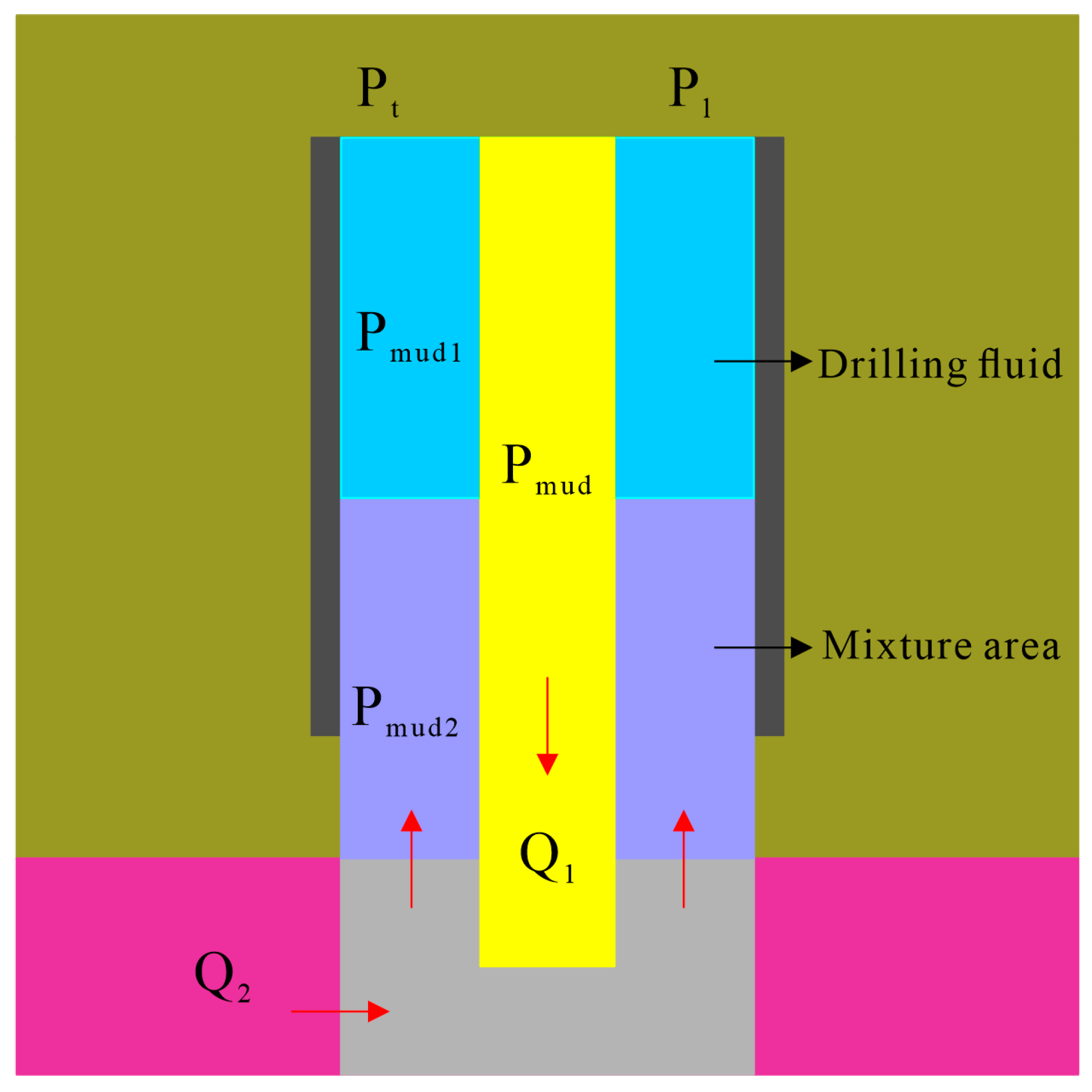
3.1.2. The Influence of the Two-Phase Flow Model

When the overflow fluid is identified to be gas, the gas is distributed in a two-phase flow pattern in the annular space after kicking the wellbore, which cannot be completely equivalent to the gas column, and is influenced by gas slippage expansion and gas migration. Therefore, the two-phase flow model is used to simulate the distribution of the gas–liquid two-phase flow in the wellbore during the overflow period. The density of the mixing section after the gas kick is calculated based on the void fraction during the overflow period, and the overflow fluid density calculation is corrected accordingly [23].

As shown in Figure 3, when it is judged as a gas kick, it is assumed that only part of the drilling fluid in the annular space is contaminated by the kicking fluid, which is the mixed drilling fluid, with the other part being solely drilling fluid. Then, considering the two-phase flow model, the wellbore U-tube principle equation is as follows:

$$P=P_{\mathrm{mud}1}+P_{\mathrm{mud}2}+P_{\mathrm{t}}=P_{\mathrm{mud}}+P_{\mathrm{l}}$$

(11)

$$P_{\mathrm{mud}1}={\rho }_{\mathrm{mud}}\mathrm{g}\left(H-H_{\mathrm{o}}\right)$$

(12)

$$P_{\mathrm{mud}2}=\left[\varphi {\rho }_{\mathrm{mud}}+\left(1-\varphi \right){\rho }_g\right]g{H}_{\mathrm{o}}$$

(13)

$$P_{\mathrm{mud}}={\rho }_{\mathrm{mud}}gH$$

(14)

In these equations, $P_{\mathrm{mud}1}$ is the pressure of the single-phase drilling fluid in the annular space, MPa, $P_{\mathrm{mud}2}$ is the pressure of the mixed drilling fluid in the annular space, MPa, ${\rho }_{\mathrm{g}}$ is the density of overflow fluid, g/cm³, $\varphi$ is the void fraction.

The calculation model of overflow fluid density considering the two-phase flow model is obtained by deduction, as shown in Equation (15).

$${\rho }_{\mathrm{g}}=\frac{({\displaystyle \sum _{i=1}^n{\rho }_{lmi}-{\displaystyle \sum _{i=1}^k{\rho }_{tmi}-{\displaystyle \sum _{i=k}^n{\rho }_{tmi}{f}_{mi}}}})gh+P_{\mathrm{l}}-P_{\mathrm{t}}}{{\displaystyle \sum _{i=k}^n\varphi gh}}$$

(15)

From the above equations, the corresponding pressure is calculated by the void fraction of each formation element; then, ${\rho }_g$ can be known.

3.2. The Gas Logging Comprehensive Analysis Method

In the gas logging comprehensive analysis method, one must first determine the time at which the overflow occurs. Determining the time when the overflow occurs is very important for extracting drilling parameters and gas logging data during the overflow period, as well as for calculating the average overflow kick rate and the void fraction. After a period of overflow, which is reflected in the drilling parameters, we only need to find the drilling parameter that first changed to confirm the approximate time of the overflow.

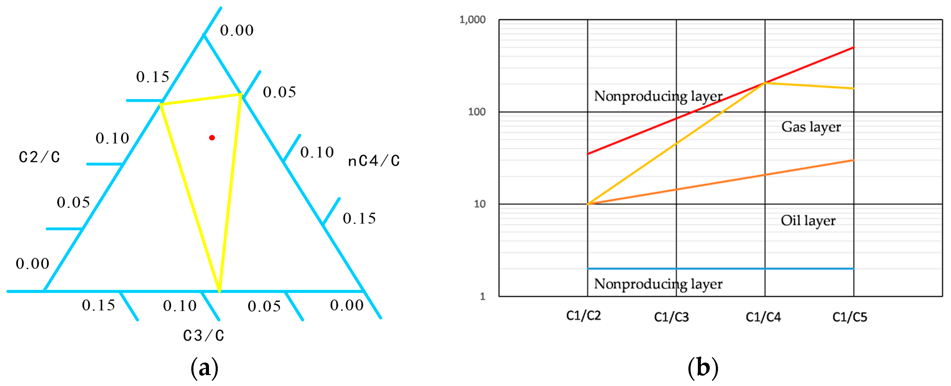
3.2.1. The Triangle Diagram Method

The triangle diagram method is to draw a triangle (as shown in Figure 4a) with three data points of the ratio of C₂, C_3, and C₄ to total hydrocarbons, and to judge the properties of the reservoir fluid according to the size and shape of the triangle [14,24]. The judging criteria are shown in

Table 2. The triangle diagram method judgment criteria.

The Internal Triangle Type	Reservoir Properties
An equilateral triangle	Gas layer
An inverted triangle	Oil layer
A large triangle (the border length ratio is greater than 100%)	Dry gas or the oil and gas ratio is very low
A small triangle (the border length ratio is less than 25%)	Wet gas or the oil and gas ratio is very high
The intersection of the inner triangle vertex and the vertex of the outer triangle is distributed in the internal triangle	Production capacity
The intersection of the inner triangle vertex and the vertex of the outer triangle is distributed outside the internal triangle	No production capacity

.

3.2.2. The Pixler Method

The Pixler method is used to evaluate the type of reservoir based on a statistical analysis of the hydrocarbon ratio data of the gas component in the reservoir. This study draws on this method to identify the type of overflow fluid by using the gas logging data of the overflow start time to draw a Pixler chart (as is shown in Figure 4b). The identification methods are as follows: The ratio of C₁/C₂ identifies the formation properties; when C₁/C₂ is less than 2, there is a dry formation. Generally, only C₁ in the reservoir indicates that the reservoir is a dry gas formation, unless the C₁ content is too high, which may be a brine layer. If the ratio of any hydrocarbon is lower than the ratio of the previous hydrocarbon, there is a non-production layer. The ratio of the hydrocarbon values to the line is positively inclined to indicate that there is a production layer, and the negative slope indicates an aquifer [11,15].

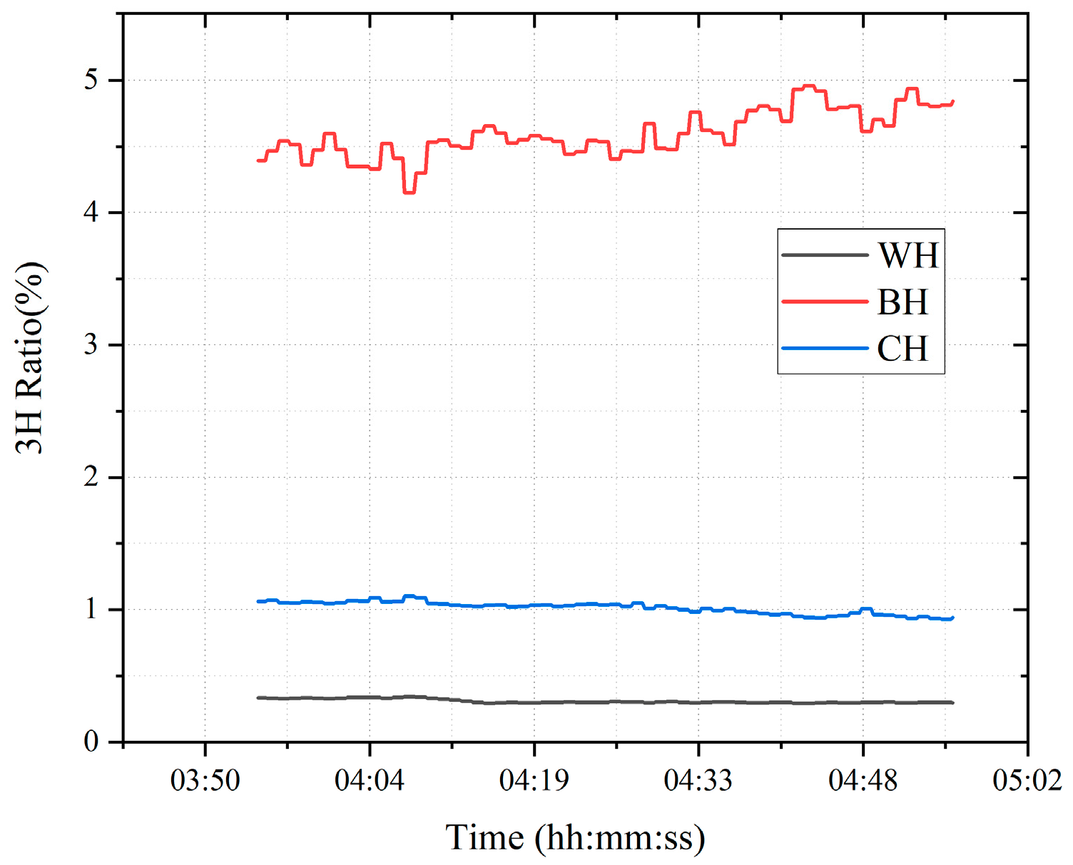
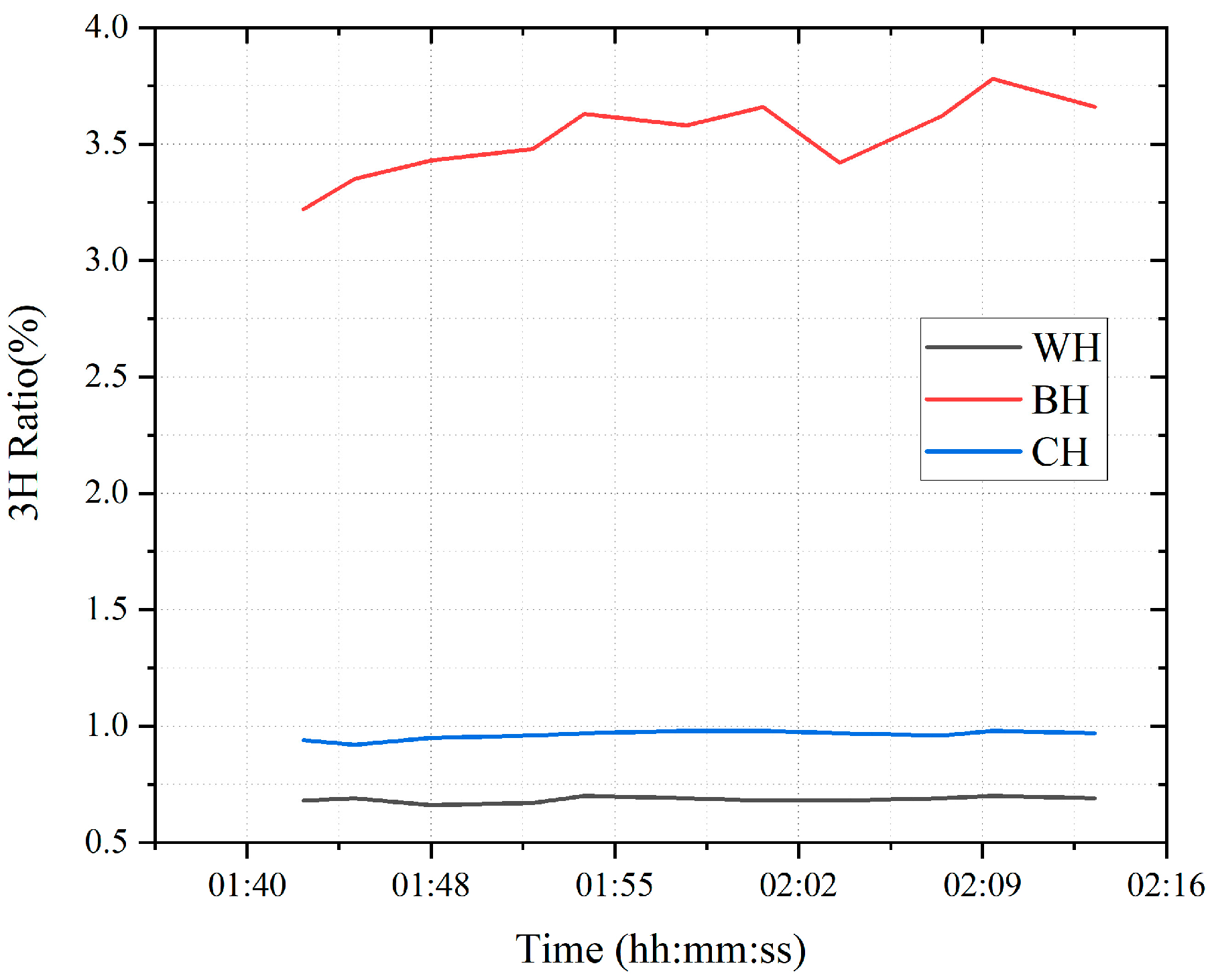
3.2.3. 3H Ratio Method

The psychrometric ratio, equilibrium ratio, and characteristic ratio (3H ratio) of hydrocarbon values from different components can be calculated by gas logging data to identify the type of overflow fluid [11]. The equations of the 3H ratio are shown below:

$$W_{\mathrm{h}}=\frac{C_2+C_3+C_4+C_5}{C_1+C_2+C_3+C_4+C_5}$$

(16)

$$B_{\mathrm{h}}=\frac{C_1+C_2}{C_3+C_4+C_5}$$

(17)

$$C_{\mathrm{h}}=\frac{C_4+C_5}{C_3}$$

(18)

$${\rho }_{\mathrm{g}}=\frac{({\displaystyle \sum _{i=1}^n{\rho }_{lmi}-{\displaystyle \sum _{i=1}^k{\rho }_{tmi}-{\displaystyle \sum _{i=k}^n{\rho }_{tmi}{f}_{mi}}}})gh+P_{\mathrm{l}}-P_{\mathrm{t}}}{{\displaystyle \sum _{i=k}^n\varphi gh}}$$

(19)

The following methods, as

Table 3. 3H ratio method judgment criteria.

3H Ratio	Type of the Fluid
$W_{\mathrm{h}}$ < 0.5	Light-associated gas, basically no productivity
$W_{\mathrm{h}}$ > 40	Heavy oil or residual oil, and low productivity
$W_{\mathrm{h}}$ < 0.5 and $B_{\mathrm{h}}$ > 100	Extremely light dry gas, unprofitable
0.5 < $W_{\mathrm{h}}$ < 17.5, $W_{\mathrm{h}}$ < $B_{\mathrm{h}}$ < 100	Recoverable gas
0.5 < $W_{\mathrm{h}}$ < 17.5, $B_{\mathrm{h}}$ < $W_{\mathrm{h}}$	Recoverable oil with a high gas–oil ratio
17.5 < $W_{\mathrm{h}}$ < 40, $B_{\mathrm{h}}$ < $W_{\mathrm{h}}$	Recoverable oil
0.5 < $W_{\mathrm{h}}$ < 17.5, $B_{\mathrm{h}}$ < $W_{\mathrm{h}}$, $C_{\mathrm{h}}$ < 0.5	Recoverable wet gas or condensate oil
0.5 < $W_{\mathrm{h}}$ < 17.5, $B_{\mathrm{h}}$ < $W_{\mathrm{h}}$, $C_{\mathrm{h}}$ > 0.5	Recoverable oil with a high gas–oil ratio

shows, can be used to identify the type of overflow fluid.

Here, the gas logging data during the overflow period of Well B is extracted and added into Equations (16)–(18) to calculate the 3H ratio during the overflow period; then, a 3H ratio diagram is drawn, as shown in Figure 5. $W_{\mathrm{h}}$ is about 0.2, $B_{\mathrm{h}}$ is about 4.5, and $C_{\mathrm{h}}$ is about 1. Referring to the identification method, Well B has basically no productivity and very light associated gas, which is consistent with the actual test results.

3.2.4. Comprehensive Analysis Method of Overflow Fluid Types Based on Gas Logging Interpretation

According to the characteristics and judgment scope of different gas logging interpretation methods, the authors established a comprehensive analysis method to assist in identifying the type of overflow fluid and determining the approximate range of overflow fluid density. If both the drilling parameters and gas logging data during the overflow period can be obtained, they can be verified against each other.

(1)

Identification of water and saltwater layers

When identifying the type of overflow fluid with the gas logging interpretation method, it is first necessary to determine whether the overflow formation is a water layer. Unlike the Pixler method, the triangular diagram method and the 3H ratio method cannot judge water layers and saltwater layers, thus, the Pixler plate method is used to determine whether the formation is a water layer. If the overflow formation is a water layer, the overflow fluid density is considered to be approximately 1.00 g/cm³; if it is a saltwater layer, the density is considered to be approximately 1.15 g/cm³.

(2)

Identification of oil and gas layers

Since the Pixler method can only distinguish oil layers and gas layers, it is difficult to determine the range of the overflow fluid density. The triangular diagram method and the 3H ratio method can further distinguish the properties of the oil layers and gas layers, which can narrow the range of the overflow fluid density (

Table 4. Formation fluid properties and overflow fluid density range comparison table.

Formation Fluid Properties	Overflow Fluid Density Range (g/cm3)
Light associated gas	0–0.15
Recoverable gas	0.15–0.34
Recoverable oil with a high gas–oil ratio	0.34–0.50
Oil	0.50–0.62
Heavy oil	0.62–0.85

). Therefore, the triangular diagram method or the 3H ratio method is used as the oil layer and gas layer identification method.

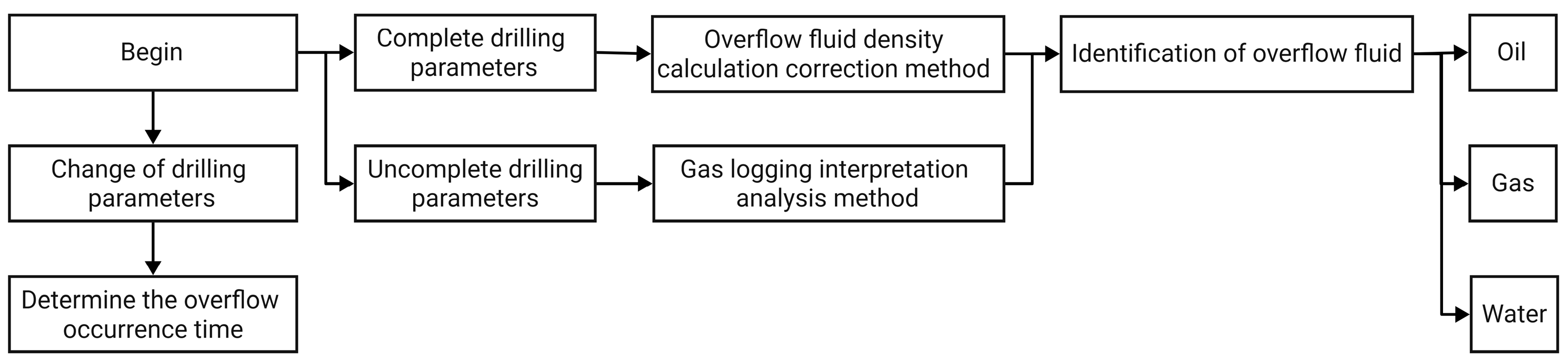
3.3. Identification Process of Overflow Fluid Type

As shown in Figure 6, the identification process of the overflow fluid proposed in this paper is as follows:

(1)

Determine the overflow occurrence time according to the change in drilling parameters;

(2)

If the drilling parameters during the overflow period are complete and normal without error, extract the drilling parameters during the overflow period, use the overflow fluid density calculation correction method to obtain the overflow fluid density, and identify the type of overflow fluid according to Table 1;

(3)

If there are no real-time drilling parameters or if the drilling parameters are abnormal, extract the gas logging at the time of the overflow and use the comprehensive analysis method of gas logging data to identify the type of overflow fluid;

(4)

If both drilling parameters and gas logging data can be used, compare the results obtained by the two methods and combine them with the field analysis to obtain the final identification result.

Figure 6. The process of identifying overflow fluid type.

Figure 6. The process of identifying overflow fluid type.

4. Example Calculation and Validation

4.1. OnSite Example Calculation

More than 20 overflow wells onsite were selected as examples to verify the accuracy of the identification methods for the overflow fluid. The reservoir in this area is highly heterogeneous, being ultra-deep, and having an ultra-high temperature and high pressure, with acid gas, and a complex leakage and overflow, which makes the risk of drilling high [25]. Therefore, it is necessary to identify the overflow fluid type.

Well Y uses water-based drilling fluid; the drilling parameters are shown in

Table 5. Identification results of overflow fluid types.

Well Name	Well Depth	Shut-In Standpipe Pressure	Shut-In Casing Pressure	Overflow Volume	ρmud	ρi	Identification Result	Test Result
Y	8547.72	5.04	5.82	0.6	1.29	0.29	Gas	Gas

. Combined with the change in drilling parameters, the overflow time was determined to be roughly 20 min.

Substitute the collected data, such as shut-in standpipe pressure, shut-in casing pressure, overflow volume, temperature, and pressure field data into Equation (10) for an iterative calculation; it can be obtained that the overflow fluid density of Well Y is 0.29 cm³, less than 0.36 cm³. According to Table 1, this can preliminarily identify the overflow fluid as gas. Table 5 shows the results of identifying Well Y.

The overflow volume and the overflow time were substituted into Equation (19) to calculate the average kick rate.

$$V_{\mathrm{k}}=\frac{S_{\mathrm{o}}}{T}$$

(20)

where $V_{\mathrm{k}}$ is the average kick rate, L/s; $S_{\mathrm{o}}$ is overflow volume, L; $T$ is overflow time, s.

The average kick rate was calculated to be 0.5 L/s. The wellbore structure, drilling assembly, and drilling parameters of Well Y were input into the two-phase flow model of the wellbore, and the gas rate in the shut-in annular space after the overflow gas kick in Well Y was obtained through the simulation calculation, as shown in Figure 7.

The collected drilling fluid data, drilling parameters, and calculated gas rate were substituted into Equation (15) for an iterative calculation, and the corrected density of the invaded fluid was 0.323 g/cm³. The corrected kicked fluid was identified to be gas, and the density was calculated more accurately than before the correction.

The gas logging data during the overflow period of Well Y was substituted into Equations (16)–(18) to calculate the 3H ratio of hydrocarbons, which were drawn in a 3H ratio diagram, as shown in Figure 8. According to the identification method, the overflow fluid in Well Y was judged to be recoverable gas. As shown in Table 4, the density range is 0.15 g/cm³–0.34 g/cm³, which is the same as that of the overflow fluid density calculation correction method, and in line with the subsequent test result.

The method proposed in this study was used to identify the overflow fluid type in 20 overflow wells onsite. Of these wells, the identification results of two wells were inconsistent with the later test results due to abnormal drilling parameters. The identification of the rest of the wells was consistent with the later test results. It was proven that the method is effective, with an accuracy rate of more than 90%, with strong practicability and suitability for different drilling sites, and has guiding significance for onsite overflow treatment and any subsequent research.

4.2. Validation of Overflow Fluid Density Model

Since the downhole overflow fluid density cannot be measured, this study used the real gas equation to calculate the density and verify the accuracy of the overflow fluid density correction method proposed in this study, selecting Well C as an example [9,26]. The real gas deviation factor can be calculated by the equations as follows:

$$Z=A+\frac{1-A}{e^B}+(0.132-0.32\lg T)P^C$$

(21)

$$A=1.39{(T-0.92)}^{0.5}-0.36T-0.101$$

(22)

$$B=(0.62-0.23T)P+(\frac{0.066}{T-0.86}-0.037)P^2$$

(23)

$$\rho ={\displaystyle \sum _{i=1}^n{\rho }_{gi}{f}_i}$$

(24)

The formation fluid density on the ground can be calculated by Equation (24).

$$C={10}^{0.3106-0.49T+0.1824T^2}$$

(25)

The volume ratio between the surface and the bottom hole can be calculated by the real gas equation:

$$V_{\mathrm{b}}=\frac{T_{\mathrm{b}}{P}_{\mathrm{s}}}{T_{\mathrm{s}}{P}_{\mathrm{b}}}{V}_{\mathrm{s}}$$

(26)

In these equations, ${\rho }_{gi}$ is the ground density of the gas component i, g/cm³; $f_i$ is the Moore score of gas component i, %; $V_{\mathrm{b}}$ is the gas volume under the bottom of the well, m³; $V_{\mathrm{s}}$ is the gas volume under the ground condition, m³; $T_{\mathrm{b}}$ is bottom hole temperature, °C; $T_{\mathrm{s}}$ is ground temperature, °C; $P_{\mathrm{b}}$ is bottom hole pressure, MPa; $P_{\mathrm{s}}$ is ground pressure, MPa.

The gas composition of the overflow formation in Well C is shown in Figure 9.

The fluid density can be calculated by the above equations and the gas composition with the formation fluid analysis. The calculation results of Well C are shown in

Table 6. The calculation results of Well C.

Traditional Method Density (g/cm3)	Correction Method Density (g/cm3)	Overflow Fluid Density (g/cm3)
0.282	0.269	0.272

.

The calculation result of the traditional method is 0.01 and the relative error is 3.7%. The error of the calculation result of the correction method is 0.003 and the relative error is 1.11%. The overflow fluid density calculated by the overflow fluid density correction method proposed in this study has a higher accuracy than the traditional method.

5. Analysis of Influencing Factors for Overflow Fluid Density

(1)

The geothermal gradient

The density of drilling fluid varies with the geothermal gradient. Figure 10 shows the change curve of the overflow fluid density with different geothermal gradients.

As can be seen from Figure 10, as the geothermal gradient increases, the density of overflow fluid shows a downward trend. When the geothermal gradient is 1.5 °C/100 m, the overflow fluid density is 0.274 g/cm³, while when the geothermal gradient rises to 3 °C/100 m, the overflow fluid density decreases to 0.264 g/cm³, for a total decrease of 0.01 g/cm³.

(2)

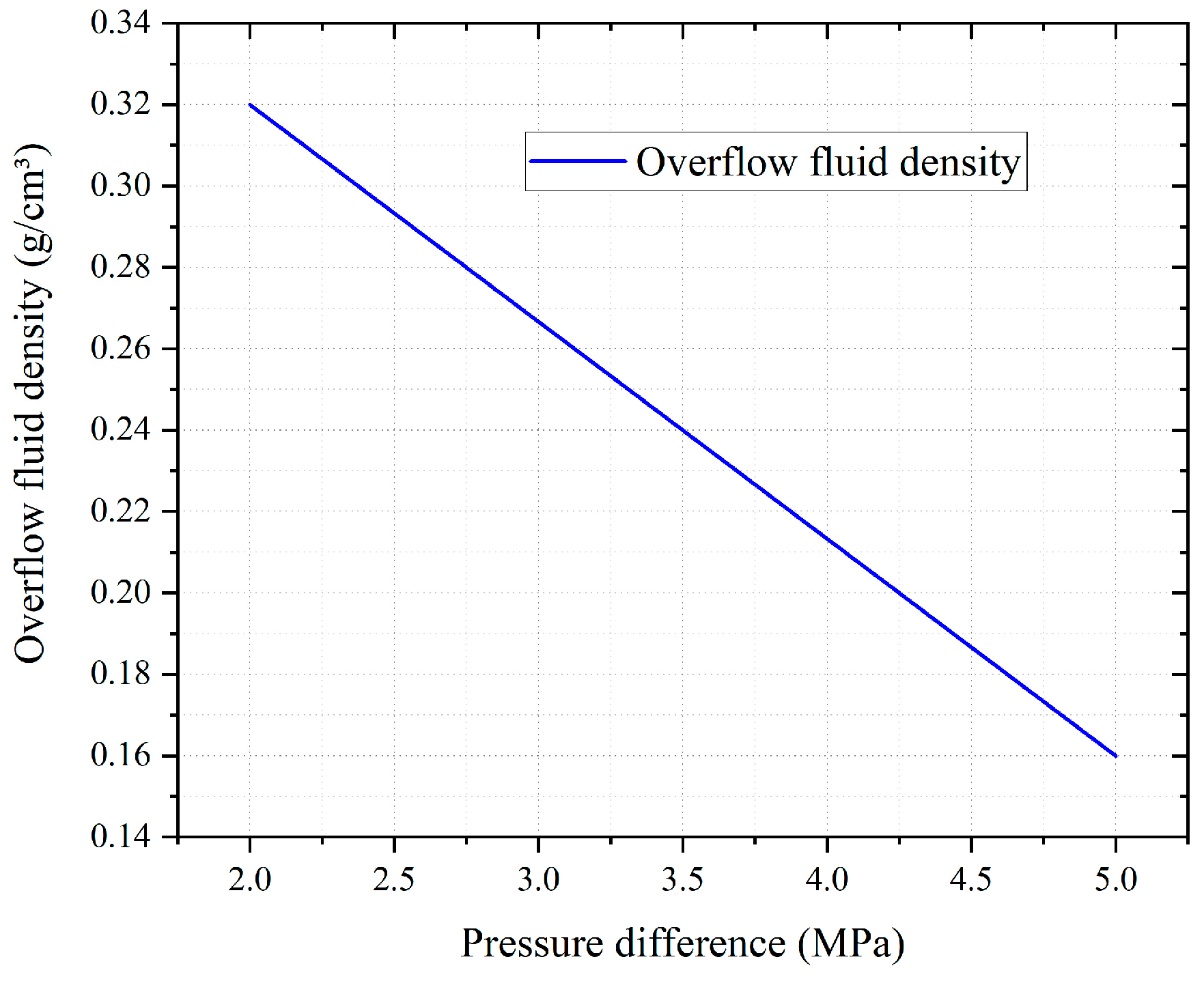
The pressure difference between standpipe pressure and casing pressure

The pressure difference between standpipe pressure and casing pressure directly reflects the magnitude of the overflow fluid density, which has a negative relationship with the overflow fluid density. When the kick amount is unchanged, an increase in the pressure difference causes the overflow fluid density to gradually decrease.

As can be seen from Figure 11, the overflow fluid density is 0.32 g/cm³ when the pressure difference is 2 MPa; when the pressure difference rises to 5 MPa, the overflow fluid density is 0.16 g/cm³.

(3)

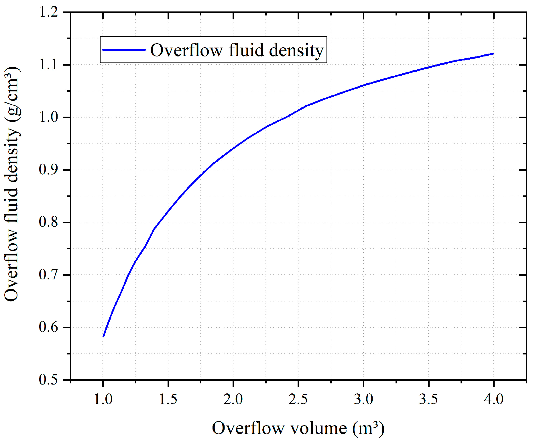
The amount of overflow fluid

When the amount of overflow fluid increases and the other conditions remain unchanged, the length of the mixed drilling fluid in the wellbore increases, but the pressure of the liquid column decreases by the same amount, so the density of the intruding fluid will gradually increase as the amount of the overflow fluid increases.

As is shown in Figure 12, an increase in the amount of overflow fluid results in the growth rate of the overflow fluid density gradually slowing down. The overflow fluid density is 0.58 g/cm³ when the amount of overflow fluid is 1 m³, while when the influx of overflow fluid is 4 m³, the overflow fluid density rises to 1.12 g/cm³.

6. Summary and Conclusions

(1)

In this paper, a comprehensive multi-factor method for identifying the types of overflow fluid is established, which includes a comprehensive analysis of the method of gas logging and the method of the correction of the overflow fluid density calculation. When comparing this method with field test results from more than 20 overflow wells onsite, the discriminant accuracy of this method was over 90% and the density calculation accuracy was higher than that of the traditional model.

(2)

In this paper, the effects of geothermal gradient, vertical casing pressure difference after well shut-in, and formation fluid kick-on of the overflow fluid density were analyzed. It was found that as the geothermal gradient increases, the overflow fluid density decreases; when the kick amount is constant, an increase in the pressure difference gradually decreases the overflow fluid density. When other conditions remain unchanged, the kick amount increases, and the growth rate of overflow fluid density gradually slows down.

(3)

The comprehensive method presented in this paper can be used to provide guidance for handling overflow accidents in the field and ensure that drilling operations are carried out safely.

(4)

In further research based on this paper, the density model can be improved by considering different working conditions, and a new gas logging analysis method with greater accuracy may be proposed.

References

- Li, Y.; Xue, Z.; Cheng, Z.; Jiang, H.; Wang, R. Progress and Development directions of deep oil and gas exploration and development in China. China Pet. Explor. 2020, 25, 45–57. [Google Scholar]
- Zhang, G.; Ma, F.; Liang, Y.; Zhao, J.; Qin, Y.; Liu, X.; Zhang, K.; Ke, W. Domain and theory-technology progress of global deep oil & gas exploration. Acta Pet. Sin. 2015, 36, 1156–1166. [Google Scholar]
- Guan, Z.; Chen, T. Drilling Engineering Theory and Technology; Petroleum University Press: Beijing, China, 2000. [Google Scholar]
- Compilation of Blowout Accident Cases of China National Petroleum Corporation; Petroleum Industry Press: Beijing, China, 2006.
- Wang, P.; Luo, P.; Nie, X.; Zhang, X.; Yang, L. Treatment of complicated well conditions with blowout and leakage in Well Shuangmiao 1. Nat. Gas Ind. 2007, 27, 4. [Google Scholar]
- Zhang, G. Analysis of Overflow Killing in Well Qingxi 1. Pet. Drill. Tech. 2009, 37, 5. [Google Scholar]
- Zhang, G. Oil Drilling Technology about One-cycle Killing Technology from Typical Blowout Cases. Pet. Drill. Tech. 2018, 46, 6. [Google Scholar]
- Bi, W. On-Site Killing Method Optimization and Well Killing Process Simulation Research; China University of Petroleum: Beijing, China, 2006. [Google Scholar]
- Drilling Manual; Petroleum Industry Press: Beijing, China, 1990.
- Li, J.; Lei, J.; Hou, X. Discussion about the application of comprehensive interpretation method of gas logging in Tarim Basin. Logging Eng. 2003, 14, 18–24. [Google Scholar]
- Huang, X. Gas logging and logging methane correction method and gas logging interpretation method selection principle. Logging Eng. 2007, 18, 1–5. [Google Scholar]
- Hou, P. A method for comprehensively discriminating oil and gas water layers using logging data. Logging Eng. 2008, 19, 1–8. [Google Scholar]
- Hou, P. A simple parameter method of gas logging to identify oil, gas and water layers. Logging Eng. 2009, 20, 21–24. [Google Scholar]
- Duan, Y.; Zhang, J. Application of Light Hydrocarbon Triangle Method in Oil and Gas Reservoir Evaluation in Mahuangshan Area. Pet. Geol. Eng. 2010, 24, 43–46. [Google Scholar]
- Yu, M.; Bian, H.; Zhuang, W.; Zhu, D.; Ye, X.; Xue, Z. Analysis of applicability of Pixler chart interpretation method for gas logging. Logging Eng. 2013, 24, 14–19, 85–86. [Google Scholar]
- Li, Z.; Hu, W.; Xia, Y.; Chen, X.; Wei, F. Studies about the method for identification of the oil gas layer types with gas logging data. Offshore Oil 2015, 35, 78–85. [Google Scholar]
- Su, Y.; Lu, B.; Liu, Y.; Zhou, Y.; Liu, X.; Liu, W.; Zang, Y. Status and research suggestions on the drilling and completion technologies for onshore deep and ultra-deep wells in China. Oil Drill. Prod. Technol. 2020, 42, 527–542. [Google Scholar]
- Wang, Z.; Hao, X.; Wang, X.; Xue, L.; Guo, X. Numerical Simulation on Deepwater Drilling Wellbore Temperature and Pressure Distribution. Pet. Sci. Technol. 2010, 28, 911–919. [Google Scholar] [CrossRef]
- Wu, Z.; Xu, J.; Wang, X. Predicting temperature and pressure in high-temperature–high-pressure gas wells. Petrol. Sci. Technol. 2011, 2, 132–148. [Google Scholar] [CrossRef]
- Yan, J.; Li, Y. Mathematical model for predicting mud density at high temperature and pressure. Oil Drill. Prod. Technol. 1990, 12, 27–34. [Google Scholar]
- Wang, E.; Fan, H.; Ma, L. Simple method for calculating the down-hole drilling fluid density. Sci. Technol. Rev. 2015, 33, 54–58. [Google Scholar] [CrossRef]
- Fan, H. Practical Drilling Fluid Mechanics; Petroleum Industry Press: Beijing, China, 2014. [Google Scholar]
- Chen, J. Petroleum Gas-Liquid Two-Phase Pipe Flow; Petroleum Industry Press: Beijing, China, 1989. [Google Scholar]
- He, H.; Tong, J.; An, Y. Research on triangle illustration to gas logging hydrocarbon component. J. Tianjin Inst. Technol. 2004, 20, 30–33. [Google Scholar]
- Zhou, B. Research on Complex Process Treatment Technology under MPD Conditions in Tazhong Area; China University of Petroleum: Beijing, China, 2017. [Google Scholar]
- Hu, J. A new method to calculate the Z factor of natural gases. Acta Pet. Sin. 2011, 32, 862–865. [Google Scholar]