Reliable Tools to Forecast Sludge Settling Behavior: Empirical Modeling

Abstract

In water- and wastewater-treatment processes, knowledge of sludge settlement behavior is a key requirement for proper design of a continuous clarifier or thickener. One of the most robust and practical tests to acquire information about rate of sedimentation is through execution of batch settling tests. In lieu of conducting a series of settling tests for various initial concentrations, it is promising and advantageous to develop simple predictive models to estimate the sludge settlement behavior for a wide range of operating conditions. These predictive mathematical model(s) also enhance the accuracy of outputs by eliminating measurement errors originated from graphical methods and visual observations. In the present study, two empirical models were proposed based on Vandermonde matrix (VM) characteristics as well as a Levenberg–Marquardt (LM) algorithm to predict temporal height of the supernatant–sludge interface. The novelty of our modeling approach is twofold: the proposed models in this study are more robust and simpler compared to other models in the literature, and the initial sludge concentration was considered as a key independent variable in addition to the more-customarily used settling time. The prediction performance of the VM-based model was better than the LM-based model considering the statistical parameters associated with the fitting of the experimental data including coefficient of determination (R²), root mean square error (RMSE), and mean absolute percentage error (MAPE). The values of R², RMSE, and MAPE for the VM- and LM-based models were obtained at 0.997, 0.132, and 5.413% as well as 0.969, 0.107, and 6.433%, respectively. The proposed predictive models will be useful for determination of the sedimentation behavior at pilot- or industrial-scale applications of water treatment, when the experimental methods are not feasible, time is limited, or adequate laboratory infrastructure is not available.

1. Introduction

Different physical, chemical, and biological processes are used to remove contaminants from water and wastewater [1,2]. As shown in Figure 1, in a conventional wastewater-treatment plant, the first stage is primary treatment, which focuses on removing large suspended solids through a physical separation process such as screening and gravity settling. The next stage is secondary treatment or biological treatment, and the last stage is tertiary treatment, where the treated water is chemically polished and disinfected if necessary [3]. The sedimentation process is one of the key mechanisms commonly used after secondary treatment or chemical addition to separate suspended particles. One of the most common methods for physical separation of solid particles from water or wastewater, the so-called clarification stage, is an effective gravity sedimentation process through which the underflow solids are being concentrated for recycling or disposal purposes (aka thickening process) [3]. The gravity sedimentation process can be assessed in lab- or pilot-scales through simple yet time-consuming experimental methodologies; therefore, efforts have been made to propose mathematical models as a practical alternative for assessment of the sedimentation process performance as well as optimization of the design and operation of the industrial sedimentation units. Various processes have taken advantage of the settling process such as removal of impurities, color, and turbidity by coagulation and flocculation, water softening by chemical precipitation, removal of 50–70% of the suspended solids, and containment of 25–40% of the Biological Oxygen Demand (BOD) from the municipal wastewater by primary treatment followed by removal of biological flocculent mass produced by microorganisms through secondary treatment [3]. Other applications of the settling process include removal of grit in the preliminary stage as well as separation of the digested sludge from the supernatant liquor within the secondary sludge digesters (see Figure 1) [3]. Sludge thickeners are also widely used in the water- and wastewater-treatment processes to reduce the volume of sludge before pumping it into the drying beds, a filter press, belt press, or other applications [3]. The unit area of a well-designed thickener is obtained through calculations based on the settling curves.

The foundation of sedimentation modeling was based on the classical Kynch theory of sedimentation, in which the sedimentation velocity was solely a function of the local particle concentration [4]. On the basis of this assumption and the law of mass conservation, a first-order nonlinear partial differential equation (PDE) was suggested as the governing equation for the batch settling process. Solving the proposed particle settling governing equation has always been a challenging task. For instance, Kynch developed a solution for this PDE by assuming wave propagation of equal concentration layers in an ideal batch settling process (i.e., with no compression). This so-called characteristic analysis approach is the only available analytical solution for the proposed particle settling governing equation; however, it has been reported problematic for implementation [5,6]. To ease analytical model implementation, some numerical solution methodologies using numerical flux concepts were developed [7]. Some early efforts were also dedicated to accounting for more-realistic factors in the sedimentation process (and its governing equation) such as dispersion and compression of the settled bed [8]. Bürger et al. [9] included both compression at high concentrations and dispersion due to turbulence through separate functions in the governing PDE. Bürger et al. [10] presented a solution methodology for this model using spatial discretization or time discretization of the governing PDE, resulting in developing a set of ordinary differential equations (ODEs) which were then solved by numerical simulation in conjunction with ODE solvers (i.e., method-of-line formulation) [11]. Using this method, more-realistic simulation of secondary sedimentation tanks was performed under unusual climate conditions such as wet weather [12].

Most of the well-known sizing studies utilize the solid mass flux method to determine the required area of continuous sedimentation systems [13,14,15,16]. One of the widely used methods to produce the solid mass flux curve takes advantage of Kynch’s method for extraction of some parameters such as settling velocity and local concentrations to estimate a significant portion of the flux function with only one batch settling test. Diehl used this method for the greatest solid concentrations and suggested a new batch settling test from which the flux function was theoretically estimated for the smaller solid concentrations [17]. For these two solid concentration regions, some general explicit formulae were derived. Considering both these methods for solid mass flux determination in a typical sedimentation process, the height variations associated with the solid–liquid interface should be properly characterized.

In addition to the two methods described above, some empirical velocity functions are repeatedly used in the literature in order to determine the solid mass flux curves in which the sedimentation velocity is determined using a regression method with the knowledge of initial solid concentration and maximum sedimentation velocity [16,18,19]. There are also theoretical approaches that have been developed based on mass and momentum conservation law such as the Vesilind model as well as the Cho model [18,20]. In a comparative study, Vanderhasselt and Vanrolleghem fitted various velocity models to a single batch settling curve and concluded that the Vesilind model was superior to the Cho model in describing the settling velocity. However, when the dynamics of the sludge blanket descent were fast, the Vesilind model failed but the Cho model was successful in describing the complete settling curves [21]. Various factors have been used to characterize the settling velocity including solid particle size, shape, sludge viscosity, density, and porosity; however, in practical engineering applications, empirical functions are preferred due to their simplicity and practicality [7].

One of the indispensable pieces of information for constructing settling flux functions is the variation of the supernatant–suspension interface height with time, extracted from the batch settling tests. Despite being simple and direct, the standard jar test used for measuring sedimentation rates suffers from some issues such as possible misinterpretation or subjective reading of the interface [22]. Other drawbacks include the monotonous and tedious nature of manual interface tracking, especially for long settling durations or when a flocculent (or coagulant) solution is added at greater dosage values and in a short time [23]. In response to all these issues and to minimize the test time, various methods have been proposed in the literature for determining the suspension settling characteristics and detecting the phase separation boundary, including the electrical capacitance [24] or conductance method [25], ultrasonic methods [26], γ-ray radiation [27], light sensors [28,29,30], numerical methods [31], hydrostatic pressure measurement [32], magnetic resonance imaging [33], or CCD video analysis [22,34,35]. One major downside associated with these state-of-the-art methods is the involvement of specialized high-tech equipment, which makes them expensive or time-consuming [22].

For flux identification and sedimentation characterization purposes, various studies have been carried out in order to determine explicit expressions for solid mass flux function. For instance, Zheng and Bagley presented a numerical procedure to simultaneously solve the momentum balance equation and 1-D continuity equation in a batch solid settling process, which resulted in determination of interface height variations as well as vertical solid profile versus time [36]. In another study, Wu and Chern presented a wave approach to predict the batch settling curves of heavy metal sludge over a long period of time [37]. The authors first employed the Vesilind model to determine the settling parameters for shorter time durations, and subsequently applied Kynch sedimentation theory as well as wave propagation theory to describe the whole settling curve. Grassia et al. [38] used a settling flux function proposed by Lester et al. [39] to generate an interface height profile for a synthetic batch settling process, and concluded that the interface height variations by time were reasonably fit with power law and exponential decay functions. The authors also explicitly correlated the settling flux function with the parameters associated with the power law fitting curves. In a subsequent study on the batch settling process, Grassia et al. [40] proposed a local fitting procedure instead of the global fitting approach in order to determine the interface height variations with time. The authors fitted the settling flux data with particular function(s) over small solid fraction intervals, and adjusted the function parameters to achieve a close match between the measured and predicted interface height values. By modifying the classical Kynch’s theory, van Deventer et al. [41] developed a semi-analytical method that incorporates the effect of aggregate densification (i.e., expelling liquid phase) by shear on settling properties. Using this analytical approach, the authors constructed the slurry–liquid interface height profile versus time, and compared the estimated values with some experimental data as well as numerical simulation results for a sheared batch settling process. Betancourt et al. [42] utilized the Kynch test and Diehl test to measure the suspension–supernatant interface height versus time, each representing the convex and concave segments of the flux curve, respectively [42]. They approximated the interface height by three functional forms so that the convexity or concavity condition was satisfied for all test data. Finally, using these functions, the researchers obtained the convex and concave parts of the flux curve using the Bürger–Diehl approach [10]. Zhang et al. [19] extended the theory developed by van Deventer [43] to devise an initially networked batch settler in which the suspension gel resists compression up to the compressive yield stress, resulting in formation of very slow aggregate densification. Li and Stenstrom [6] explained how the characteristics method can be developed in order to analytically solve the ideal continuous settling. The authors predicted the recycle concentration as well as the interface change as a function of time under different loading conditions using an analytical and three numerical approaches [6].

According to the above review of the available literature, two main methods are involved in the estimation of the solid flux curves: graphical and numerical simulation methods. The graphical flux estimation method involves visual tracking of the interface, which makes it prone to errors. It is also time-consuming to execute a series of settling tests at various initial solid concentrations. As an alternative for this tedious experimental methodology, the numerical simulation method is utilized as a predictive tool based on the application of correlations. Both these procedures depend on the variations of the supernatant–slurry interface height with time as well as the initial solid concentration. When a correlation for the interface height at each time interval is available, the sedimentation velocity can be calculated through differentiation of the interface height correlation. Thereafter, the solid flux curve can be prepared in order to design the thickener unit [44]. A review of the literature shows that very limited research work has been dedicated to the approximation of interface variation with time using curve fitting [38,44,45,46]. The prediction accuracy of the solid flux function significantly depends on the extent to which the experimental sedimentation data are approximated using the curve fitting procedure. Grassia et al. [38] assessed some plausible functional forms to simulate the batch settling data (i.e., interface height versus time), and reported that the quadratics fitting functions produced satisfactory results, whereas the power law and exponential decay fitting functions resulted in better predictions [38]. Banisi and Yahyaei [44] proposed a model, with several fitting parameters, to fit solid settling curves; however, its applicability seems problematic due to the large number of tuning parameters. Zhang et al. [45] used a logistic functional form to match the settling height versus time for batch settling tests. In addition, Kang et al. [46] proposed an S-shaped model based on the analysis of the form associated with the typical sedimentation curves. Both methods by Zhang et al. [19] and Kang et al. [46] resulted in satisfactory match of the experimental data for the batch sedimentation tests.

Due to the absence of more-efficient modeling approaches in the literature for predicting solid settling behavior, the main objective of this study was to develop more-representative yet simpler predictive models to capture the true physics of the solid settling phenomenon. In all the previous modeling attempts, the only independent parameter affecting the interface height was the settling time. We believe that the sedimentation process is a complex phenomenon, and that more independent parameters should be considered when predicting solid settling flux. For instance, initial solid content of the mixture significantly affects the settling phenomenon. Therefore, we aimed to develop correlations between the supernatant–sludge interface height (as the dependent variable) and the settling time as well as initial solid content, the two independent parameters, to help designing industrial thickeners or clarifier units. Two empirical correlations were used to model the sludge settlement process. These two correlations, solely in algebraic form, that do not rely on the graphic plots of sedimentation behavior hence possess greater prediction accuracy. The utilized correlations are simple, incorporate both time and initial solid concentrations as independent parameters, and contain a few tuning parameters which could be adjusted using limited experimental data. The first model was developed based on the Vandermonde matrix, and its coefficients were obtained using the matrix method. The coefficients of the second empirical model were optimized using the Levenberg–Marquardt algorithm, which resulted in minimization of the errors associated with the estimated batch sludge settling curves. The present work covers some novel aspects that have not been considered before in the literature: both the settling time and initial solid concentration were considered as the influencing parameters for predicting solid settling behavior (i.e., the greater the initial solid concentration, the longer it takes to settle), and the proposed simple correlations have been introduced for the first time to simulate the batch sedimentation behavior.

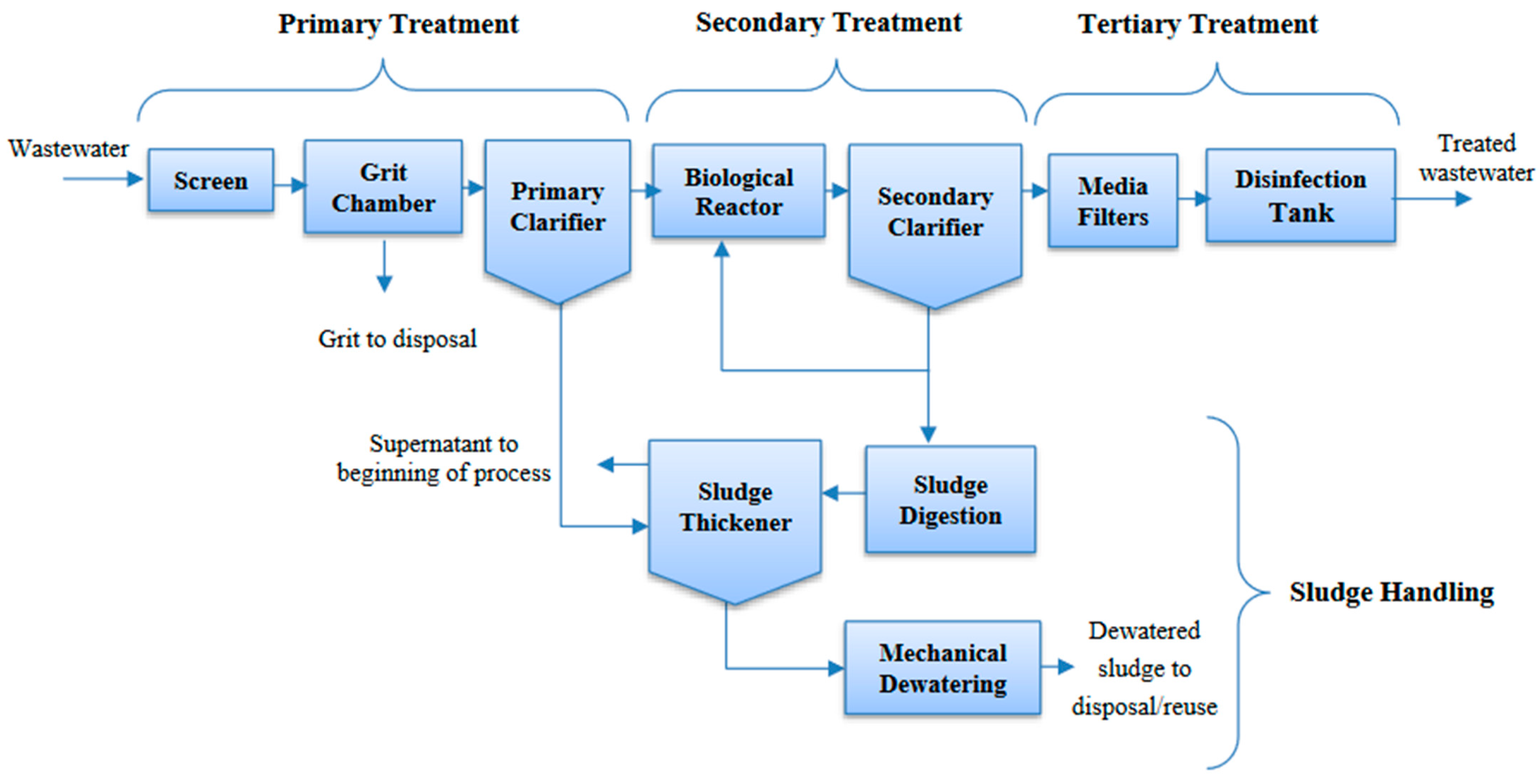
2. Description of the Sedimentation Process

Sedimentation is a physical process through which solid particles, with greater density values compared to the surrounding liquid phase, separate due to the gravity effect. In a tank with very slow suspension intake velocity, the solid particles tend to migrate toward the bottom due to gravity segregation. The supernatant phase in the sedimentation tank becomes clear while the particles accumulated at the bottom form a sludge layer. The sedimentation unit is one of the most important sections in a conventional wastewater-treatment system [47]. The main advantages of a sedimentation unit are cost effectiveness and low energy consumption (i.e., it only uses earth’s gravity force as the driving energy). The main disadvantage of the sedimentation unit is long separation time as well as large land area footprint [48]. A schematic flow diagram associated with a conventional wastewater treatment is illustrated in Figure 1.

The main steps of a wastewater-treatment plant include combination of primary treatment, secondary treatment, and tertiary or final treatment [3]. First, the coarser contaminants are separated by a screen, and then the grit and settleable solids are separated in two stages by gravity sedimentation (in a grit chamber and primary clarifier). After that, the digestible pollutants are consumed by microorganisms in the activated sludge process, and the treated effluent is separated from the remaining biomass in the secondary clarifier before entering the filtering and disinfection stages. In some industrial units, a chemical treatment step and a sedimentation process are also applied before filtration. The sludge obtained from the secondary sedimentation after biological digestion, along with the sludge obtained from the primary clarifier, enter the sludge thickener. Before the mechanical dewatering stage, the water content and sludge volume are reduced by sedimentation [3].

Therefore, the main applications of a sedimentation unit in wastewater treatment are [47]:

-

Preliminary treatment: Grit removal (i.e., sedimentation of inorganic particles of large dimensions);

-

Primary sedimentation: Sedimentation of suspended solids from the raw sewage;

-

Secondary treatment: Secondary sedimentation (i.e., removal of mainly biological solids);

-

Sludge treatment: Thickening (i.e., settling and thickening of primary sludge and/or excess biological sludge), and;

-

Physical–chemical treatment: Solid particle settling after chemical-induced precipitation.

The efficiency of a sedimentation unit is defined as its effectiveness in removing various constituents from water or wastewater. In wastewater treatment, the efficiency of the sedimentation unit is affected by various parameters such as type of the solids dispersed in the wastewater, temperature, and age of the solids [49]. Most of the conventional wastewater-treatment plants use activated sludge and are operated under ambient temperature [50].

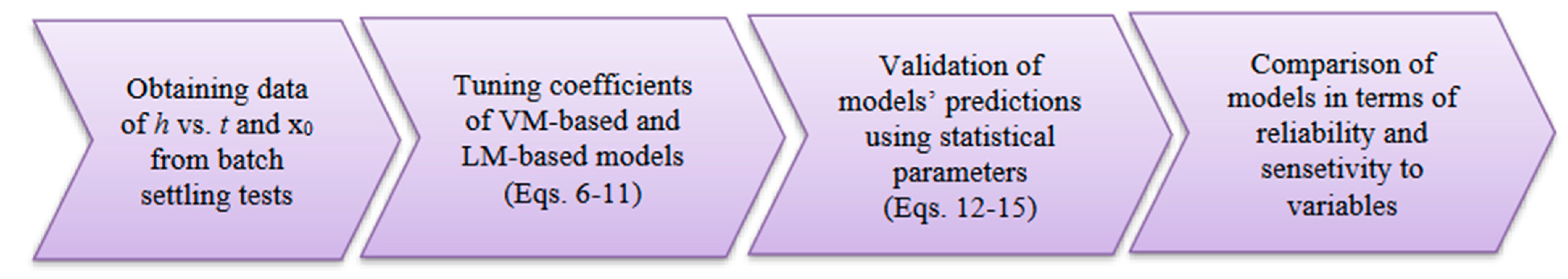
3. Materials and Methods

In order to develop correlations between the supernatant–sludge interface height and time as well as initial sludge concentration, some experimental interface heights as a function of time and solid concentration are needed for tuning the model parameters. The experimental data were borrowed from the study by Vanderhasselt and Vanrolleghem [21]. According to the review of literature provided in Section 1, the solution to slurry–supernatant interface variations with time and initial solid content should be obtained by solving some governing partial differential equations [4]. The sediment flux functions should be constructed from the batch settling data. The available models for solid flux prediction are categorized into three groups: (1) expressions for the flux density function in terms of some parameters such as solid fraction and sedimentation velocity [17]; (2) sedimentation velocity models that are assumed to be only a function of the local solid concentration [18], and; (3) expressions for interface height as a function of the settling time [38]. The latter category, prediction of interface height change as a function of the settling time, is a fundamental step in constructing sedimentation flux functions from the batch sedimentation experiments. The sedimentation velocity is obtained from the slope of such a curve at each corresponding settling time. It is challenging to obtain a universal relationship that could predict the sedimentation velocity for the whole range of solid concentration. The accuracy of predictions greatly depends on the appropriateness of the curve fitting exercise, i.e., a poor curve fitting to match the trends associated with the interface height versus time and solid content will result in erroneous predictions associated with the solid flux functions. Among the available curve fitting models, the power law and exponential decay functions have been commonly used in the literature [38]; however, they are unable to represent multiple nonlinear properties of the sedimentation curves.

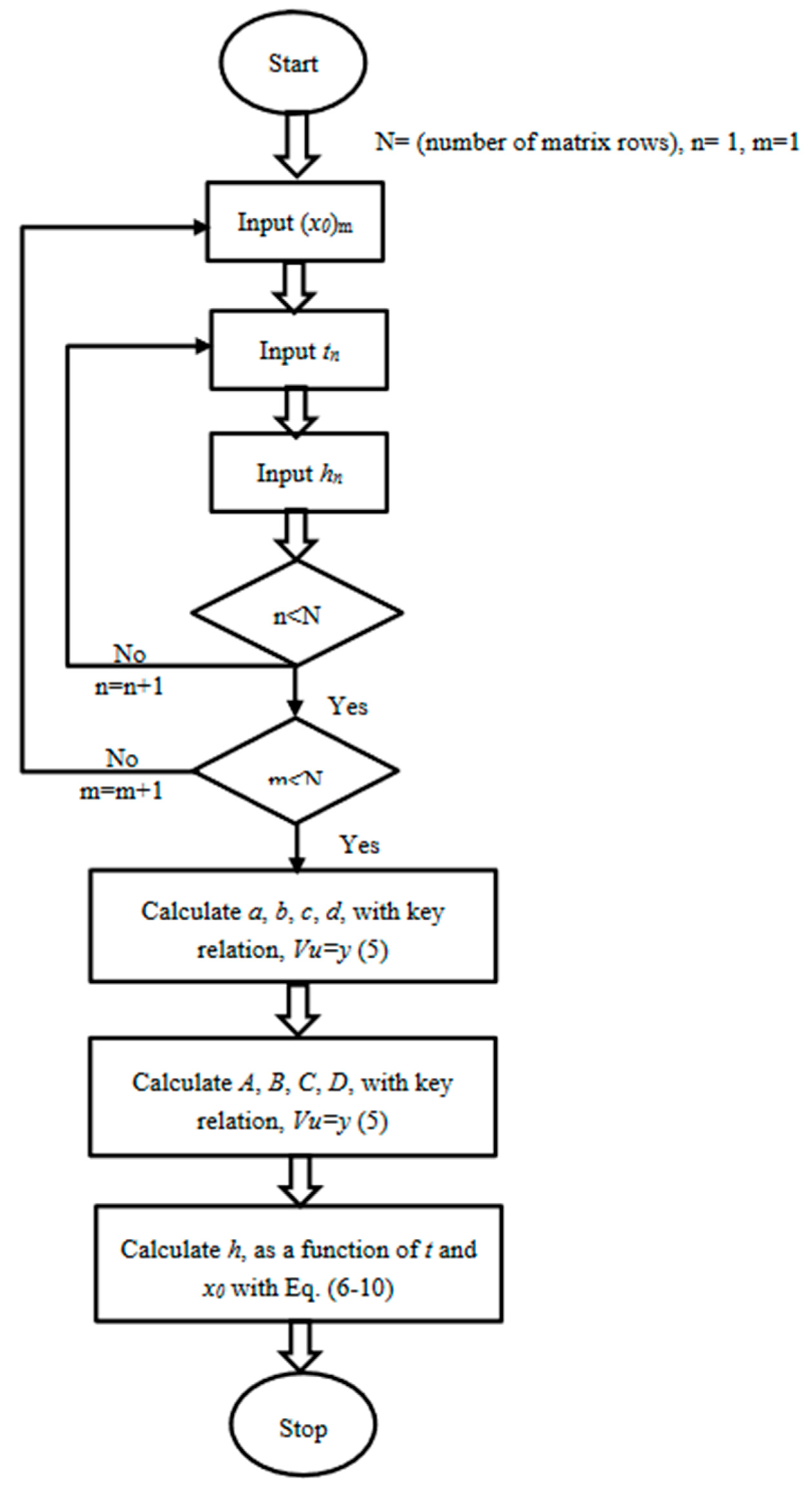
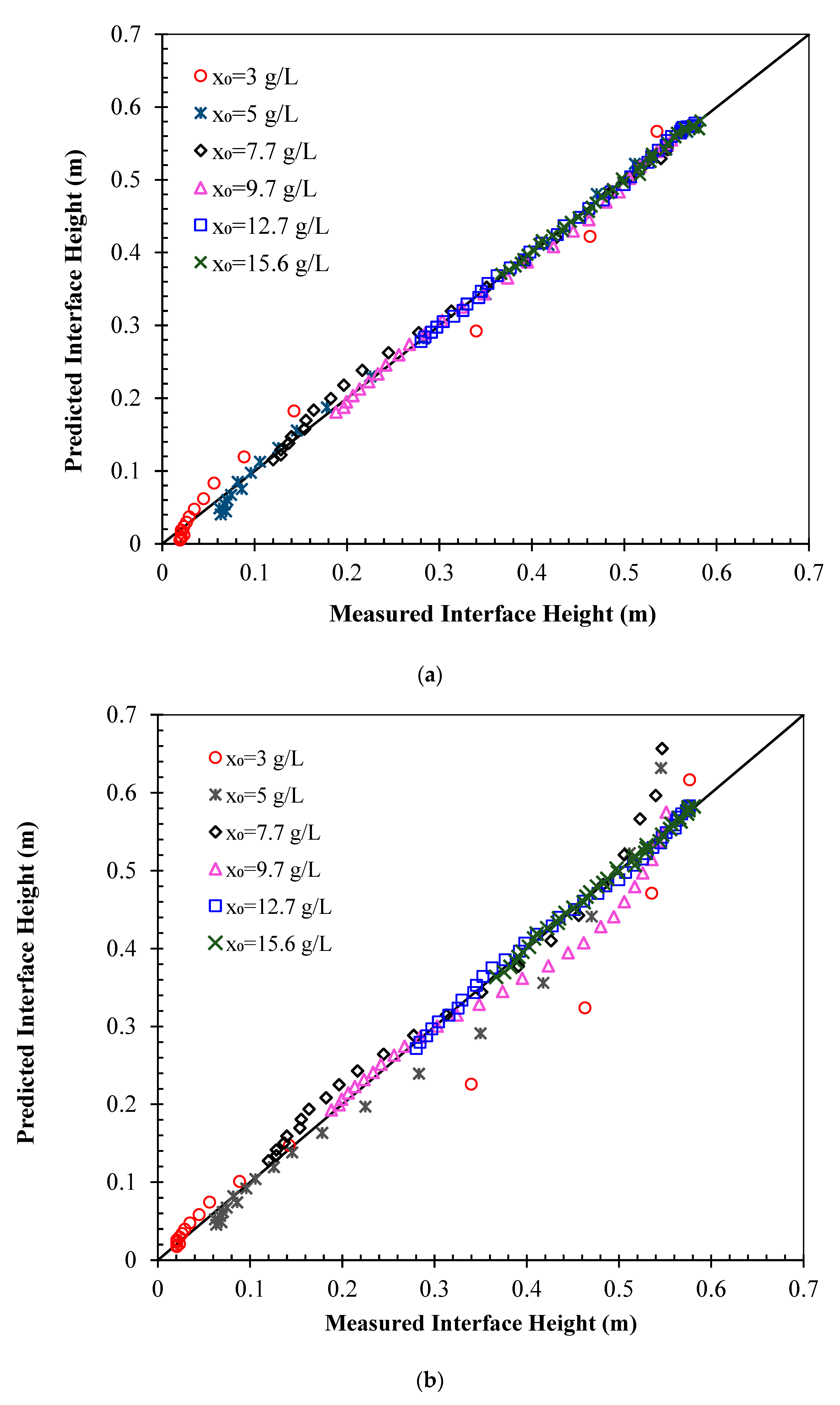
3.1. Correlation Based on the Vandermonde Matrix (VM)

The first model proposed in this paper is a correlation, developed based on the Vandermonde matrix (VM). The VM has a special form and appears in many applications such as mathematics, nuclear and quantum physics with direct implications in polynomial interpolation, least square regression, optimal experimental design, error-detecting and error-correcting, and discrete Fourier transformation calculations, along with some associated transformations such as fractional discrete Fourier transformation as well as quantum Fourier transformation [50,51]. Often, it is not the VM itself that is useful, but the multivariate polynomial given by its determinant (also known as the Vandermonde determinant, or Vandermonde polynomial, or Vandermondian), which is frequently utilized in many applications [50,52]. In the VM, a geometrical progression appears in each row, similar to the following equation for an m×n-1 matrix (m and n-1 are the number of rows and columns, respectively) [50,53]:

$$V=\left[\begin{array}{ccccc}1& x_1& x_1^2& \dots & x_1^{n-1}\\ 1& x_2& x_2^2& \dots & x_2^{n-1}\\ 1& x_3& x_3^2& \dots & x_3^{n-1}\\ ⋮ & ⋮ & ⋮& \ddots & ⋮\\ 1& x_m& x_m^2& \cdots & x_m^{n-1}\end{array}\right]$$

(1)

or

$$V_{i,j}=x_i^{j-1}$$

(2)

where V and x_i represent the Vandermonde matrix and elements of the matrix, respectively.

The determinant of the square VM (where m = n) can be calculated as [54,55,56]:

$$\det \left(V\right)={\displaystyle \prod }_{1\le i<j\le j<n}\left(x_j-x_i\right)$$

(3)

The VM can be used for polynomial interpolation between a set of points [54,55]. For instance, suppose a polynomial of degree n−1, f(x) is desired to pass through a set of n distinct points (x_i, y_i). This interpolation can be expressed mathematically as:

$$f\left(x\right)={\displaystyle \sum }_{j=0}^{n-1}{u}_j{x}^i$$

(4)

where u_j represents the unknown coefficients for the polynomial.

The non-vanishing of the Vandermonde determinant for distinct points x_i shows that the map from coefficients to values at those points is a one-to-one correspondence, and that the polynomial interpolation problem is solvable with a unique solution, the so-called unisolvence theorem [55,57]. Thus, it is useful in the polynomial interpolation since finding the unknown coefficients, a_j, from Equation (4) is equivalent to solving the following simple and linear equation [54,55]:

$$Vu = y$$

(5)

where u and y are the vectors of unknown coefficients and the corresponding values of y_i, respectively.

The VM can also be used to model multivariable functions. Equations (6)–(10) express the proposed correlations for estimation of the supernatant–sludge interface height as a function of time and initial solid content. Equation (6) directly correlates the interface height to the sedimentation time, while the rest of the equations determine implicit functionality between the interface height and the sludge concentration. This type of formulation has been used before in some studies in the literature to calculate heat flow as a function of the insulation thermal resistance and temperature drop, or to calculate the effluent and influent concentration ratio in a plug-flow reactor as a function of the dispersion factor, first-order reaction constant, and hydraulic detention time [54,55,56,57]:

$$h=a+b\times \frac{1}{t}+c\times \frac{1}{{\left(t\right)}^2}+d\times \frac{1}{{\left(t\right)}^3}$$

(6)

$$a=A_1+B_1\times x_0+C_1\times x_0{}^2+D_1\times x_0{}^2$$

(7)

$$b=A_2+B_2\times x_0+C_2\times x_0{}^2+D_2\times x_0{}^2$$

(8)

$$c=A_3+B_3\times x_0+C_3\times x_0{}^2+D_3\times x_0{}^2$$

(9)

$$d=A_4+B_4\times x_0+C_4\times x_0{}^2+D_4\times x_0{}^2$$

(10)

where h, t, and x₀ represent the interface height, sedimentation time, and initial solid concentration, respectively; a, b, c, d, A₁, A₂, A₃, B₁, B₂, B₃, C₁, C₂, C₃, D₁, D₂, and D₃ are fitting parameters which should be tuned using the experimental data.

Equations (6)–(10) are chosen to be of degree 3; hence, each of them has 4 coefficients. Therefore, 16 coefficients should be obtained for the complete description of this model. For tuning the model parameters, we collected the experimental data, including interface height variation with time and concentration, from a study conducted by Vanderhasselt and Vanrolleghem [21]. The solid settling experiments were conducted in the batch mode at room temperature, in a settling column of 70 cm height and 14 cm diameter, equipped with a 0.3 rpm stirrer. A settlometer was used to track and record the interface height variations after a dilution procedure was executed. In total, six settling curves for initial sludge concentrations ranging from 3 to 15.6 g/L were produced. According to Vanderhasselt’s observations, some early startup settling phenomenon occurred before the full descent blanket settling started; therefore, the settling velocity was multiplied by an on–off term which was 0 when the simulation time was smaller than the settling start time but was changed to 1.0 when the simulation time exceeded the settling start time [21]. In the present study, we shifted the modeling time to the actual instance when the sludge started to settle so that the interface height at time zero was the same as the initial sludge height. The stepwise implementation of the proposed methodology to find the optimal coefficients of the model is as follows:

(1)

At a given initial sludge concentration (x₀) and relevant height data (h), Equation (6) was applied and the coefficients a, b, c, and d were determined so that the interface height variations were correct function of the settling time using Equation (4).

(2)

The coefficients for Equation (6) were recalculated at each subsequent initial sludge concentration using step 1.

(3)

According to Equations (7)–(10), the coefficients A₁–A₃, B₁–B₃, C₁–C₃, and D₁–D₃ are dependent on the initial solid concentration. Therefore, these coefficients should be found so that the coefficients of the previous step in Equation (6), i.e., a, b, c, and d represent the correct functionality of the initial concentration. The different coefficients obtained from the previous steps (i.e., a, b, c, and d) were correlated to the initial concentration, and the new coefficients (i.e., A₁–A₃, B₁–B₃, C₁–C₃, and D₁–D₃) for Equations (7)–(10) were obtained in a similar way using Equation (4).

In Figure 2, a flowchart is presented that demonstrates the process through which the parameters associated with Equations (6)–(10) are tuned for parameter optimization.

3.2. Correlation Based on the Levenberg–Marquardt (LM) Algorithm

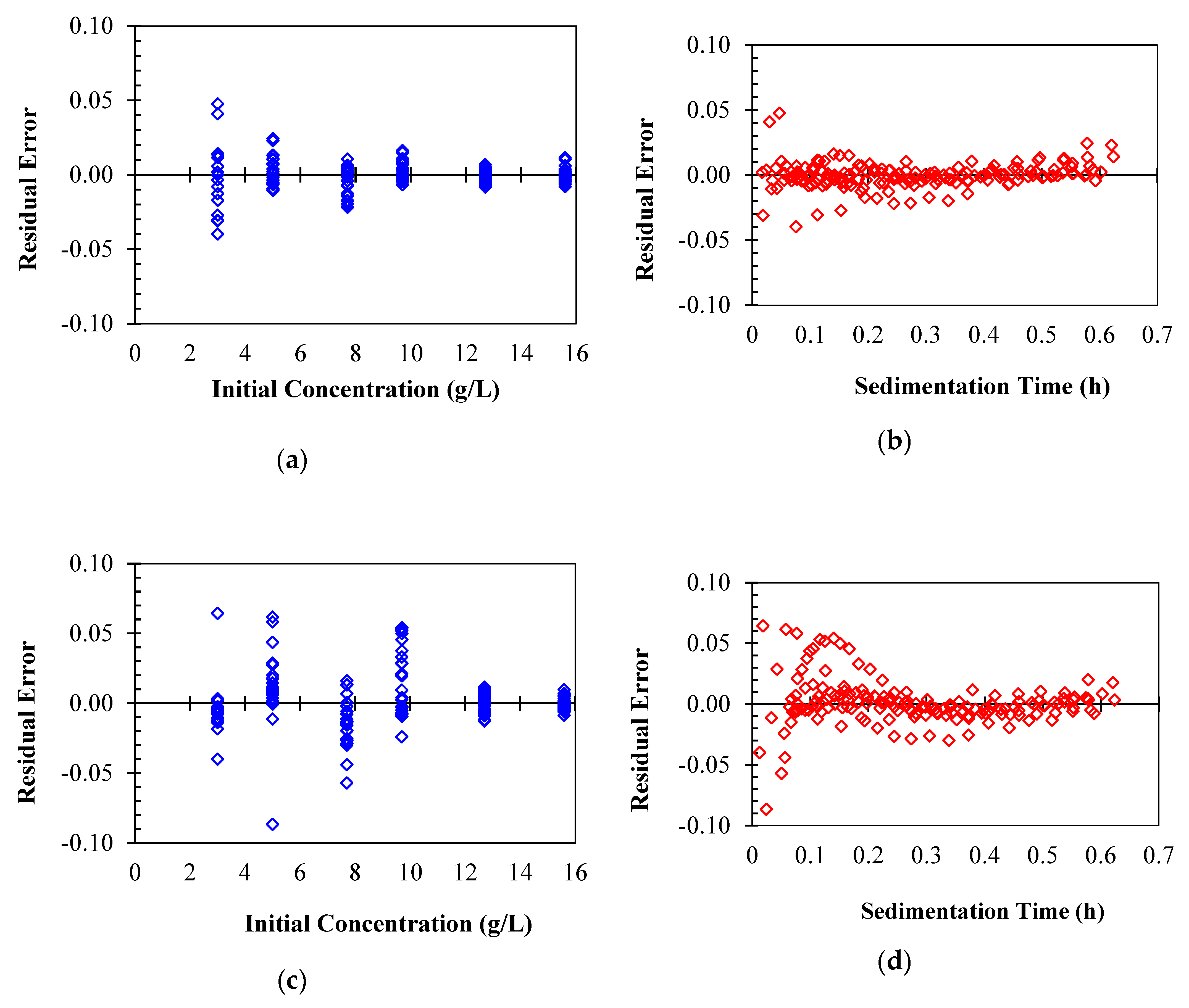
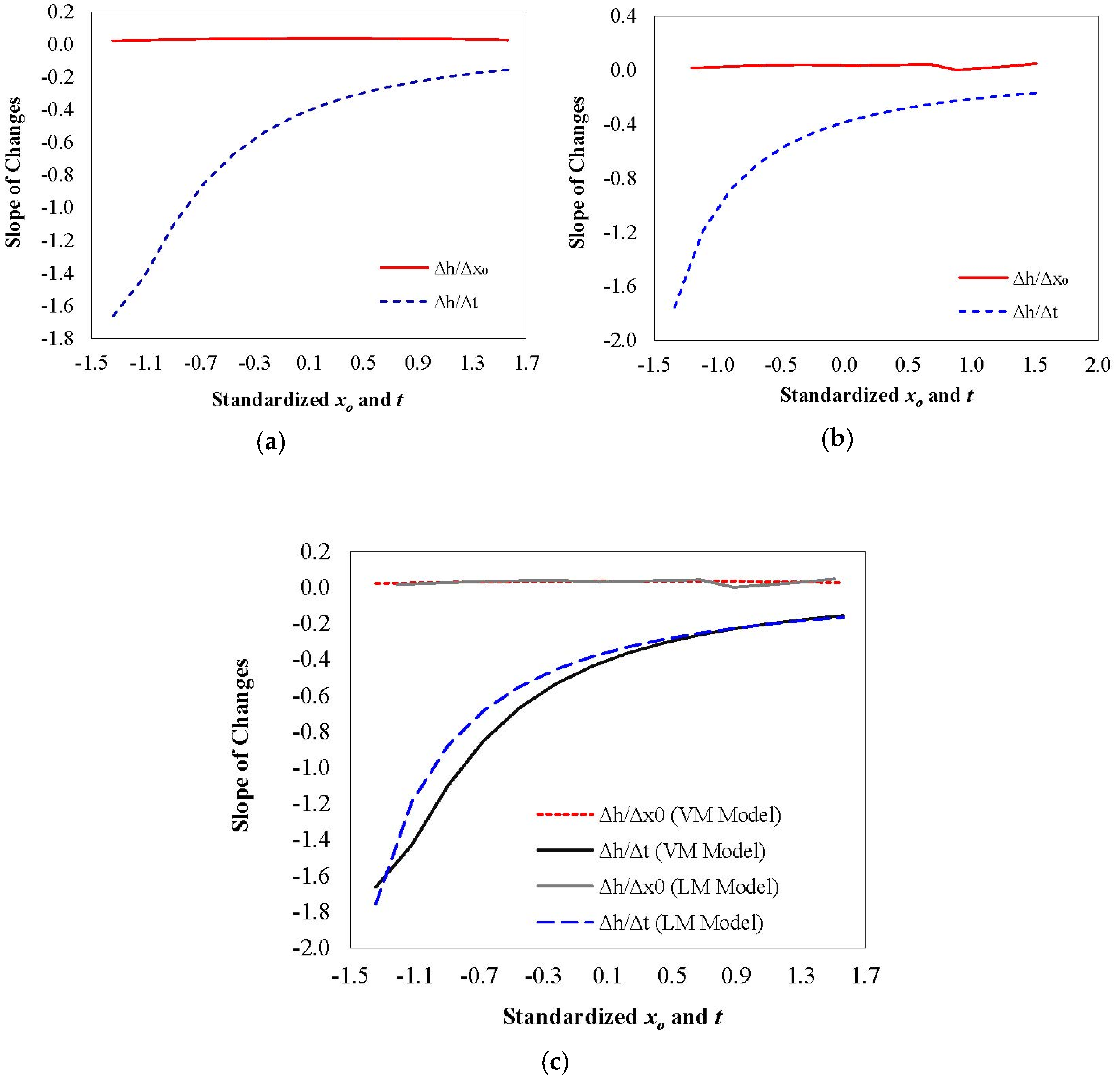
The supernatant–suspension interface height was related to two independent parameters of settling time and initial solid content through an empirical correlation suggested in Equation (11), which is a polynomial functional form:

$$lnh=\alpha +\beta \times \ln \left(t\right)+\gamma \times {\left(\ln \left(t\right)\right)}^2+\delta \times x_0+\epsilon \times {\left(x_0\right)}^2+\theta \times \ln \left(t\right)\times x_0$$

(11)

where $\alpha$, $\beta$, $\gamma$, $\delta$, $\epsilon$, and $\theta$ are the fitting parameters which need to be tuned.

In order to solve this non-linear least square problem, the coefficients were optimized using a standard iterative solution method called Levenberg–Marquardt (LM) algorithm [58,59]. The LM algorithm is basically a numerical method, while the other approach (VM matrix) uses multiple analytical steps to provide reliable results. The present parameter optimization has been used previously in the literature for estimation of hydrate formation temperature as a function of pressure and molecular weight of natural gas [60].

It should be noted that both models may have their own limitations. One of the important drawbacks is related to the application of models in the early stages of sedimentation, where t holds very small values. Indeed, their use at zero time is limited, because when t is equal to zero, the height functions are undefined. Furthermore, more attention should be paid to the reliability of the models at small times. This will be further discussed through error analysis and sensitivity analysis in the results and discussion section.

3.3. Error Analysis

When modeling a physical phenomenon, there is always the chance of introducing some errors into the predictions. Generally, the sources of uncertainty include: perceptual model uncertainty, which reflects the lack of knowledge of different processes involved, data uncertainty (i.e., associated with either the input or output data), parameter uncertainty (i.e., associated with the use of non-optimal parameter values), and model structural uncertainty, which is typically introduced by conceptualizations and simplifications of the descriptions associated with the real-world processes. The discrepancies between direct observations and model predictions originate from the combined impact of all these uncertainty/error sources. Only the uncertainty sources related to the use of non-optimal parameters can be reduced through model calibration [61]. In the current study, there were multiple sources of errors, which are described below:

-

The experimental data of interface height versus time could be subject to measurement error.

-

The interface height versus time curve has various sections with different curvatures. The temporal slopes associated with each particular settling time as well as the changes between the phases can occur at steeper or gentler slopes. In addition, modeling the hindered settling period is a very challenging task.

-

Another source of uncertainty comes from the model’s ability to predict the behavior associated with the experimental data. There is no universal model that could completely capture different behaviors associated with the solid settling phenomenon. If the tuning parameters are not optimally adjusted or insufficient experimental data are utilized, modeling error would increase.

In order to validate the models’ predictions, some statistical parameters were calculated, including coefficient of determination (R²), root mean square error (RMSE), mean absolute percentage error (MAPE), and minimum and maximum of the percentage error (PE). These statistical parameters are defined below [62,63,64,65]:

$$h_{Mean}=\frac{1}{N}{\displaystyle \sum _{i=0}^N{h}_{i,Exp}}$$

(12)

$$R^2=1-\frac{{\displaystyle \sum _{i=1}^N{(h_{i,Exp}-h_{i,\mathrm{Pr}edict})}^2}}{{\displaystyle \sum _{i=1}^N{(h_{i,Exp}-h_{Mean})}^2}}$$

(13)

$$RMSE=\sqrt{\frac{1}{N}{\displaystyle {\sum }_{i=0}^N(}{h}_{i,Exp}-h_{i,\mathrm{Pr}edict}{)}^2}$$

(14)

$$MAPE=\frac{1}{N}{\displaystyle \sum _{i=0}^N\left|\frac{h_{i,Exp}-h_{i,\mathrm{Pr}edict}}{h_{i,Exp}}\right|}\times 100$$

(15)

$$PE=\left|\frac{h_{i,Exp}-h_{i,\mathrm{Pr}edict}}{h_{i,Exp}}\right|\times 100$$

(16)

where N is the number of experimental data, and $h_{i,Exp}$ and $h_{i,\mathrm{Pr}edict}$ introduce the measured and predicted supernatant–suspension interface height, respectively.

As mentioned earlier, the main steps of the modeling procedure in the present study are summarized in Figure 3.

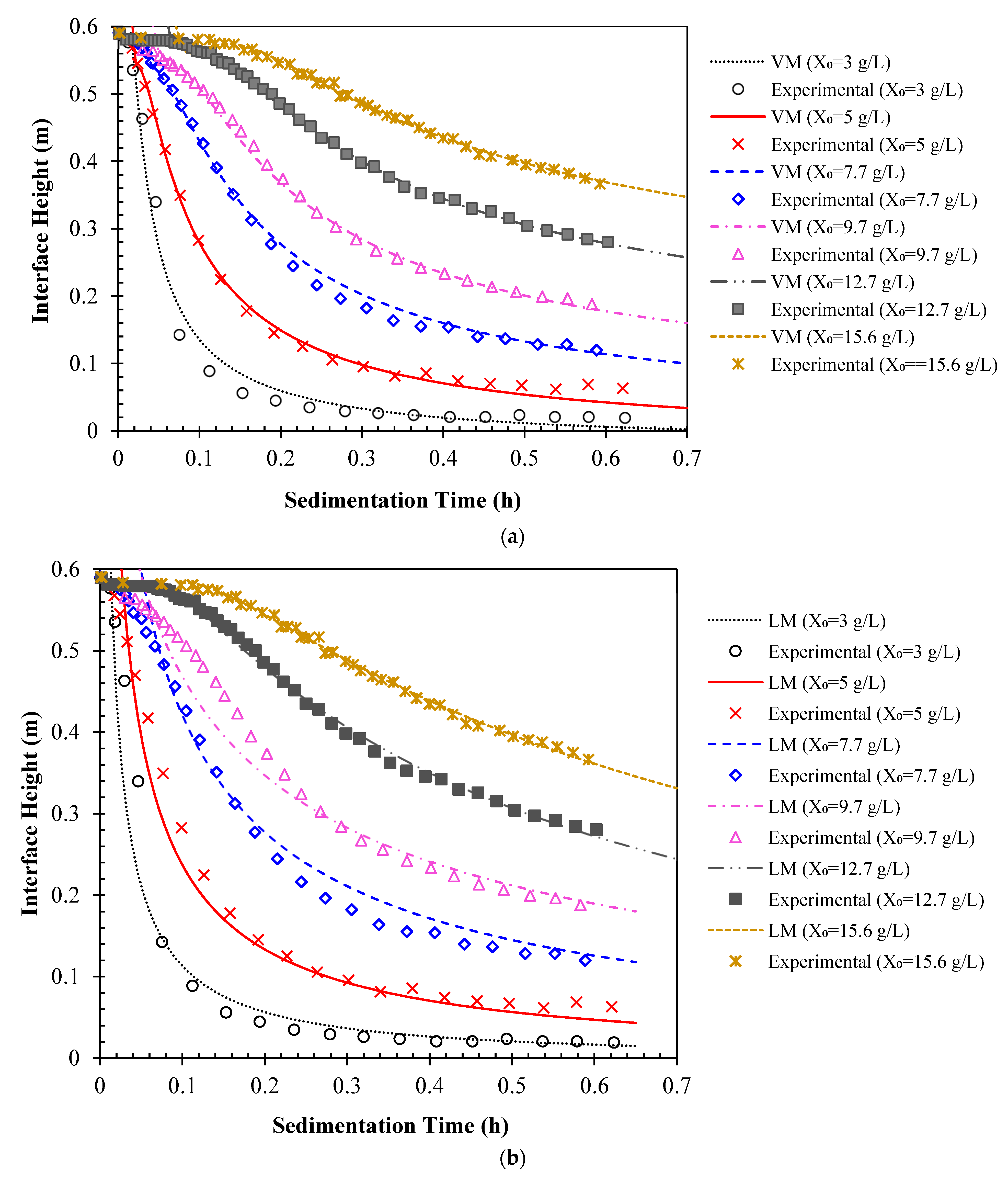
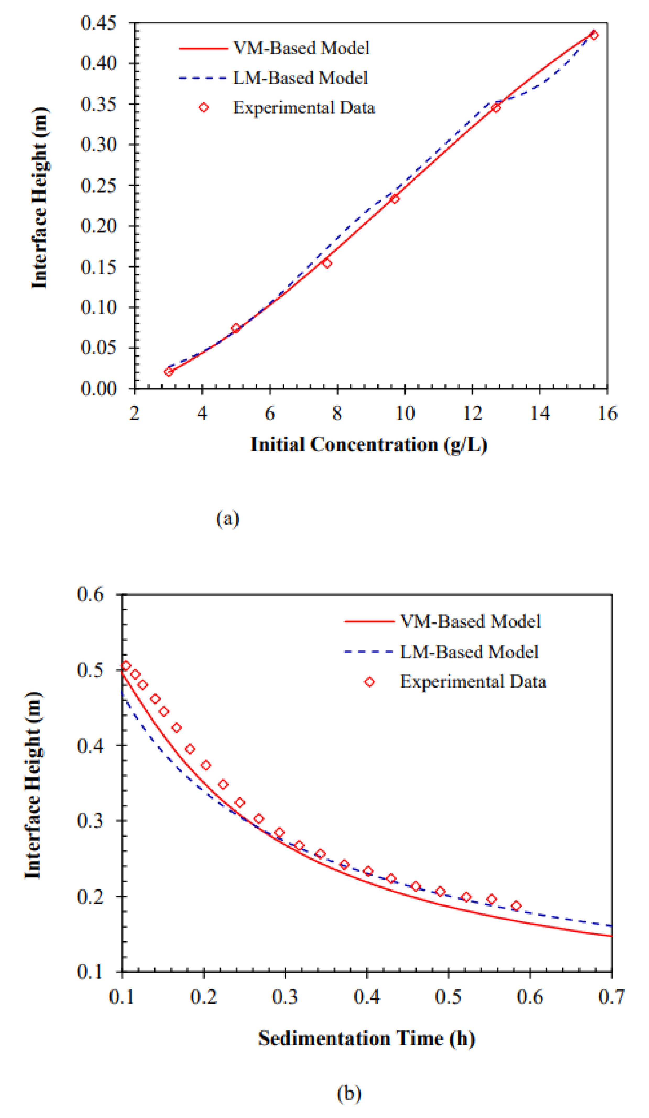
4. Results and Discussion

As discussed in the model development section, the coefficients of both models were tuned in order to fit the experimental data through a parameterization process. The tuned parameters for both correlations are expressed in

Table 1. Tuned coefficients for Equations (7)–(10).

Coefficient	Value
A1	8.077 × 10−3
B1	−0.0176
C1	2.785 × 10−3
D1	−5.99 × 10−5
A2	−0.0103
B2	7.672 × 10−3
C2	5.043 × 10−4
D2	−2.55 × 10−5
A3	−3.659 × 10−4
B3	3.897 × 10−4
C3	−1.025 × 10−4
D3	1.07 × 10−6
A4	3.30 × 10−6
B4	−1.22 × 10−6
C4	−5.41 × 10−7
D4	1.82 × 10−7

and

Table 2. Tuned coefficients for Equation (11).

Coefficient	Value
	x0 < 10.5 g/L	x0 > 10.5 g/L
α	−6.930	0.765
β	0.836	−0.450
γ	−0.0337	0.0202
δ	−1.513	−1.453
ε	−0.0667	−0.152
θ	0.0846	0.0486

, which cover the entire sludge concentration up to 15.6 g/L, and the settling time of up to 0.6 h.

The LM-based model could not predict the sedimentation behavior at all the initial concentrations; therefore, the modeling was performed twice with two concentration ranges. It should be noted that, in dilute suspensions, the solid particles deposit rapidly; therefore, the supernatant–suspension interface height undergoes sharp changes from the initial height to the final sediment thickness. On the contrary, when the initial sludge concentration is greater than a specific value, the sedimentation process occurs much more slowly, and the interface height decreases smoothly due to more significant interactions between the particles. In order to include the shift in sedimentation behavior in our modeling work, it is suggested to calculate the coefficients of the LM-based model twice: once for the concentration range smaller than the critical concentration and another time for solid contents greater than the critical concentration. The critical sludge concentration is defined as the boundary between the high- and low-velocity sedimentation, and can be obtained by trial-and-error procedure with the aim of reducing the error between the predicted and measured data. Wu and Chern [37] as well as Vanderhasselt and Vanrolleghem [21] witnessed this shift in the sedimentation behavior as a function of the sludge concentration. In the present study, the value of 10.5 g/L was used as the critical sludge concentration, which was first introduced by Vanderhasselt and Vanrolleghem. This critical point was the reflex point of the solid flux curve, and was calculated by the Vesilind velocity method [18,37].

For the two empirical correlations introduced in this paper, the experimental data were used to calculate the model parameters. The estimated and measured supernatant–sludge interface height values versus time for various initial sludge concentrations in the range of 3 to 15.6 g/L are plotted in Figure 4. It is clear that both the empirical relations satisfactorily follow the experimental data trends. The greater the initial sludge concentration, the better the match between the estimated and measured data points. On the other hand, the accuracy of the utilized correlations in predicting the measured values deteriorates at smaller initial solid content, especially when the settling velocity increases, and at the transition between the zone settling and compression settling stages. This phenomenon is in agreement with the observations reported in the literature by Vanderhasselt and Vanrolleghem [21]. For any given feed solid concentration, the slope of a tangent to the settling curve from this point represents the settling velocity at that particular solid concentration. Repeating this procedure for different solid concentrations could result in a set of settling velocities to be used for preparation of the solid flux curve as well as unit area calculations for designing thickener units [44]. Each settling curve can be interpreted similarly by looking into three sections of the curve: (1) Constant velocity settling section, which is the initial section of the settling curve, in which the average sedimentation velocity is relatively constant; (2) Hindered or zone settling section, in which the solid settling velocity is progressively reduced, and; (3) Compression settling section, which is the final section of the sedimentation process associated with late settling durations in which the settling velocity is a very small constant. These settling sections are schematically shown in Figure 5. The different zones specified with distinct colors in each settling column from top to bottom are attributed to various “clarity” zones, namely, clarified zone (i.e., supernatant), uniform settling zone, thickening zone, and compressed zone, respectively [66,67].

When the solid concentration in a suspension is increased, there exists a threshold beyond which the particles can no longer settle independently because of their proximity to each other, which also causes the velocity fields of the fluid, displaced by the adjacent particles, to overlap. In such circumstances, there is also a net upward flow of the liquid displaced by the settling particles. All these factors result in reduced particle-settling velocity, also known as “hindered settling”. The most commonly encountered form of hindered settling occurs in an extreme case where the solid particles are so extremely concentrated that the whole suspension tends to settle as a “blanket” This is called “zone settling” because it is possible to distinguish several distinct zones, separated by concentration discontinuities [66,67].

It was also observed that, at greater initial concentrations of the suspensions, the interface height variations during solid settlement are smoother because of the intense interactions between the particles. However, the initial concentration seems to be the most important independent parameter for more-dilute suspensions as well as during the early stages of the settling process; therefore, much bigger deviations between the measured and predicted interface height values are noticed.

The estimation accuracy of the settling performance could also be realized by looking into the parity plots presented in Figure 6. The VM-based model appears to reliably predict the measured solid settling data points; however, for the estimations obtained using the LM-based correlation, some data scatter away from the 1:1 corresponding line, which makes this model less reliable in estimating settling behavior.

The residual errors for settling behavior estimations were also calculated for both the correlations introduced in this study, and are plotted versus the initial sludge concentration as well as time in Figure 7. It is clear that both the correlations resulted in less accurate estimations of settling behavior at smaller initial sludge concentrations (i.e., 3, 5, and 7.7 g/L) compared to greater initial concentrations of 9.7, 12.7, and 15.6 g/L, where the estimations are much closer to the measured data. In addition, the errors in estimations appear to be more pronounced at early settling process times, especially for the LM-based correlation. At higher settling process times and for greater initial sludge concentration, both models appear to perform very well in estimating the measured solid settling behavior. Considering the residual error plots, the VM-based model proved to be more reliable compared to the LM-based model in capturing the solid settling behavior specific to this selected experimental dataset.

Based on the presented error propagations and the physics of the solid settling process, the errors associated with these estimations can be discussed as follows: both correlations performed acceptably through the whole time domain, with the exception of the start of the settling process (i.e., t values close to zero), where both functions become infinite. This problem is rectified when the height estimations are performed at an infinitesimal time value at which the interface height is known. The second source of error could be the very sharp changes in the slope of the supernatant–suspension interface height versus time profile at early settling periods, especially for smaller initial sludge concentrations (i.e., more-dilute suspensions). The performance of both correlations in estimating the settling behavior under such circumstances appears to be less reliable. However, at greater initial solid content of the sludge (i.e., concentrated suspensions), the interface height decreases with a smaller slope due to the significant interactions between the solid particles. To minimize concentration-related error, LM-based model coefficients were determined twice for low and high initial solid concentrations. Even with this modification regarding concentration-dependent parameter tuning, the LM-based correlation still appeared to perform better at greater solid concentrations. This issue was not experienced when working with the VM-based correlation, which resulted in more-accurate estimations without the need for multiple parameters tuning at various initial sludge concentrations.

The accuracy of interface change estimations can be reviewed from another perspective of calculating some statistical parameters for both correlations, as displayed in

Table 3. Statistical parameters for the two correlations.

Model	R2	RMSE	Minimum Percentage Error	Maximum Percentage Error	% MAPE
VM-based model	0.997	0.132	4.869 × 10−4	74.077	5.413
LM-based model	0.969	0.107	0.026	36.59	6.433

. All the statistical indicators for the VM-based model show its superior performance compared to the LM-based correlation.

In order to study the isolated effect of each individual input parameter on the interface height target function, an approach was adopted here where one input parameter was set at its mean value while the second parameter was continuously increased [68,69]. The results of this sensitivity analysis are presented in Figure 8. The greater the slope of each curve, the greater the impact of the varying input parameter on the interface height change. From a qualitative comparison of these two plots, it is apparent that both the predictive methods developed in this paper have the same trend when it comes to the impact of interface height on independent input parameters. In addition, it is evident that “time” has a more pronounced impact on the interface height than “initial concentration” when the other input parameter remains unchanged.

To quantitatively compare the independent effect of each input parameter, the temporal slope of each curve can be calculated using Equation (17):

$$slope\left(h\right)=\frac{\mathsf{\Delta }h}{\mathsf{\Delta }x}$$

(17)

where h and x refer to the interface height and single input parameter (i.e., initial concentration or time), respectively.

The quantitative comparison between the independent input parameters’ impact on the interface height function can be displayed on a single plot when the independent input parameter, shown on the x-axis, is normalized according to the following equation:

$$x_s=\frac{\left(x_i-x_{Mean}\right)}{Std}$$

(18)

where $x_s$, $x_i$, $x_{Mean}$, and std introduce the standardized input parameter, the i^th input parameter, mean of input parameter, and standard deviation of input parameter, respectively.

The comparisons between the independent impacts of each input parameter on the interface height based on various model applications are plotted in Figure 9, where the x-axis in all these plots represents the standard input parameter and the y-axis shows the slope change associated with the interface height extracted from Figure 8. The quantitative comparison presented here also shows that the “time” has a more pronounced impact on the interface height variation than “initial concentration”. The effect of time seems more significant during the early stages of the sedimentation process. The interface height seems less dependent on the initial solid concentration. The LM-based model predictions seem more sensitive to “time” than those of the VM-based model. However, with respect to the initial solid content, both predictive models exhibit similar neutral sensitivity.

5. Conclusions

Sedimentation is a key mechanism commonly used in water and wastewater-treatment plants, at different stages from grit removal to secondary sedimentation and sludge thickening, in order to separate liquid and solids. Prediction of sludge settling behavior is beneficial for design of a thickener or clarifier. In this research work, a modeling study was conducted on the performance of sludge settling process using two simple empirical correlations and experimental data borrowed from the literature. The sedimentation time and initial sludge concentration were the two independent parameters, and the supernatant–sludge interface height was considered as the dependent variable of the process. The predictions generated from both the empirical correlations satisfactorily followed the trends exhibited in the experimental data. The VM-based correlation provided superior performance compared to the LM-based model in terms of better statistical parameters as well as residual error propagation analysis, without a need for multiple tuning of the model parameters as a function of the initial sludge concentration. However, the settling process performance predictions obtained using the LM-based correlation still had acceptable accuracy considering the statistical performance indicators as well as the residual error analysis. It was also observed that the interface height is more sensitive to changes in the settling time than those of the initial sludge concentration. In general, the LM-based model seemed slightly more sensitive to changes in the input parameters than the VM-based model. The benefits of using these simple yet reliable correlations compared to lab- or pilot-scale experimentations are fast computation time, reduction in measurement errors, and high accuracy when the model parameters are properly tuned with some benchmark measured data. The proposed correlations provided a well-behaved (i.e., smooth and non-oscillatory) solution methodology with exemplary statistical indicators when compared to the experimental data. The findings of the present study can be applicable in simulation of the sludge settling behavior in secondary clarifiers and thickeners in biological wastewater-treatment processes, chemical treatment processes of water and wastewater, and also in mineral processing. However, generating the solid flux curve using the proposed relationships for the sludge height as a function of the settling time and initial sludge concentration requires further research. In addition, the present work was performed using the activated sludge data, and further research work is required using other sedimentation data points (i.e., sludge settlement through chemical precipitation, etc.) in order to generalize the proposed approach.

References

1. Rasouli, S.; Rezaei, N.; Hamedi, H.; Zendehboudi, S.; Duan, X. Superhydrophobic and superoleophilic membranes for oil-water separation application: A comprehensive review. Mater. Des. 2021, 204, 109599. [Google Scholar] [CrossRef]
2. Hamedi, H.; Ehteshami, M.; Mirbagheri, S.A.; Rasouli, S.A.; Zendehboudi, S. Current Status and Future Prospects of Membrane Bioreactors (MBRs) and Fouling Phenomena: A Systematic Review. Can. J. Chem. Eng. 2018, 97, 32–58. [Google Scholar] [CrossRef] [Green Version]
3. Metcalf, W.; Eddy, C. Wastewater Engineering, 4th ed.; Mcgraw-Hill Inc.: New York, NY, USA, 2003. [Google Scholar]
4. Kynch, G.J. A theory of sedimentation. Trans. Faraday Soc. 1952, 48, 166–176. [Google Scholar] [CrossRef]
5. Li, B.; Stenstrom, M.K. Dynamic one-dimensional modeling of secondary settling tanks and design impacts of sizing decisions. Water Res. 2014, 50, 160–170. [Google Scholar] [CrossRef]
6. Li, B.; Stenstrom, M.K. Construction of analytical solutions and numerical methods comparison of the ideal continuous settling model. Comput. Chem. Eng. 2015, 80, 211–222. [Google Scholar] [CrossRef]
7. Li, B.; Stenstrom, M. Research advances and challenges in one-dimensional modeling of secondary settling Tanks—A critical review. Water Res. 2014, 65, 40–63. [Google Scholar] [CrossRef] [PubMed]
8. Plósz, B.G.; Weiss, M.; Printemps, C.; Essemiani, K.; Meinhold, J. One-dimensional modelling of the secondary clarifier-factors affecting simulation in the clarification zone and the assessment of the thickening flow dependence. Water Res. 2007, 41, 3359–3371. [Google Scholar] [CrossRef] [PubMed]
9. Bürger, R.; Diehl, S.; Nopens, I. A Consistent Modelling Methodology for Secondary Settling Tanks in Wastewater Treatment. Water Res. 2011, 45, 2247–2260. [Google Scholar] [CrossRef]
10. Bürger, R.; Diehl, S.; Farås, S.; Nopens, I.; Torfs, E. A consistent modelling methodology for secondary settling tanks: A reliable numerical method. Water Sci. Technol. 2013, 68, 192–208. [Google Scholar] [CrossRef] [Green Version]
11. Bürger, R.; Diehl, S.; Mejías, C. On time discretizations for the simulation of the batch settling–compression process in one dimension. Water Sci. Technol. 2015, 73, 1010–1017. [Google Scholar] [CrossRef]
12. Torfs, E.; Maere, T.; Bürger, R.; Diehl, S.; Nopens, I. Impact on Sludge Inventory and Control Strategies Using the Bench-mark Simulation Model No. 1 with the Bürger-Diehl Settler Model. Water Sci. Technol. 2015, 71, 1524–1535. [Google Scholar] [CrossRef] [Green Version]
13. Coe, H.; Clevenger, G. Methods for Determining the Capacities of Slime Settling Tanks. Trans. Am. Inst. Min. Eng. 1916, 55, 356–384. [Google Scholar]
14. Hassett, N.J. Design and Operation of Continuous Thickeners. Ind. Chem. 1958, 34, 116–120. [Google Scholar]
15. Talmage, W.P.; Fitch, E.B. Determining Thickener Unit Areas. Ind. Eng. Chem. 1955, 47, 38–41. [Google Scholar] [CrossRef]
16. Yoshioka, N.; Hotta, Y.; Tanaka, S.; Naito, S.; Tsugami, S. Continuous Thickening of Homogeneous Flocculated Slurries. Chem. Eng. 1957, 21, 66–74. [Google Scholar] [CrossRef] [Green Version]
17. Diehl, S. Estimation of the batch-settling flux function for an ideal suspension from only two experiments. Chem. Eng. Sci. 2007, 62, 4589–4601. [Google Scholar] [CrossRef]
18. Vesilind, P.A. Design of Prototype Thickeners from Batch Settling Tests. Water Sew. Work. 1968, 115, 302–307. [Google Scholar]
19. Zhang, D.; Li, Z.; Lu, P.; Zhang, T.; Xu, D. A method for characterizing the complete settling process of activated sludge. Water Res. 2006, 40, 2637–2644. [Google Scholar] [CrossRef]
20. Cho, S.; Colin, F.; Sardin, M.; Prost, C. Settling velocity model of activated sludge. Water Res. 1993, 27, 1237–1242. [Google Scholar] [CrossRef]
21. Vanderhasselt, A.; Vanrolleghem, P.A. Estimation of Sludge Sedimentation Parameters from Single Batch Settling Curves. Water Res. 2000, 34, 395–406. [Google Scholar] [CrossRef]
22. Turlej, T. Automation of sedimentation test. Water Sci. Technol. 2018, 77, 1960–1966. [Google Scholar] [CrossRef] [PubMed]
23. Singh, K.M.P.; Udayabhanu, G.; Gouricharan, T. Comparative Studies on The Settling Behavior of Indian Noncoking Coal Fines by Standard Jar Test and Instrument Au. Int. L. J. Coal. Prep. Util. 2014, 34, 65–74. [Google Scholar] [CrossRef]
24. Guerin, M.; Seaman, J.C. Characterizing Clay Mineral Suspensions Using Acoustic and Electroacoustic Spectroscopy—A Review. Clays Clay Miner. 2004, 52, 145–157. [Google Scholar] [CrossRef]
25. Vergouw, J.; Anson, J.; Dalhke, R.; Xu, Z.; Gomez, C.; Finch, J. An automated data acquisition technique for settling tests. Miner. Eng. 1997, 10, 1095–1105. [Google Scholar] [CrossRef]
26. Hunter, T.; Peakall, J.; Biggs, S. Ultrasonic velocimetry for the in situ characterisation of particulate settling and sedimentation. Miner. Eng. 2011, 24, 416–423. [Google Scholar] [CrossRef]
27. Kaushal, D.; Tomita, Y. Experimental investigation for near-wall lift of coarser particles in slurry pipeline using γ-ray densitometer. Powder Technol. 2007, 172, 177–187. [Google Scholar] [CrossRef]
28. Hoffman, D.L.; Brooks, D.R.; Dolez, P.I.; Love, B.J. Design of A Z-Axis Translating Laser Light Scattering Device For Par-ticulate Settling Measurement In Dispersed Fluids. Rev. Sci. Instrum. 2002, 73, 2479–2482. [Google Scholar] [CrossRef] [Green Version]
29. Hernando, L.; Omari, A.; Reungoat, D. Experimental study of sedimentation of concentrated mono-disperse suspensions: Determination of sedimentation modes. Powder Technol. 2014, 258, 265–271. [Google Scholar] [CrossRef]
30. Lu, X.; Liao, Z.; Li, X.; Wang, M.; Wu, L.; Li, H.; York, P.; Xu, X.; Yin, X.; Zhang, J. Automatic monitoring and quantitative characterization of sedimentation dynamics for non-homogenous systems based on image profile analysis. Powder Technol. 2015, 281, 49–56. [Google Scholar] [CrossRef]
31. Kołodziejczyk, K. Numerical simulation of polydispersed suspension sedimentation under flow conditions Symulacja numeryczna procesu sedymentacji zawiesiny polidyspersyjnej w układzie przepływowym. Przem. Chem. 2016, 1, 66–69. [Google Scholar] [CrossRef]
32. Nocoń, W. Quantitative monitoring of batch sedimentation based on fractional density changes. Powder Technol. 2016, 292, 1–6. [Google Scholar] [CrossRef]
33. Acosta-Cabronero, J.; Hall, L.D. Measurements by Mri of The Settling and Packing of Solid Particles from Aqueous Suspensions. Aiche J. 2009, 55, 1426–1433. [Google Scholar] [CrossRef]
34. Zhu, Y.; Wu, J.; Shepherd, I.; Coghill, M.; Vagias, N.; Elkin, K. An automated measurement technique for slurry settling tests. Miner. Eng. 2000, 13, 765–772. [Google Scholar] [CrossRef]
35. Hubner, T.; Will, S.; Leipertz, A. Sedimentation Image Analysis (SIA) for the Simultaneous Determination of Particle Mass Density and Particle Size. Part. Part. Syst. Charact. 2001, 18, 70–78. [Google Scholar] [CrossRef]
36. Zheng, Y.; Bagley, D.M. Numerical Simulation of Batch Settling Process. J. Environ. Eng. 1999, 125, 1007–1013. [Google Scholar] [CrossRef]
37. Wu, C.-H.; Chern, J.-M. Experiment and Simulation of Sludge Batch Settling Curves: A Wave Approach. Ind. Eng. Chem. Res. 2006, 45, 2026–2031. [Google Scholar] [CrossRef]
38. Grassia, P.; Usher, S.; Scales, P. A simplified parameter extraction technique using batch settling data to estimate suspension material properties in dewatering applications. Chem. Eng. Sci. 2008, 63, 1971–1986. [Google Scholar] [CrossRef]
39. Lester, D.R.; Usher, S.P.; Scales, P.J. Estimation of The Hindered Settling Function R (Φ) From Batch-Settling Tests. Aiche J. 2005, 51, 1158–1168. [Google Scholar] [CrossRef]
40. Grassia, P.; Usher, S.; Scales, P. Closed-form solutions for batch settling height from model settling flux functions. Chem. Eng. Sci. 2011, 66, 964–972. [Google Scholar] [CrossRef]
41. Van Deventer, B.B.; Usher, S.P.; Kumar, A.; Rudman, M.; Scales, P.J. Aggregate densification and batch settling. Chem. Eng. J. 2011, 171, 141–151. [Google Scholar] [CrossRef]
42. Betancourt, F.; Bürger, R.; Diehl, S.; Mejías, C. Advanced methods of flux identification for clarifier–thickener simulation models. Miner. Eng. 2014, 63, 2–15. [Google Scholar] [CrossRef]
43. Van Deventer, B.B.G. Aggregate Densification Behaviour in Sheared Suspensions. Ph.D. Thesis, University of Melbourne, Melbourne, Austrailia, 2012. [Google Scholar]
44. Banisi, S.; Yahyaei, M. Feed Dilution-Based Design of a Thickener for Refuse Slurry of a Coal Preparation Plant. Int. J. Coal Prep. Util. 2008, 28, 201–223. [Google Scholar] [CrossRef]
45. Zhang, L.; Wu, A.; Wang, H.; Wang, L. Representation of batch settling via fitting a logistic function. Miner. Eng. 2018, 128, 160–167. [Google Scholar] [CrossRef]
46. Kang, X.; Xia, Z.; Wang, J.; Yang, W. A Novel Approach to Model the Batch Sedimentation and Estimate the Settling Velocity, Solid Volume Fraction, and Floc Size of Kaolinite in Concentrated Solutions. Colloids Surf. A Physicochem. Eng. Asp. 2019, 579, 123647. [Google Scholar] [CrossRef]
47. Von Sperling, M. Basic Principles of Wastewater Treatment; IWA Publishing: London, UK, 2017. [Google Scholar]
48. Barrott, L.; Ersoz, M. Best Practice Guide on Metals Removal from Drinking Water by Treatment; IWA Publishing: London, UK, 2012. [Google Scholar]
49. Spellman, F.R. Mathematics Manual for Water and Wastewater Treatment Plant Operators: Wastewater Treatment Operations: Math Concepts and Calculations; CRC Press: Boca Raton, FL, USA, 2014. [Google Scholar]
50. Lundengård, K. Generalized Vandermonde Matrices and Determinants. In Electromagnetic Compatibility; Mälardalen University: Västerås, Sweden, 2017. [Google Scholar]
51. Bahadori, A.; Zahedi, G.; Zendehboudi, S.; Bahadori, M. Estimation of Air Concentration in Dissolved Air Flotation (Daf) Sys-Tems Using A Simple Predictive Tool. Chem. Eng. Res. Des. 2013, 91, 184–190. [Google Scholar] [CrossRef]
52. Ghiasi, M.M.; Bahadori, A.; Zendehboudi, S. Estimation of The Water Content of Natural Gas Dried By Solid Calcium Chloride Dehydrator Units. Fuel 2014, 117, 33–42. [Google Scholar] [CrossRef]
53. Ghiasi, M.M.; Bahadori, A.; Zendehboudi, S.; Jamili, A.; Rezaei-Gomari, S. Novel Methods Predict Equilibrium Vapor Metha-Nol Content During Gas Hydrate Inhibition. J. Nat. Gas Sci. Eng. 2013, 15, 69–75. [Google Scholar] [CrossRef]
54. Fulton, W.; Harris, J. Representation Theory: A First Course, Graduate Texts in Mathematics, Readings in Mathematics; Springer: New York, NY, USA, 1991; Volume 129. [Google Scholar]
55. Horn, R.A.; Johnson, C.R. Topics in Matrix Analysis; Cambridge University Press: London, UK, 1991; Volume Section 6.1. [Google Scholar]
56. Bahadori, A.; Zahedi, G.; Zendehboudi, S.; Jamili, A. Estimation of the effect of biomass moisture content on the direct combustion of sugarcane bagasse in boilers. Int. J. Sustain. Energy 2011, 33, 349–356. [Google Scholar] [CrossRef]
57. Amin, J.S.; Alimohammadi, S.; Zendehboudi, S. Systematic investigation of asphaltene precipitation by experimental and reliable deterministic tools. Can. J. Chem. Eng. 2017, 95, 1388–1398. [Google Scholar] [CrossRef]
58. Levenberg, K. A method for the solution of certain non-linear problems in least squares. Q. Appl. Math. 1944, 2, 164–168. [Google Scholar] [CrossRef] [Green Version]
59. Marquardt, D.W. An Algorithm for Least-Squares Estimation of Nonlinear Parameters. J. Soc. Ind. Appl. Math. 1963, 11, 431–441. [Google Scholar] [CrossRef]
60. Ghiasi, M.M. Initial Estimation of Hydrate Formation Temperature of Sweet Natural Gases Based on New Empirical Correlation. J. Nat. Gas Chem. 2012, 21, 508–512. [Google Scholar] [CrossRef]
61. Vanrolleghem, P.A. Modelling Aspects of Water Framework Directive Implementation; IWA Publishing: London, UK, 2010; Volume 1, 260p. [Google Scholar]
62. Chiulli, R.M. Quantitative Analysis: An Introduction; CRC Press: Boca Raton, FL, USA, 1999; Volume 2. [Google Scholar]
63. Millard, S.P.; Neerchal, N.K. Environmental Statistics with S-PLUS; CRC Press: Boca Raton, FL, USA, 2000. [Google Scholar]
64. Bozdogan, H. Statistical Data Mining and Knowledge Discovery; CRC Press: Boca Raton, FL, USA, 2003. [Google Scholar]
65. Everitt, B.; Skrondal, A. The Cambridge Dictionary of Statistics; Cambridge University Press: Cambridge, UK, 2002; ISBN 0-521-81099-X. [Google Scholar]
66. Haan, C.T.; Barfield, B.J.; Hayes, J.C. 7—Sediment Properties and Transport. In Design Hydrology and Sedimentology for Small Catchments; Haan, C.T., Barfield, B.J., Hayes, J.C., Eds.; Academic Press: San Diego, CA, USA, 1994; pp. 204–237. [Google Scholar]
67. Yetilmezsoy, K. A New Empirical Model for The Determination of The Required Retention Time in Hindered Settling. Frese-Nius Environ. Bull. 2007, 16, 674–684. [Google Scholar]
68. Downing, D.J.; Gardner, R.H.; Hoffman, F.O. An Examination of Response-Surface Methodologies for Uncertainty Analysis in Assessment Models. Technometrics 1985, 27, 151–163. [Google Scholar] [CrossRef]
69. Hamby, D.M. A review of techniques for parameter sensitivity analysis of environmental models. Environ. Monit. Assess. 1994, 32, 135–154. [Google Scholar] [CrossRef]
Figure 1. Layout of a conventional wastewater-treatment plant.
Energies 16 00963 g001
Figure 2. Algorithm used for tuning the coefficients associated with the VM-based model (Equations (6)–(10)).
Energies 16 00963 g002
Figure 3. Main steps of the modeling process.
Energies 16 00963 g003
Figure 4. Comparison between the measured solid settling data (borrowed from [21]) and the data predicted using (a) the VM-based model using Equations (6)–(10) and (b) LM-based model using Equation (11).
Energies 16 00963 g004
Figure 5. Different solids settling sections and clarity zones in a typical batch settling column test with initial sludge concentration of 5 g/L.
Energies 16 00963 g005
Figure 6. Parity plots comparing the measured solid settling data, borrowed from [21], with the predicted data using (a) the VM-based model (Equations (6)–(10)) and (b) LM-based model (Equation (11)).
Energies 16 00963 g006
Figure 7. Residual errors between the measured settling behavior, borrowed from [21], and estimated behavior using VM- and LM-based correlations versus initial sludge concentration (a,c) and time (b,d), respectively.
Energies 16 00963 g007
Figure 8. Sensitivity analysis of the isolated effect of (a) initial concentration and (b) time on the interface height while the other input parameter remains constant at its mean value.
Energies 16 00963 g008
Figure 9. Slope changes in “interface height versus input parameter” as a function of the standardized input parameter predicted using (a) VL-based model and (b) LM-based model, and comparison of the two predictions in (c).
Energies 16 00963 g009