

A Robust Optimization Model of Aggregated Resources Considering Serving Ratio for Providing Reserve Power in the Joint Electricity Market

Abstract
:1. Introduction
- We propose a bidding strategy for renewable energy resources and energy storage owned by an aggregator who can participate in both the energy and reserve markets;
- The aggregator can provide reserve power as a percentage of the generation determined in the day-ahead market, and the reserve power can be utilized to increase or decrease generation in the real-time operation;
- Unlike previous studies that only used real-time reserve prices for reserve settlement, this study uses the real-time market price for reserve settlement to pay for increased or decreased generation;
- We introduce an optimization problem based on robust optimization, which considers that uncertainties of renewable energy and power-generation increase and decrease in the real-time operation.
2. Aggregated Resources’ Participation in the Joint Market
2.1. Assumptions
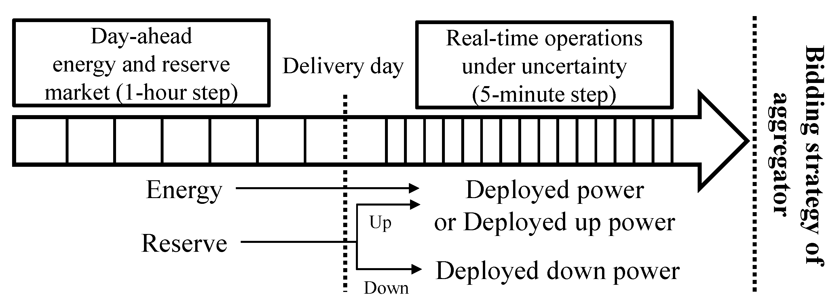
- The day-ahead market structure comprises an energy market and a reserve market as proposed in [25]. The reserve market is a market for trading reserve power to be used on the delivery day. Reserve power is divided into up- and down-reserve power: in the real-time operation, up-reserve power is used to generate additional energy from the planned energy, and down-reserve power is used to decrease the planned energy.
- The aggregator determines the available capacity based on the forecast output in the day-ahead operation and how much of the available capacity can be used to provide reserve power by assessing the serving ratio. The serving ratio applies only to the day-ahead operation and, once determined, does not change in the real-time operation.
- As with [25], by considering the real-time operation, the aggregator can expect to increase or decrease their output within the determined reserve power in the day-ahead market. The system operator can accept any increase or decrease in output from the aggregator.
- The real-time market uses a time step smaller than one hour, as opposed to the day-ahead market, which uses an hourly time step.
- All increases and decreases in output are settled at the real-time market price. However, a decrease in output except for a power imbalance in renewable energy resources between the day-ahead market and real-time operation is settled at the reserve price in the real-time market.
2.2. Participation Model Description
- The aggregator schedules their output to maximize profits by considering the day-ahead market and real-time operation. The aggregator predicts the amount of renewable energy utilized in the real-time operation and the amount of energy and reserves utilized in the electricity market by charging and discharging energy-storage systems;
- The reserve power planned by the day-ahead market is determined by the sum of the hourly forecast power of renewable energy resources and maximum power of energy storage multiplied by the serving ratio for reserve power;
- Uncertainties that cause the difference between the day-ahead market and real-time operation comprise the deployed up/down power and renewable energy in the real-time operation.
3. Robust Optimization Model for Aggregated Resources Considering the Serving Ratio
3.1. Objective Function
- Constraints on day-ahead energy schedule:
- Constraints on day-ahead reserve schedule:
- Constraints on deployed up and down power in the real-time operation:
- Constraints on power imbalance of renewable energy resources:
3.2. Operation Constraints
- Constraints on energy storage operation:
- Operation constraints on charging of energy storage:
- Operation constraints on discharging of energy storage:
- Operation constraints on stored energy of energy storage:
- Operation constraints on renewable energy resources:
3.3. Serving Ratio for Reserve Power
3.4. Robust Optimization Model
- Constraints on uncertain parameters:
- Formulation of the robust optimization problem:
4. Case Study
4.1. Main Assumptions
4.2. Simulation Results
4.2.1. Case Description
4.2.2. Case 1: Results without Considering Uncertain Parameters (0% Variation Interval)
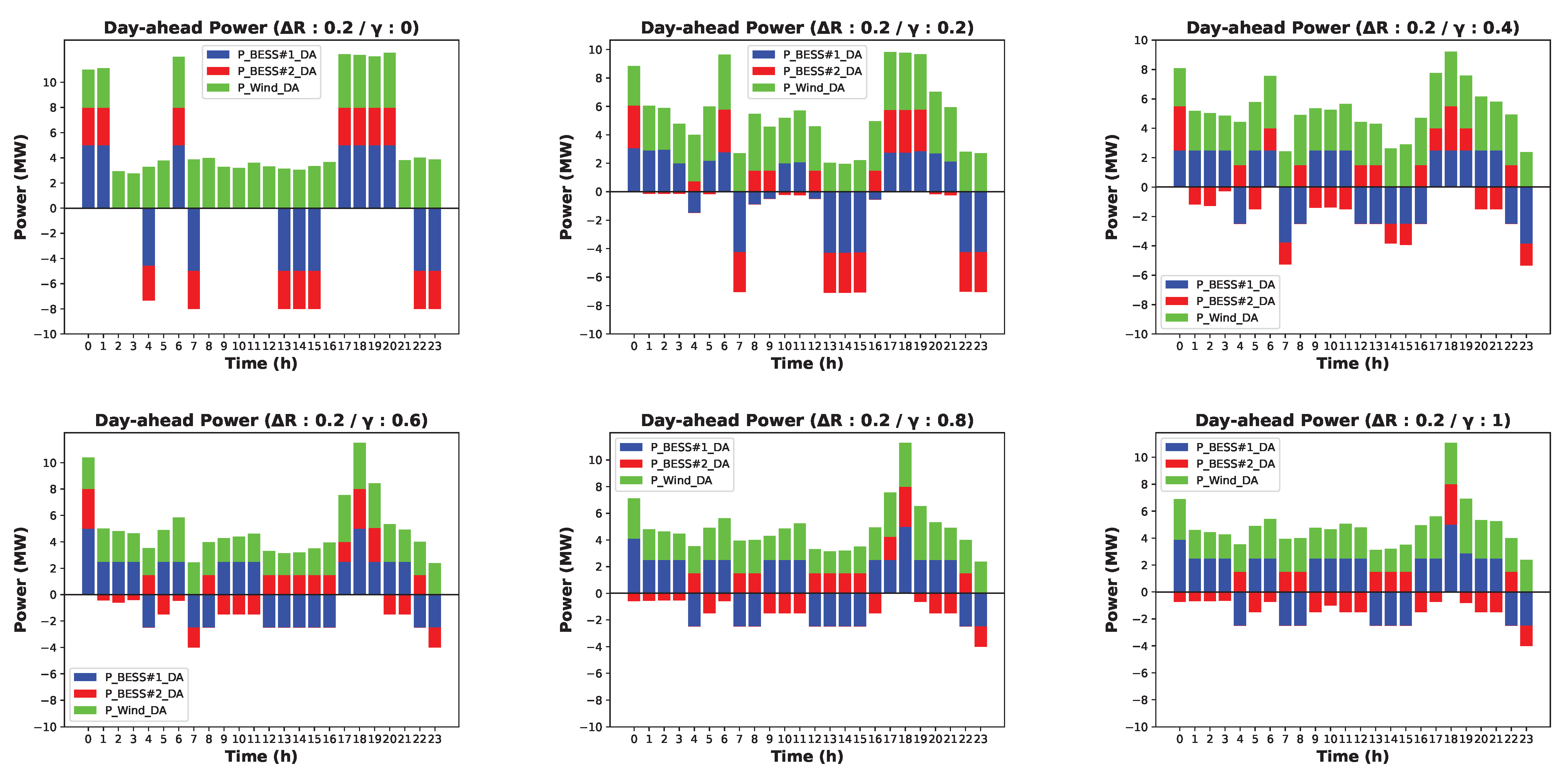
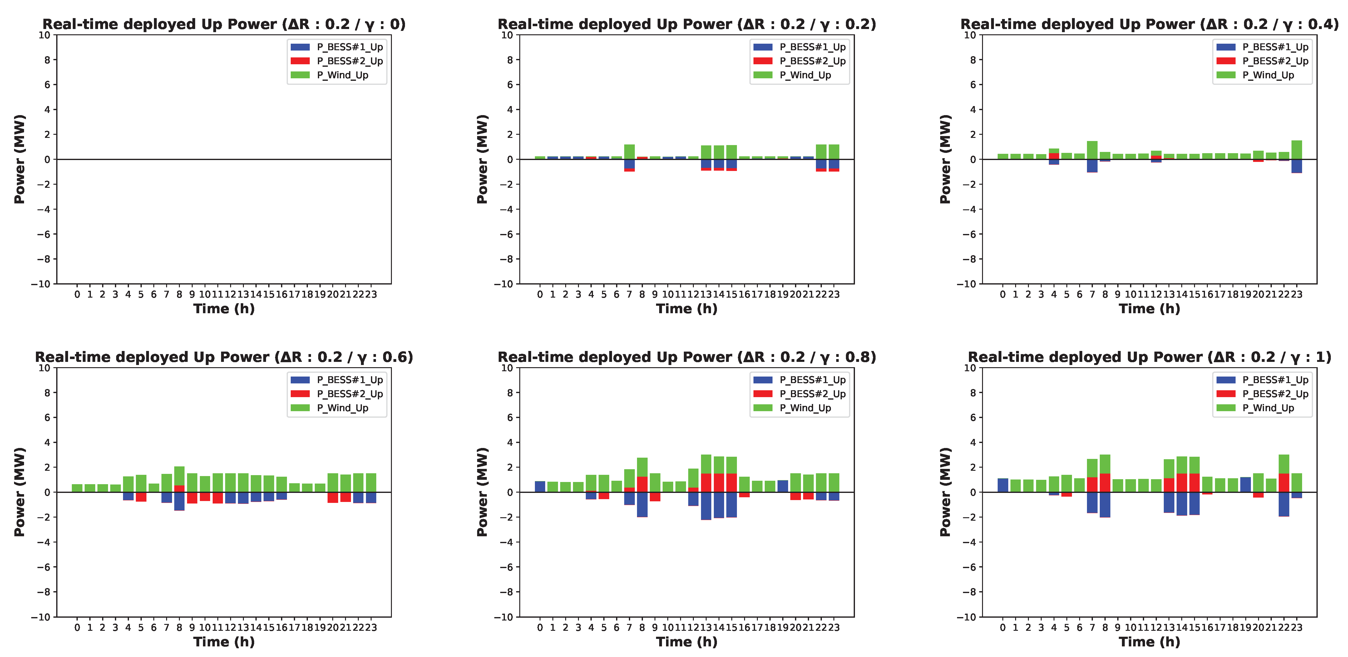
4.2.3. Case 2: Results with Considering Uncertain Parameters (−20∼20% Variation Interval)
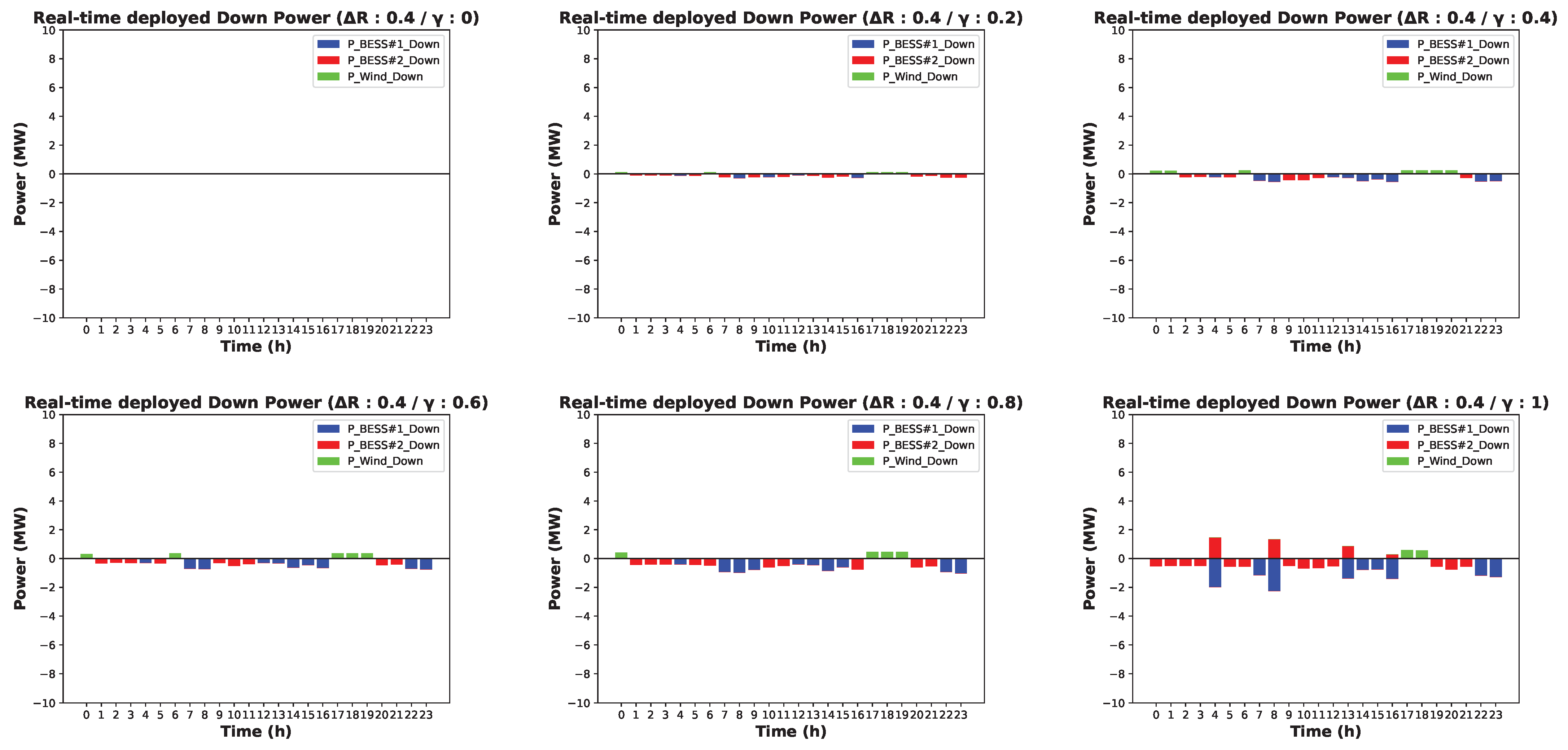
4.2.4. Case 3: Results with Considering Uncertain Parameters (−40∼40% Variation Interval)
5. Discussion
6. Conclusions
Author Contributions
Funding
Data Availability Statement
Conflicts of Interest
Nomenclature
| Abbreviation: | |
| Day-ahead | |
| Real-time | |
| Charging operation of energy storage | |
| Discharging operation of energy storage | |
| Renewable energy resource | |
| Indices and Sets: | |
| t, , T | Index, number of set, and set of hourly time category |
| j(), , J | Index, number of set, and set of intra-hourly time category |
| s, , S | Index, number of set, and set of energy storage |
| r, , R | Index, number of set, and set of renewable energy resources |
| Parameters: | |
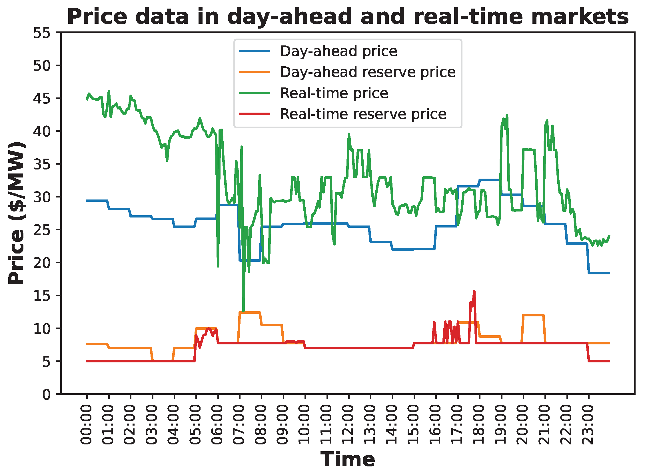
| Day-ahead prices | |
| Day-ahead reserve prices | |
| Real-time prices | |
| Real-time reserve prices | |
| , | Marginal cost of energy storage sth in charging and discharging modes |
| Marginal cost of renewable energy resources rth | |
| Ramp-rate of energy storage sth | |
| Ramp-rate of renewable energy resources rth | |
| , | Minimum and maximum power of energy storage sth |
| , | Minimum and maximum energy of energy storage sth |
| Variation interval for uncertain parameters | |
| Expected power generation of renewable energy resources rth in the real-time operation | |
| Serving ratio for reserve power | |
| Duration of intra-hourly interval | |
| Variables: | |
| , | Selling and buying bids in the day-ahead energy market |
| Reserve bids in the day-ahead reserve market | |
| , | Deployed up and down power from the reserve power in the real-time operation |
| , | Day-ahead scheduling of energy storage sth in charging and discharging modes in the day-ahead energy market |
| Day-ahead scheduling of renewable energy resources rth in the day-ahead energy market | |
| , | Reserve scheduling of energy storage sth in charging and discharging modes in the day-ahead reserve market |
| Reserve scheduling of renewable energy resources rth in the day-ahead reserve market | |
| , | Deployed charging power from the reserve power of energy storage sth in the real-time up and down operation |
| , | Deployed discharging power from the reserve power of energy storage sth in the real-time up and down operation |
| , | Deployed power from the reserve power of renewable energy resources rth in the real-time up and down operation |
| Stored energy of energy storage sth | |
| Power imbalance of renewable energy resources rth between the day-ahead market and real-time operation | |
| Actual power generation of renewable energy resources rth in the real-time operation | |
| Auxiliary variable of robust optimization | |
| Binary Variables: | |
| , | Charging and discharging binary variables of energy storage sth |
| Commitment status binary variable of renewable energy resources rth |
References
- Nyangon, J.; Byrne, J. Estimating the impacts of natural gas power generation growth on solar electricity development: PJM’s evolving resource mix and ramping capability. Wires Energy Environ. 2023, 12, e454. [Google Scholar] [CrossRef]
- Nyangon, J.; Byrne, J. Spatial Energy Efficiency Patterns in New York and Implications for Energy Demand and the Rebound Effect. Energy Sources Part B Econ. Plan. Policy 2021, 16, 135–161. [Google Scholar] [CrossRef]
- Byrne, J.; Taminiau, J.; Nyangon, J. American policy conflict in the hothouse: Exploring the politics of climate inaction and polycentric rebellion. Energy Res. Soc. Sci. 2022, 89, 102551. [Google Scholar] [CrossRef]
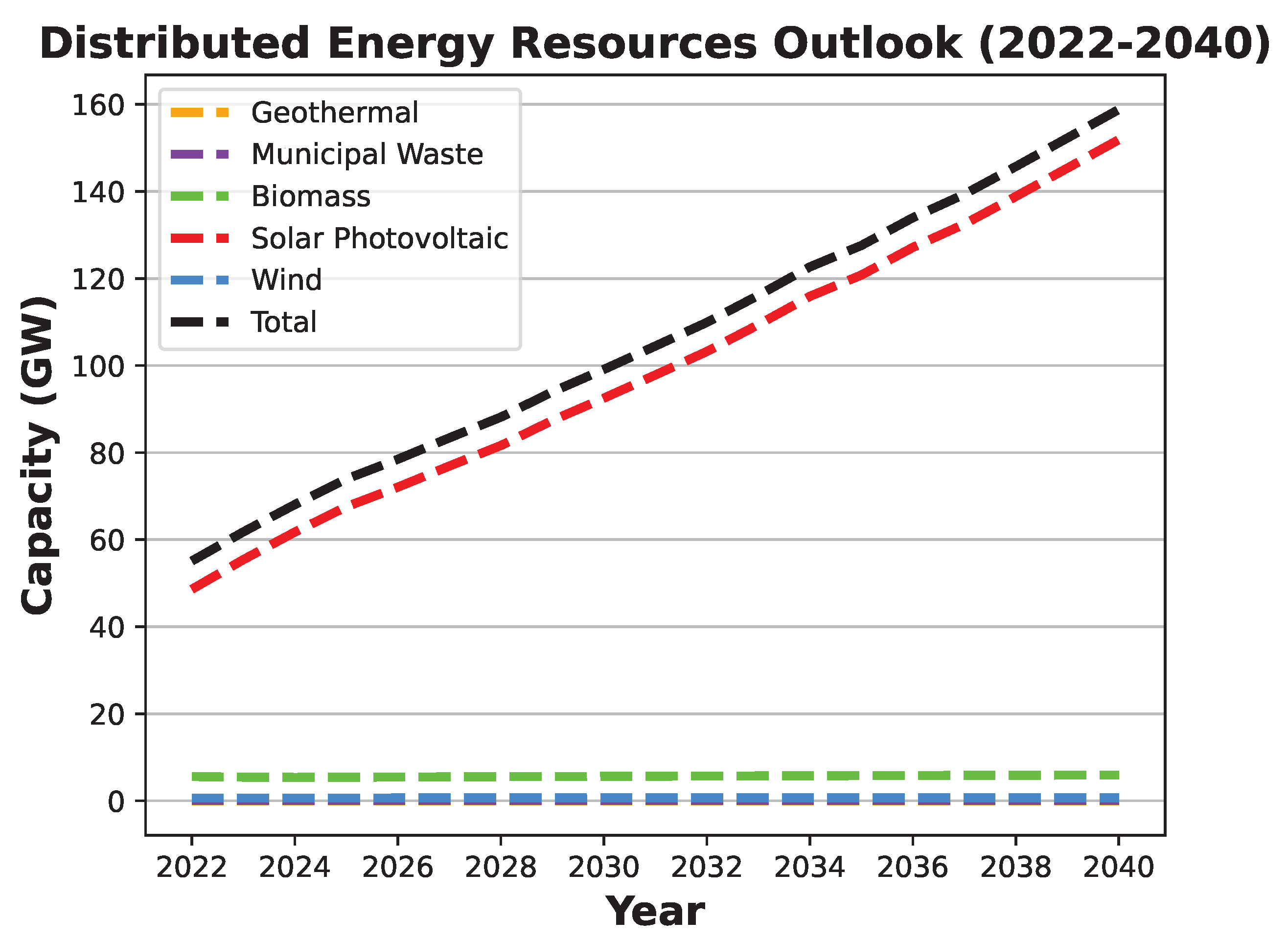
- Annual Energy Outlook 2023—Renewable Energy Generating Capacity and Generation. Available online: https://www.eia.gov/outlooks/aeo/data/browser/#/?id=16-AEO2023®ion=0-0&cases=ref2023&start=2021&end=2040&f=A&linechart=~~~~~~~~~~~~~~~~~~~~~~~~~~~~~~~~~~~ref2023-d020623a.30-16-AEO2023~ref2023-d020623a.31-16-AEO2023~ref2023-d020623a.32-16-AEO2023~ref2023-d020623a.33-16-AEO2023~ref2023-d020623a.34-16-AEO2023~ref2023-d020623a.35-16-AEO2023~&ctype=linechart&chartindexed=0&sourcekey=0 (accessed on 19 September 2023).
- Wu, C.; Zhang, X.P.; Sterling, M. Solar power generation intermittency and aggregation. Sci. Rep. 2022, 12, 1363. [Google Scholar] [CrossRef]
- Castagneto Gissey, G.; Subkhankulova, D.; Dodds, P.E.; Barrett, M. Value of energy storage aggregation to the electricity system. Energy Policy 2019, 128, 685–696. [Google Scholar] [CrossRef]
- Ntomaris, A.V.; Marneris, I.G.; Biskas, P.N.; Bakirtzis, A.G. Optimal participation of RES aggregators in electricity markets under main imbalance pricing schemes: Price taker and price maker approach. Electr. Power Syst. Res. 2022, 206, 107786. [Google Scholar] [CrossRef]
- Han, X.; Hug, G. A distributionally robust bidding strategy for a wind-storage aggregator. Electr. Power Syst. Res. 2020, 189, 106745. [Google Scholar] [CrossRef]
- Khojasteh, M.; Faria, P.; Lezama, F.; Vale, Z. A novel adaptive robust model for scheduling distributed energy resources in local electricity and flexibility markets. Appl. Energy 2023, 342, 121144. [Google Scholar] [CrossRef]
- Silva-Rodriguez, L.; Sanjab, A.; Fumagalli, E.; Virag, A.; Gibescu, M. A light robust optimization approach for uncertainty-based day-ahead electricity markets. Electr. Power Syst. Res. 2022, 212, 108281. [Google Scholar] [CrossRef]
- Wang, F.; Ge, X.; Yang, P.; Li, K.; Mi, Z.; Siano, P.; Duić, N. Day-ahead optimal bidding and scheduling strategies for DER aggregator considering responsive uncertainty under real-time pricing. Energy 2020, 213, 118765. [Google Scholar] [CrossRef]
- Edmunds, C.; Martín-Martínez, S.; Browell, J.; Gómez-Lázaro, E.; Galloway, S. On the participation of wind energy in response and reserve markets in Great Britain and Spain. Renew. Sustain. Energy Rev. 2019, 115, 109360. [Google Scholar] [CrossRef]
- Zhang, R.; Sun, H.; Li, G.; Jiang, T.; Li, X.; Chen, H.; Zou, H. Reserve provision of combined-cycle unit in joint day-ahead energy and reserve markets. Appl. Energy 2023, 336, 120812. [Google Scholar] [CrossRef]
- Tavakkoli, M.; Fattaheian-Dehkordi, S.; Pourakbari-Kasmaei, M.; Liski, M.; Lehtonen, M. An Approach to Divide Wind Power Capacity Between Day-Ahead Energy and Intraday Reserve Power Markets. IEEE Syst. J. 2022, 16, 1123–1134. [Google Scholar] [CrossRef]
- Sun, G.; Shen, S.; Chen, S.; Zhou, Y.; Wei, Z. Bidding strategy for a prosumer aggregator with stochastic renewable energy production in energy and reserve markets. Renew. Energy 2022, 191, 278–290. [Google Scholar] [CrossRef]
- Yang, C.; Du, X.; Xu, D.; Tang, J.; Lin, X.; Xie, K.; Li, W. Optimal bidding strategy of renewable-based virtual power plant in the day-ahead market. Int. J. Electr. Power Energy Syst. 2023, 144, 108557. [Google Scholar] [CrossRef]
- Chen, H.; Wang, D.; Zhang, R.; Jiang, T.; Li, X. Optimal participation of ADN in energy and reserve markets considering TSO-DSO interface and DERs uncertainties. Appl. Energy 2022, 308, 118319. [Google Scholar] [CrossRef]
- Duan, X.; Hu, Z.; Song, Y. Bidding Strategies in Energy and Reserve Markets for an Aggregator of Multiple EV Fast Charging Stations With Battery Storage. IEEE Trans. Intell. Transp. Syst. 2021, 22, 471–482. [Google Scholar] [CrossRef]
- Mi, Z.; Jia, Y.; Wang, J.; Zheng, X. Optimal Scheduling Strategies of Distributed Energy Storage Aggregator in Energy and Reserve Markets Considering Wind Power Uncertainties. Energies 2018, 11, 1242. [Google Scholar] [CrossRef]
- Iria, J.; Soares, F. Real-time provision of multiple electricity market products by an aggregator of prosumers. Appl. Energy 2019, 255, 113792. [Google Scholar] [CrossRef]
- Xia, Y.; Xu, Q.; Huang, Y.; Du, P. Peer-to-peer energy trading market considering renewable energy uncertainty and participants’ individual preferences. Int. J. Electr. Power Energy Syst. 2023, 148, 108931. [Google Scholar] [CrossRef]
- Manna, C.; Sanjab, A. A decentralized stochastic bidding strategy for aggregators of prosumers in electricity reserve markets. J. Clean. Prod. 2023, 389, 135962. [Google Scholar] [CrossRef]
- Bahramara, S.; Sheikhahmadi, P.; Chicco, G.; Mazza, A.; Wang, F.; Catalão, J.P.S. Modeling the Microgrid Operator Participation in Day-Ahead Energy and Reserve Markets Considering Stochastic Decisions in the Real-Time Market. IEEE Trans. Ind. Appl. 2022, 58, 5747–5762. [Google Scholar] [CrossRef]
- Kuttner, L. Integrated scheduling and bidding of power and reserve of energy resource aggregators with storage plants. Appl. Energy 2022, 321, 119285. [Google Scholar] [CrossRef]
- Khojasteh, M.; Faria, P.; Vale, Z. A robust model for aggregated bidding of energy storages and wind resources in the joint energy and reserve markets. Energy 2022, 238, 121735. [Google Scholar] [CrossRef]
- Zhang, Y.; Liu, F.; Wang, Z.; Su, Y.; Wang, W.; Feng, S. Robust Scheduling of Virtual Power Plant Under Exogenous and Endogenous Uncertainties. IEEE Trans. Power Syst. 2022, 37, 1311–1325. [Google Scholar] [CrossRef]
- Jiménez-Marín, A.; Pérez-Ruiz, J. A Robust Optimization Model to the Day-Ahead Operation of an Electric Vehicle Aggregator Providing Reliable Reserve. Energies 2021, 14, 7456. [Google Scholar] [CrossRef]
- Shao, Y.; Hao, L.; Cai, Y.; Wang, J.; Song, Z.; Wang, Z. Day-ahead joint clearing model of electric energy and reserve auxiliary service considering flexible load. Front. Energy Res. 2022, 10, 998902. [Google Scholar] [CrossRef]
- Optimization Code and Data. Available online: https://github.com/kwoong2001/Robust_Opt_Model_for_Agg_Resources_in_Joint_Elec_Market.git (accessed on 20 September 2023).


| Research | Energy | Reserve | Settlement of Real-Time Price | Robust Model | Serving Ratio for Reserve | Markets * |
|---|---|---|---|---|---|---|
| [7] | O | X | X | X | X | DA |
| [8,9,10] | O | X | X | O | X | DA |
| [11] | O | X | O | O | X | DA |
| [12,13,14,15,16,17,18,19,20,21] | O | O | X | X | X | DA and RM |
| [22,23] | O | O | O | X | X | DA, RM, and RT |
| [24] | O | O | O | O | X | DA, RM, and RT |
| [25,27,28] | O | O | X | O | X | DA and RM |
| [26] | O | O | O | O | X | DA, RM, and RT |
| This study | O | O | O | O | O | DA, RM, and RT |
| Case | Serving Ratio for Reserve Power () | Variation Interval for Uncertain Parameters () | Description |
|---|---|---|---|
| 1 | 0, 0.2, 0.4, 0.6, 0.8, 1 | 0 | Results without impact of uncertain parameters |
| 2 | 0, 0.2, 0.4, 0.6, 0.8, 1 | 0.2 | Results with variation intervals 20% |
| 3 | 0, 0.2, 0.4, 0.6, 0.8, 1 | 0.4 | Results with variation intervals 40% |
| Case | Variation Interval for Uncertain Parameters | Serving Ratio for Reserve Power | Day-Ahead Profit | Real-Time Profit | Total Profit | ||||
|---|---|---|---|---|---|---|---|---|---|
| BESS#1 | BESS#2 | Wind | BESS#1 | BESS#2 | Wind | ||||
| 1-1 | 0 | 0 | 217.1 | 138.6 | 1651.6 | 0 | 0 | 0 | 2007.4 |
| 1-2 | 0.2 | 20.9 | 307.8 | 1497.7 | 529.1 | 37.4 | 172.2 | 2565.1 | |
| 1-3 | 0.4 | 443.2 | 77.1 | 1433.2 | 480.7 | 430.9 | 299.6 | 3164.6 | |
| 1-4 | 0.6 | 425.7 | 340.3 | 1161.1 | 505.8 | 242.9 | 808.7 | 3484.6 | |
| 1-5 | 0.8 | 425.7 | 340.3 | 1161.1 | 505.8 | 242.9 | 808.7 | 3484.6 | |
| 1-6 | 1 | 425.7 | 340.3 | 1161.1 | 505.8 | 242.9 | 808.7 | 3484.6 | |
| Case | Variation Interval for Uncertain Parameters | Serving Ratio for Reserve Power | Day-Ahead Profit | Real-Time Profit | Total Profit | ||||
|---|---|---|---|---|---|---|---|---|---|
| BESS#1 | BESS#2 | Wind | BESS#1 | BESS#2 | Wind | ||||
| 2-1 | 0.2 | 0 | 217.1 | 138.6 | 1981.0 | 0 | 0 | 0 | 2336.7 |
| 2-2 | 0.2 | 434.9 | 365.8 | 1884.8 | 5.5 | −168.0 | 170.5 | 2693.4 | |
| 2-3 | 0.4 | 755.0 | 342.5 | 1805.3 | −175.9 | −60.3 | 280.1 | 2946.7 | |
| 2-4 | 0.6 | 943.6 | 453.8 | 1590.0 | −409.7 | −246.5 | 698.8 | 3030.1 | |
| 2-5 | 0.8 | 1052.8 | 242.8 | 1610.3 | −514.8 | −55.8 | 710.2 | 3045.4 | |
| 2-6 | 1 | 1183.6 | 74.7 | 1602.1 | −616.6 | 87.5 | 742.1 | 3073.4 | |
| Case | Variation Interval for Uncertain Parameters | Serving Ratio for Reserve Power | Day-Ahead Profit | Real-Time Profit | Total Profit | ||||
|---|---|---|---|---|---|---|---|---|---|
| BESS#1 | BESS#2 | Wind | BESS#1 | BESS#2 | Wind | ||||
| 3-1 | 0.4 | 0 | 217.1 | 138.6 | 2298.0 | 0 | 0 | 0 | 2653.7 |
| 3-2 | 0.2 | 405.6 | 391.8 | 2200.0 | 54.5 | −185.8 | 186.5 | 3052.6 | |
| 3-3 | 0.4 | 757.7 | 387.7 | 2080.3 | −171.1 | −66.6 | 349.1 | 3337.0 | |
| 3-4 | 0.6 | 892.4 | 479.5 | 1877.0 | −324.0 | −263.0 | 762.3 | 3424.1 | |
| 3-5 | 0.8 | 884.6 | 442.0 | 1854.0 | −301.2 | −213.4 | 791.0 | 3456.9 | |
| 3-6 | 1 | 1044.1 | 182.1 | 1849.3 | −455.3 | 37.8 | 839.6 | 3497.5 | |
Disclaimer/Publisher’s Note: The statements, opinions and data contained in all publications are solely those of the individual author(s) and contributor(s) and not of MDPI and/or the editor(s). MDPI and/or the editor(s) disclaim responsibility for any injury to people or property resulting from any ideas, methods, instructions or products referred to in the content. |
© 2023 by the authors. Licensee MDPI, Basel, Switzerland. This article is an open access article distributed under the terms and conditions of the Creative Commons Attribution (CC BY) license (https://creativecommons.org/licenses/by/4.0/).
Share and Cite
Cha, S.-H.; Kwak, S.-H.; Ko, W. A Robust Optimization Model of Aggregated Resources Considering Serving Ratio for Providing Reserve Power in the Joint Electricity Market. Energies 2023, 16, 7061. https://doi.org/10.3390/en16207061
Cha S-H, Kwak S-H, Ko W. A Robust Optimization Model of Aggregated Resources Considering Serving Ratio for Providing Reserve Power in the Joint Electricity Market. Energies. 2023; 16(20):7061. https://doi.org/10.3390/en16207061
Chicago/Turabian StyleCha, Seong-Hyeon, Sun-Hyeok Kwak, and Woong Ko. 2023. "A Robust Optimization Model of Aggregated Resources Considering Serving Ratio for Providing Reserve Power in the Joint Electricity Market" Energies 16, no. 20: 7061. https://doi.org/10.3390/en16207061