Health Prognostics Classification with Autoencoders for Predictive Maintenance of HVAC Systems

Abstract

Buildings’ heating, ventilation, and air-conditioning (HVAC) systems account for significant global energy use. Proper maintenance can minimize their environmental footprint and enhance the quality of the indoor environment. The adoption of Internet of Things (IoT) sensors integrated into HVAC systems has paved the way for predictive maintenance (PdM) grounded in real-time operational metrics. However, HVAC systems without such sensors cannot leverage the advantages of current data-driven PdM techniques. This work introduces a novel data-driven framework, the health prognostics classification with autoencoders (HPC-AE), designed specifically for PdM. It utilizes solely HVAC power consumption and outside temperature readings for its operations, both of which are readily obtainable. The primary objective of the HPC-AE framework is to facilitate PdM through a health prognostic approach. The HPC-AE framework utilizes an autoencoder for feature enrichment and then applies an artificial neural network to classify the daily health condition of an HVAC system. A multi-objective evaluation metric is employed to ensure optimal performance of the autoencoder within this framework. This metric evaluates the autoencoder’s proficiency in reducing reconstruction discrepancies in standard data conditions and its capability to differentiate between standard and degraded data scenarios. The HPC-AE framework is validated in two HVAC fault scenarios, including a clogged air filter and air duct leakage. The experimental results show that compared to methods used in similar studies, HPC-AE exhibits a 5.7% and 2.1% increase in the F1 score for the clogged air filter and duct leakage scenarios.

1. Introduction

In 2021, approximately 135 Exajoules of energy was expended on the operations of residential and commercial buildings globally. These figures represent 30% of worldwide energy consumption and contribute to 27% of total greenhouse gas emissions [1]. Specifically, the energy consumption of heating, ventilation, and air-conditioning (HVAC) systems in buildings constitutes 38% of this expenditure [2]. Moreover, the upkeep of HVAC systems makes up over 65% of the annual costs associated with building facilities management [3]. Proper maintenance of HVAC systems can curtail these expenses, enhance HVAC system availability, and thereby elevate human comfort in enclosed spaces.

HVAC systems are pivotal in modulating indoor environmental quality (IEQ) by ensuring ventilation combined with filtration and upholding the comfort of inhabitants. A conventional HVAC setup is centralized, typically encompassing a central plant equipped with a hot water boiler and chiller, a pump mechanism facilitating the circulation of hot and chilled water via an interlinked pipe circuit, and an air-handling unit. Operational discrepancies in HVAC systems, whether due to equipment malfunctions, sensor issues, control system glitches, or design flaws, frequently remain undetected until they prompt equipment-level alarms. These undiagnosed issues can compromise occupants’ thermal well-being and lead to increased energy use. Research indicates that HVAC systems are the primary energy consumers in buildings, with nearly 30% of energy in commercial structures being wasted due to unnoticed operational failures [4]. Early detection and diagnosis of such faults can substantially reduce electricity usage, underlining the importance of timely identification and rectification of HVAC system anomalies.

In facilities management, there are three main strategies toward maintenance management: corrective maintenance, preventive maintenance, and predictive maintenance [5,6]. Corrective maintenance is the simplest form of maintenance strategy, as it allows a piece of equipment to run to failure and only intervenes when the breakdown happens. While this can be effective for non-critical equipment, i.e., those that do not cause disruption to the normal operation of the buildings, corrective maintenance is not ideal for HVAC systems because an unplanned breakdown can have a large impact on the operation of a building. Preventive maintenance is a schedule-based maintenance strategy where equipment is inspected and maintained regularly following a schedule derived from its average-life statistics [5]. Traditionally, HVAC and many other systems in buildings are maintained following a preventive maintenance strategy because it minimizes the chance of breakdown. However, the downside to a preventive maintenance strategy is that equipment can still have a lot of remaining useful life at the time of scheduled maintenance, which can create unnecessary waste. Additionally, frequent maintenance drives up facilities management costs and, in turn, increases the total operational cost of the buildings.

Predictive maintenance endeavors to address the limitations of corrective and preventive maintenance by continuously monitoring and analyzing the operational status of equipment to inform maintenance decisions. In recent years, an increasing number of IoT devices have been placed in buildings and integrated into HVAC systems that seek to optimize the IEQ while reducing building energy consumption [7]. Integrated IoT sensors in HVAC systems also allow for operational data to be collected and analyzed with ease [8,9], hence fulfilling an essential prerequisite for modern data-driven predictive maintenance. IoT-enabled HVAC systems can greatly benefit from data-driven predictive maintenance. There are two prominent data-driven strategies for the predictive maintenance of HVAC systems: fault detection and diagnostics (FDD) and health prognostics (HP) [3].

Incorporating machine learning into FDD and HP methodologies has become prevalent. These approaches train machine learning models using historical HVAC operational data, subsequently leveraging these models to predict real-time system status. These technologies are crucial for fault detection in indoor thermal comfort areas [10]. IoT devices capture real-time data, while ML processes this information to aid engineers and technicians in effective decision making. Peng et al. [11] presented a strategy for managing indoor thermal comfort. Similarly, Yang et al. [12] developed a predictive method using IoT and ML to identify HVAC system failures impacting occupants’ health, emphasizing early problem detection. Understanding outdoor environmental factors, as discussed by Rijal et al. [13], can influence indoor comfort, with Elnaklah et al. [14] highlighting the importance of these factors in assessing indoor conditions. Thus, utilizing IoT and ML enhances the precision of fault detection in indoor thermal comfort, providing valuable insights for specialists. However, a significant gap remains, as many of these approaches are reliant on embedded IoT sensors. Limited research addresses HVAC systems that lack such IoT integration, presenting a challenge in broad applicability.

This work focuses on the health prognostics aspect of predictive maintenance for HVAC systems that lack the ability to report internal operational conditions. A novel method is proposed which uses an autoencoder and a neural network (NN) to classify the daily health condition of an HVAC system based on its daily power consumption behavior and outside temperature trends. The contributions of this work are summarized as follows:

• A health prognostics classification with autoencoders (HPC-AE) framework is proposed, which introduces a unique solution for the health prognosis of HVAC systems, specifically tailored for equipment without the capability to relay internal operational conditions. This framework utilizes an autoencoder to derive a generalized representation from daily HVAC power consumption and external temperature data. Following this, the autoencoder creates an enhanced dataset, subsequently utilized for the classification of daily HVAC health conditions.
• A multi-objective fitness score is used for optimal autoencoder selection. This score assesses an autoencoder’s ability to minimize reconstruction errors for data samples in normal conditions, as well as its ability to discriminate between data samples in normal and various degraded conditions.
• The HPC-AE framework is assessed under two HVAC fault scenarios: a clogged air filter and air duct leakage. The performance of HPC-AE, employing three distinct autoencoders, is benchmarked against prevailing health prognostic methodologies using two evaluation metrics, namely, the F1 score and the one-vs.-rest AUROC score.

The rest of this work is organized as follows: Section 2 describes the related works. Section 3 presents the methodology for the health prognostics classification with autoencoders (HPC-AE) framework. Section 4 describes the experiments and results with respect to the HPC-AE framework evaluation. Section 5 discusses the results obtained from the experiments and the potential limitations of the framework. Lastly, Section 6 concludes the paper and presents directions for future work.

2. Related Works

Nowadays, along with the popularization of IoT devices, data-driven predictive maintenance studies have been conducted by researchers in many fields of the industry, including on wind turbines [15], photovoltaic cells [16], and electrical motors [17,18]. HVAC systems are also among the fields of interest for predictive maintenance. As discussed in the last section, the data-driven predictive maintenance of HVAC systems is categorized into two approaches, which are fault detection and diagnostics (FDD) and health prognostics (HP). The FDD approach aims to detect and classify incipient mechanical faults in HVAC systems. Satta et al. [19] used mutual dissimilarities of multiple HVAC systems within a cohort to detect individual HVAC faults. Bouabdallaoui et al. [20] compared the root mean square error (RMSE) reconstruction error produced by an LSTM autoencoder with a threshold to detect HVAC faults. Taheri et al. [21] investigated different configurations of LSTM networks for HVAC fault detection. Tasfi et al. [22] combines a convolutional autoencoder with a binary classifier to first learn an embedding of the data and then detect faults using an electrical signal. The above studies show that fault detection and diagnostics are promising approaches to data-driven predictive maintenance for HVAC systems. However, FDD approaches do not provide a macroscopic view of the degradation, which is crucial to understanding the degradation dynamics for HVAC systems. Also, most studies in this field require embedded IoT sensors for operational data collection. These methods do not consider HVAC systems that are not IoT-enabled or otherwise cannot collect internal operational data. In contrast, this work focuses on the health prognostics of HVAC systems and aims to provide a solution for HVAC systems without internal IoT sensors.

• Neural networks for health prognostics:

In recent years, artificial neural networks (NN) have emerged as a pivotal tool for health prognostics across various applications. In the domain of facility maintenance management, a study presented by Cheng et al. [23] demonstrates the potential of integrating building information modeling with IoT devices to elevate the efficiency of facility maintenance strategies. This integration, using NNs and support vector machine (SVM), has shown promise in predicting the future conditions of mechanical, electrical, and plumbing components. The authors presented an effective framework for forecasting effective maintenance planning based on real-time data assimilation from multiple sources. On another front, Riley and Johnson [24] used model-based prognostics and health management systems to monitor the health of photovoltaic systems. Unique to this approach was the use of an NN that was trained to predict system outputs based on variables like irradiance, wind, and temperature. Lastly, in the challenge of engineering prognostics under fluctuating operational and environmental conditions, NNs have been used for data baselining. Specifically, a self-organizing map was implemented by Baptista et al. [25] to discern different operating regimes, followed by the application of an NN to normalize sensor data within each detected regime. Such a technique showcases the potential to be integrated into a comprehensive deep learning system, streamlining the prognostics process.

• Support vector machine and machine learning for health prognostics:

In the domain of health prognostics for HVAC systems, the use of the SVM as a diagnostic tool has been increasingly recognized. Liang and Du [26] developed an approach for preventive maintenance in modern HVAC systems, particularly showing the importance of cost-effective FDD methods. Their approach uniquely integrated a model-based FDD with an SVM, demonstrating that by scrutinizing certain system states indicative of faults, they could develop an efficient multi-layer SVM classifier to maintain HVAC health while reducing both energy consumption and maintenance expenses. Building on this paradigm, Yan et al. [27] highlighted a prevalent challenge in data-driven FDD techniques for air-handling units. They innovated a semi-supervised learning FDD framework that leveraged SVM. By iteratively incorporating confidently labeled testing samples into the training pool, this model emulated early fault detection scenarios, offering a diagnostic performance on par with traditional supervised FDD approaches despite the limited availability of faulty training samples. Further expanding on this SVM-based analytical approach, Li et al. [28] proposed an FDD solution rooted in statistical machine learning. Their methodology capitalized on SVM to discern the nature of various HVAC faults, utilizing statistical correlations across measurements to pinpoint fault types in subsystems. The integration of principle component analysis further streamlined the learning process, allowing for timely and accurate fault identification in commercial HVAC setups. Yang et al. [12] utilized machine learning methodologies to estimate the remaining useful life of HVAC systems, harnessing data from sensors and actuators leading up to the occurrences of HVAC failures. Such endeavors underscore the potential efficacy of the HP approach in HVAC predictive maintenance. Notably, the aforementioned studies predominantly frame HVAC health prognostics as regression challenges. In contrast, this work assigns HVAC health conditions into classes and relies on synthetic data generation techniques to generate data samples for each health condition. This eliminates the need for manual data labeling while still focusing on macroscopic HVAC health prognostics.

• Challenges with faulty data:

In data-driven predictive maintenance, researchers often face a lack of high-quality data. For FDD approaches, acquired datasets are likely highly imbalanced, i.e., only a tiny percentage of the samples are faulty. For HP approaches, obtaining run-to-failure datasets poses a challenge, primarily because most HVAC systems adhere to preventive maintenance strategies, given their critical role in buildings. To address this data insufficiency, various data augmentation and synthetic data generation techniques have been proposed. Physics-based models are one way to generate synthetic data. Ebrahimifahar et al. [29] generated an HVAC dataset containing various HVAC faults with a physics-based model and employed the synthetic minority oversampling technique [30] to oversample minority classes to balance the dataset. Galvez et al. [31] created a cyber–physical model of an HVAC system with real and virtual sensors for synthetic faulty data generation. Several studies also used building energy simulation software such as EnergyPlus (v22.2.0) [32] for synthetic HVAC data generation. Yan et al. [33] manipulated parameters in the EnergyPlus HVAC model for data synthesis. Chakraborty et al. [34] leveraged EnergyPlus fault models to infuse faulty patterns into simulations. These approaches influence the current research, integrating fault models and parameter adjustments to reproduce varying degrees of HVAC malfunctions.

3. Methodology

This section describes the proposed health prognostics classification with autoencoders (HPC-AE) framework, a novel data-driven HVAC health prognostics framework using HVAC power consumption and weather data. Previous research on HVAC power consumption patterns shows that HVAC systems’ power consumption is largely affected by the outside temperature trends with a correlation coefficient as high as 0.91 [35]. Furthermore, when working in degraded conditions, the HVAC system’s annual power consumption can increase by an average of 28.2% [36]. Hence, the aim of this work is to classify the daily health condition of an HVAC system using only its power consumption and the outside temperature trends. The proposed framework makes use of both an autoencoder and a neural network (NN) for daily health condition classification. The autoencoder model analyzes the relative degradation of the HVAC system given the outside temperature trends and generates additional features to aid with the daily health condition classification by the NN classifier. This section has provided an in-depth explanation of the framework and the associated model training process. Initially, a deeper overview of the framework’s structure and function is presented. Following this, the subsequent subsection offers a detailed discussion of the model training procedure and parameter optimization techniques.

3.1. Health Prognostics Classification with Autoencoders (HPC-AE) Framework

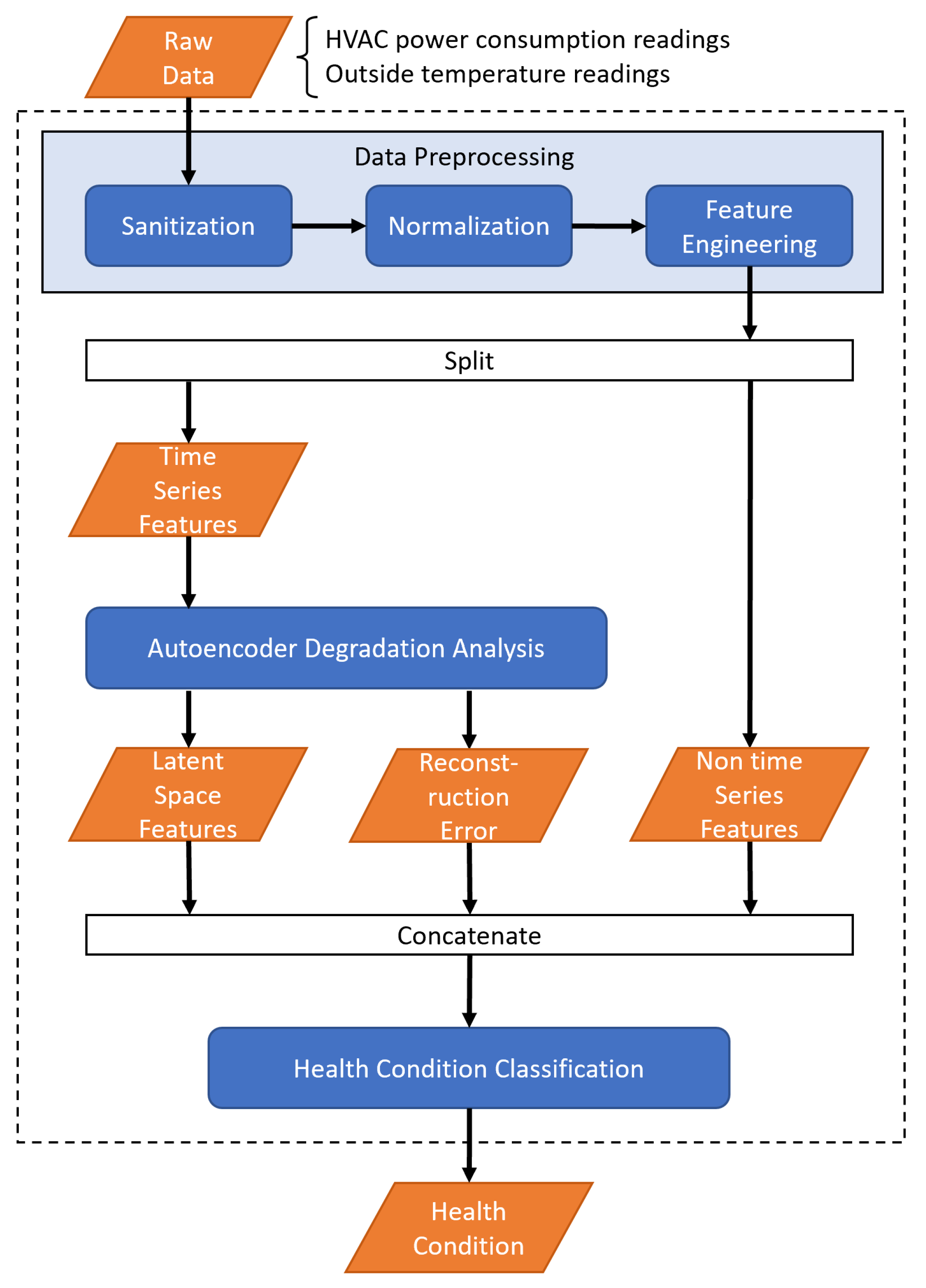
The HPC-AE framework, as illustrated in Figure 1, consists of three primary components: data preprocessing, autoencoder degradation analysis, and health condition classification. The data preprocessing component is responsible for data sanitation and feature engineering, which is crucial given the limited features associated with non-IoT-enabled HVAC systems. The intent is to derive a more comprehensive dataset for subsequent analysis.

The autoencoder degradation analysis component aims to distinguish between regular and degraded HVAC behaviors. Utilizing an autoencoder for this task is advantageous due to its aptitude to exhibit heightened reconstruction errors for degraded data samples as compared to regular samples. To refine the performance of the autoencoder, a multi-objective fitness function is introduced for hyperparameter optimization. The resultant latent space and reconstruction errors from the autoencoder further enhance the dataset.

Considering the dynamic operational patterns of HVAC systems—where an optimally functioning system might consume more power on a hot day compared to a malfunctioning one on a cooler day—it is imperative to note that the degradation analysis alone cannot yield accurate health classifications. Consequently, the health condition classification component takes on the task of the final health determination, employing a neural network-based multi-class classifier. Given the gradual nature of HVAC system degradation and the research’s emphasis on health prognostics, the HPC-AE framework analyzes daily HVAC power consumption to deduce daily health conditions.

As shown in Figure 1, the data preprocessing component refines the data, distinguishing between time series features such as power consumption and non-time series elements like daily minimums and maximums. Following this, the autoencoder degradation analysis component processes the time series features, yielding both a latent space representation and the associated reconstruction errors. Subsequently, these outputs are merged with the non-time series features and channeled into the health condition classification component, which deduces the daily health status of the HVAC system. The next subsections describe in detail the three major components of the framework: data preprocessing, autoencoder degradation analysis, and health condition classification.

3.1.1. Data Preprocessing

The first component in the proposed framework is the data preprocessing. This component is necessary to transform raw data into data suitable for machine learning models to train on. This component is further divided into three sub-components, namely data sanitization, normalization, and feature engineering. Data sanitization is needed because raw data often contain impurities which need to be removed. Normalization scales all data into the same range for machine learning algorithms to learn more effectively. Additionally, feature engineering contributes to building a richer dataset.

Data Sanitization

This framework incorporates a data sanitization process consisting of three crucial steps. Initially, to fix missing values commonly found in time series data like HVAC power consumption and external temperature, a missing data replacement step is used, where missing values are replaced with the mean of the neighboring valid observations. Second, a daylight savings time adjustment step is included to account for the one-hour shift observed in certain regions that could potentially skew the HVAC behavior data; this involves rolling back timestamps by one hour to align with local time and managing any discrepancies during daylight savings time transitions with the aforementioned missing data replacement strategy. Finally, the framework addresses regular inactivity periods in some HVAC systems, especially in commercial settings, where the systems are often set to a more energy-conserving mode or entirely shut down during off-peak hours. To ensure this inactivity does not affect the training process, an inactivity period removal step is applied to eliminate these periods from the dataset, thereby reducing the number of trainable parameters without negatively impacting the model’s performance. This last step, however, might not be necessary for residential HVAC systems due to variable occupation and usage patterns.

Normalization

Data normalization is critical in machine learning because features with a larger scale can overshadow those with a smaller scale, resulting in inferior performances. Min-max scaling (1) was applied to normalize the time series data because this scaler preserves the relationships among the input data [37].

$${x_i}^{\prime }=\frac{x_i-x_{min}}{x_{max}-x_{min}},$$

(1)

where $x_i$ is a value in the dataset, $x_{min}$ and $x_{max}$ are the minimum and maximum values of the dataset, and ${x_i}^{\prime }$ is the normalized value.

Feature Engineering

Feature engineering is crucial for the framework because it enriches the available features of the dataset. To engineer additional features from the time series data, the data are first grouped into daily windows such that the data in each window contain timestamps for one calendar day. Then, statistical features are calculated for each window, such as daily minimum, daily maximum, daily mean, and daily standard deviation for statistical features. In addition, date-related features are extracted based on the date of each window. This can include month of the year, day of the year, and day of the week. To preserve the periodical nature of date-related features, these features are encoded with trigonometric encoders using Equation (2).

$$\begin{array}{c}{x}_i^{sin}=sin\left(\frac{2\times \pi \times x_i}{\tau }\right),\\ x_i^{cos}=cos\left(\frac{2\times \pi \times x_i}{\tau }\right),\end{array}$$

(2)

where $x_i$ is a value in the dataset and $\tau$ is the period, e.g., 7 days in a week.

Lastly, the target classes were defined to determine the daily health condition of the HVAC system. In this work, three degradation classes are used to explain the methodology and conduct experiments. They are ND for no degradation condition, MD for moderate degradation condition, and SD for severe degradation condition. However, this framework is not restricted to work with only three health condition classes such that more classes may be considered. Figure 2 demonstrates the three target classes as well as the train, validation, and test set split of the dataset.

3.1.2. Autoencoder Degradation Analysis

The second component of the framework is the degradation analysis component. This component incorporates an autoencoder to differentiate between HVAC behaviors in normal and degraded conditions as well as generate additional features to aid the final classification of daily health conditions. In this component, an autoencoder is applied to the time series data in each daily window to analyze their relative degradation. As the autoencoder model is only trained with data samples without degradation, its parameters are optimized such that the reconstruction errors are minimized for normal operation behavior. Hence, the model would produce higher reconstruction errors for samples belonging to MD and SD classes. Once the autoencoder model is trained, the encoder will compress the input data into the latent space. Hence, both the reconstruction error and latent space features are used to generate an enriched dataset to be used in the health condition classification component.

3.1.3. Health Condition Classification

The health condition classification component is the last component of the HPC-AE framework. It is responsible for producing the final daily HVAC health conditions. In this component, a multi-class classification NN is used to classify the final daily health condition of an HVAC system. Specifically, the classifier used for this component is a multi-layer perceptron reproducing Thomas et al. [38] with an input layer, two hidden layers, and an output layer with three neurons, i.e., one output for each target class. The latent space and the reconstruction errors produced by the autoencoder and the non-time series features produced by the data preprocessing component are concatenated to form an enriched dataset for the classification task. This enriched dataset is used as the input to train the NN classifier.

Hyperparameter optimization for each classification model is conducted to ensure the best performance. The number of neurons in each hidden layer, the activation functions, and the learning rates are examples of hyperparameters that can be tuned for the NN classifier. The objective function for the hyperparameter optimization is the cross-entropy loss function. The classifier that yields the lowest cross-entropy loss value on the validation set across all tuned classifiers is selected as the final optimal classifier model.

3.2. Autoencoder Degradation Analysis Training Procedure

Because the autoencoder is used to generate an enriched dataset for the final health condition classification, the autoencoder hyperparameters are tuned so that the best-performing model is selected. Hence, the selection of the optimal autoencoder model is incorporated into autoencoder model training. This process adopts the exhaustive grid search strategy for model training and finds a list of candidate optimal autoencoder models based on their fitness scores. Hence, the autoencoder degradation training procedure is split into three steps: autoencoder model training, optimal model selection, and autoencoder feature generation, as shown in Figure 3. These steps are detailed in the following three subsections.

3.2.1. Autoencoder Model Training

The first step of the training process is autoencoder model training. In this step, the autoencoder model trains with all the sets of hyperparameter sets. Hyperparameters selected for the tuning process include the number of hidden layers, the number of neurons in each hidden layer, and the activation function [39]. An exhaustive grid search strategy is then used such that an autoencoder model is trained for each possible combination of the hyperparameter values. The autoencoder models are trained with the ND training set, while the ND validation set is used for early stopping of the training process to prevent model overfitting [40]. Fitness scores are calculated for these models to determine the list of candidate optimal models.

3.2.2. Optimal Model Selection

After all the autoencoder models are trained, a list of candidate optimal models is determined by the calculation of fitness scores. Conventionally for autoencoder hyperparameter optimization, the fitness of a model is usually determined using reconstruction errors [41,42]. However, in our scenario, minimizing the reconstruction error alone is not enough to determine the optimal model. To generate the best features for health condition classification, the autoencoder needs to not only minimize the reconstruction error for ND data samples but also distinguish between ND, MD, and SD samples in terms of the separation of reconstruction errors for each target class. Hence, a multi-objective optimization function is proposed to find the optimal model, with two objectives: $ob{j}_1$ and $ob{j}_2$.

The first objective is to minimize the reconstruction errors for the ND validation set. Specifically, the mean of reconstruction errors (3) is minimized.

$$ob{j}_1=\frac{1}{n}\sum _{i=1}^{n}R{E}_i^{ND}$$

(3)

where $RE$ is a vector of reconstruction errors evaluated in the ND validation set.

The second objective is to maximize the separation between the reconstruction errors for each of the classes. To calculate the separation of the reconstruction error, the mean logarithmic error (MLE) function is selected and is defined in (4). The MLE function is selected because it not only maintains the sign of the separations but also drastically reduces the effects of larger differences by the log transform, which in turn enhances the effects of smaller differences.

$$MLE(R{E}_1,R{E}_2)=\frac{1}{n}\sum _{i=1}^n({log}_e({R{E}_1}_i+1)-{log}_e({R{E}_2}_i+1)),$$

(4)

where $R{E}_1$ and $R{E}_2$ are vectors of the reconstruction errors. MLE applies natural log transformation to the two input vectors and then calculates the mean of the differences between the two transformed vectors.

The second objective is defined in (5), and determines the ability of the autoencoder to separate the three classes.

$$ob{j}_2=MLE(R{E}^{SD},R{E}^{MD})+MLE(R{E}^{MD},R{E}^{ND}),$$

(5)

Finally, the multi-objective function to be maximized with two objectives is defined by:

$$fitness=w_1|ob{j}_1|+w_2\left|ob{j}_2\right|,$$

(6)

where $w_1,w_2$ are weights for the objective functions, subject to $w_1+w_2=1$, and $w_1,w_2\in [0,1]$. $\left|·\right|$ is a min-max scaler used to normalize each objective function. In the calculation of the fitness score function, normalization is applied first to transform the objective functions such that they have the same order of magnitude [43]. Then, a weighted sum between the two objectives is calculated. By varying the parameters $w_1$ and $w_2$, the balance between the two objective functions varies. For each pair of weights considered, the autoencoder model that yields the highest fitness score is selected as a candidate optimal model.

3.2.3. Autoencoder Feature Generation

The final step in the autoencoder degradation analysis component is autoencoder feature generation. As discussed, the latent space features and the reconstruction errors are generated using the autoencoder model. These two features are concatenated with non-time series features produced by the data preprocessing component to form a new enriched dataset. This dataset is used for the final HVAC health condition classification. Because there are multiple candidate optimal autoencoder models, each candidate model is used to generate a new enriched dataset. Ultimately, all enriched datasets are passed to the health condition classification component for the final HVAC health condition classification.

4. Framework Evaluation

This section provides an extensive evaluation of the HPC-AE framework, where two case studies are conducted to evaluate the performance of HPC-AE against different HVAC fault scenarios. They are case study I (air filter clogging) and case study II (air duct leakage). This section begins with a description of the datasets utilized for this assessment, followed by an explanation of the chosen evaluation metrics. Thereafter, the setup for the experiment is presented in detail. For each case study, a series of four experiments were conducted, the results of which are subsequently analyzed. The initial experiment sets a performance benchmark using existing health prognostic methods in similar studies, while the following three experiments incorporate different autoencoders into the HPC-AE framework. The section culminates with a comparative performance analysis and a detailed discussion of the findings.

4.1. Synthetic Dataset Generation

To generate the datasets for framework evaluation, a building energy simulation software known as EnergyPlus (v22.2.0) [32] is utilized. EnergyPlus accepts a building model and a typical meteorological year (TMY) weather dataset as input and generates an assortment of sensor and meter readings as output, including the power consumption of the HVAC system installed in the building. In this work, an EnergyPlus-provided building template named “5ZoneAirCooled”, a popular template among researchers [44,45], is used for the simulations. (“5ZoneAirCooled” is packaged into the EnergyPlus installation. This template file can be found at $EnergyPlus installation$/ExampleFiles/5ZoneAirCooled.idf (accessed on 1 November 2022).) The “5ZoneAirCooled” template simulates a one-story building which houses a standard variable air volume (VAV) system. Heating is achieved via a single boiler and hot water reheat coil, while cooling is achieved via an electric compression chiller with an air-cooled condenser and chilled water coil. For the purpose of simulating an HVAC system in degraded conditions, i.e., to generate power consumption data in MD and SD conditions, the “5ZoneAirCooled” template is modified with the inclusion of the EnergyPlus fault model [46], which allows for the injection of certain types of faults into the HVAC system. Furthermore, the TMY weather data collected at Lester B. Pearson International Airport (the TMY weather datasets used for this work are available at OneBuilding.Org (accessed on 15 January 2023).), located in Toronto, Canada, are used as weather input to run the simulations.

4.1.1. Clogged Air Filter

In the clogged air filter scenario, data are generated using the EnergyPlus air filter fault model to simulate the impact of a dirty air filter on the VAV supply fan. A study by Nassif [36] indicated that moderately dirty air filters can lead to an average 14.3% increase in annual HVAC power consumption, with a significant increase of 28.4% for heavily soiled filters. Using these insights, the fault intensity parameter in the model is adjusted to mirror a simulated annual HVAC power consumption increase of 14.3% for the MD condition and 28.2% for the SD condition compared to normal operation. The resultant data, illustrating HVAC power consumption variations for the three conditions, is presented in Figure 4a.

4.1.2. Leaking Air Ducts

In the air duct leakage scenario, the study utilized a simplified duct leakage model to generate data, simulating the consequences of an air duct experiencing leaks. Research by Yang et al. [47] highlighted that approximately 40% of the analyzed HVAC rooftop units exhibited airflow-related issues. Building on insights from Tun et al. [48], which outlined multiple HVAC system faults, this study replicates the air duct leakage fault at both 10% and 20%. Specifically, an upstream and downstream nominal leakage fraction of 0.1 is employed to generate HVAC power consumption data for the MD condition, while a leakage fraction of 0.2 is designated for the SD condition. Figure 4b shows the data generated for the comparison of the HVAC power consumption in ND, MD, and SD conditions in this scenario.

Overall, a total of six weather datasets are used to simulate the HVAC power consumption (six rows in Figure 5). For each weather dataset, the HVAC power consumption for ND, MD, and SD conditions are simulated (three columns in Figure 5). The data resolution is set to a quarter-hour. Thus, each day contains 96 readings of the two features. The HVAC simulations are run for the period from 1 May to 31 October, for a total of 184 days. Consequently, the final synthetic dataset contains 3312 daily samples, i.e., 184 days × 3 conditions × 6 simulations. Data generated by all six simulations in the ND condition are assigned with the no degradation label. The same is true for data generated in the two degraded conditions. Hence, this dataset is a balanced dataset, as each health condition contains the same number of simulated days.

The dataset is then split into training, validation, and testing sets. Figure 5 illustrates this split. First, the synthetic data generated by one of the TMY datasets (Simulation 6 in Figure 5) are set aside and reserved for testing the models’ generalization performance. Then, for the remaining five simulations for the ND, MD, and SD conditions, which account for 2760 samples, the dataset is split into 80% and 20% for training and validation sets. In consequence, there are 2208 samples in the training set, 552 samples in the validation set, and another 552 in the testing set. Dedicating an entire simulation for testing is beneficial because an entire simulation contains HVAC data for each day from May to October for each health condition, which covers a wider range of weather conditions and HVAC power consumption trends.

4.2. Evaluation Metrics

To evaluate the model performance, the multi-class F1 score and the area under the receiver operating characteristics curve (AUROC) were used. The computation of the F1 score necessitates the prior calculation of two metrics, precision and recall, as defined by (7) and (8), respectively. Precision epitomizes the ratio of correctly classified positive samples to the total predicted positive samples. In contrast, recall quantifies the proportion of accurately identified positive samples out of the total actual positive samples.

$$Precision=\frac{TP}{TP+FP}$$

(7)

$$Recall=\frac{TP}{TP+FN}$$

(8)

F1 score is a popular accuracy measure for machine learning models. It is defined as the harmonic mean of precision and recall. The equation to calculate the F1 score is given by (9). A higher 1 score indicates a higher model performance. An F1 score of 1 represents a model that can correctly classify all instances. In this work, the macro-averaging method is used to calculate the F1 score in a multi-class setting. The macro-averaged F1 score is the unweighted average of the F1 score for each individual class, and it is given by (10).

$$F_1=2\frac{Precision·Recall}{Precision+Recall}$$

(9)

$$F_1^{macro}=\frac{1}{n}\sum _{i=1}^n{F}_1^{C_i}$$

(10)

where n is the number of classes to be classified and $F_1^{C_i}$ is the F1 score calculated for the i-th class.

The area under the receiver operating characteristic (AUROC) provides a visual representation of a binary classifier’s performance with varying decision thresholds. In an ROC curve, the true positive rates (TPR) evaluated at varying thresholds are plotted against the false positive rates (FPR). The TPR is the same as recall. The FPR is the proportion of actual negative samples which are misclassified as positive. The ROC curve has both a domain and a range of [0, 1]. For a model that classifies no better than random chance, the ROC curve resembles a diagonal line from coordinates (0, 0) to (1, 1). On the other hand, for a perfect classifier, the ROC curve follows the y-axis from (0, 0) to (0, 1), then a horizontal line from (0, 1) to (1, 1).

4.3. Experiments Setup

The experiments were conducted on a desktop PC equipped with an Intel Core i7-9700k CPU, an NVIDIA GeForce RTX 2080 GPU, and 32 GB DDR4 memory. Python 3.9 was employed, utilizing the Tensorflow 2.6.0 library with the Keras API. The baseline models were developed using the Sci-kit Learn 1.2.1 library. GPU acceleration, facilitated by the cuDNN 8.2.1 library, was leveraged for training the long short-term memory (LSTM) neural network models. Dataset manipulation was accomplished using Pandas 1.5.2 and Numpy 1.23.5 libraries, while the Matplotlib 3.5.3 library aided in generating the result figures.

To ensure fairness across all experiments, the same data are used for training all three baseline models as well as the HPC-AE framework with the three different autoencoders. The dataset is prepared using the data preprocessing component in the HPC-AE framework. Recall that the electric meter readings have a 15 min resolution. In consequence, each day contains a total of 96 readings. The daily HVAC power consumption and outside temperature readings from midnight to 6 A.M. (24 readings) are removed because of inactivity, which reduces the number of readings from 96 to 72 per day. Statistical and time-derived features are calculated following the feature engineering step in the data preprocessing component. After data preprocessing, the dataset contains a total of 158 features per day. All machine learning algorithms are trained with three different seeds.

4.4. Experiments Process

This subsection details the procedure adopted for each experimental evaluation. To assess the efficacy of the HPC-AE framework, four distinct experiments were conducted for each study case. In the first experiment, existing methods for HVAC health prognostics are evaluated to establish a baseline performance. Three methods are considered: multi-layer perceptron classifier (MLP-C), support vector machine (SVM), and decision tree (DT). In the three subsequent experiments, the proposed framework is evaluated with the use of three different autoencoder methods, namely dense autoencoder (DAE), convolutional autoencoder (CAE), and long short-term memory autoencoder (LSTMAE). In experiment II with DAE, the objective is to study the effect of the inclusion of a simple autoencoder over directly using a classifier for HVAC health condition classification. In experiments III and IV with CAE and LSTMAE, the objective is to study the performance gain when using autoencoders with more complex architectures.

4.4.1. Experiment I: Performance Baseline

In the first experiment, existing health prognostic methods for HVAC systems [12,23] are evaluated on the dataset from both case studies. Three machine learning models are considered for the baseline comparison: multi-layer perceptron classifier (MLP-C) [23], support vector machine (SVM) [23], and decision tree (DT) [12]. The objective of this experiment is to investigate the performance of existing methods in a scenario where the number of features is limited.

Table 1. Hyperparameters used for the baseline models.

Baseline	Hyperparameter	Values for Case
		Study I	Study II
MLP-C	hidden layers	2	2
	hidden units	474	316
	optimizer	Adam	Adam
	activation function	Sigmoid	Tanh
	learning rate	0.01	0.0001
SVM	l2 regularization	53.37	1000
	kernel function	RBF	RBF
DT	criterion	GINI	GINI
	max depth	10	10
	max features	sqrt	sqrt
	min split	2	2
	min leaf	4	9

shows the optimal hyperparameters chosen for each baseline model. These values are determined after employing the exhaustive grid search method across three distinct seeds. The outcomes from these three models serve as the foundational performance benchmark.

4.4.2. Experiment II: Health Prognostics Classification with Dense Autoencoder (HPC-DAE)

HPC-AE uses the autoencoder component to extract features from the daily HVAC data before classifying the health condition of the system. In this experiment, the HPC-AE is evaluated with a dense autoencoder (DAE) for the autoencoder degradation analysis component. The goal of this experiment is to study the effect of using a simple autoencoder for feature generation. First, the exhaustive grid search technique is applied to train a collection of autoencoders with the ND training set. Their fitness scores are then calculated using the ND, MD, and SD validation set by applying (6). For each $w_1$ and $w_2$ pair, the hyperparameters that yield the highest fitness score are presented in

Table 2. Hyperparameters for the DAE candidates for each case study.

Case	Candidate	[w1, w2]	Topology *	Activation	lr	Dropout	CE Loss
Study I	1	[0, 1]	(54, 27)	ReLU	0.0001	0	0.3012
	2	[0.25, 0.75]
	3	[0.5, 0.5]	(36, 27)	Sigmoid	0.01	0.1	0.3260
	4	[0.75, 0.25]	(36, 27)	Sigmoid	0.0001	0	0.3479
	5	[1, 0]	(72, 54)	Tanh	0.001	0	0.3854
Study II	1	[0, 1]	(27, -)	ReLU	0.0001	0	0.3253
	2	[0.25, 0.75]
	3	[0.5, 0.5]	(54, 36)	Sigmoid	0.01	0	0.3618
	4	[0.75, 0.25]	(72, 36)	Tanh	0.01	0.1	0.3856
	5	[1, 0]	(72, 54)	Tanh	0.001	0	0.3698

* Topology: two hidden layers of neurons for encoder and decoder. Number of neurons for each layer.

; they are also referred to as candidates. Each candidate represents a collection of three trained autoencoders given three trials with different seeds. Because candidates 1 and 2 have the same hyperparameters, results and hyperparameters for candidates 1 and 2 are merged. The autoencoders which are trained using the optimal hyperparameters are then used to generate the enriched dataset for health condition classification NN training.

The last column of Table 2 shows the classification loss function performance for each HPC-DAE candidate. The loss function used is the average cross-entropy (CE) calculated against the validation dataset. For the CE loss, the lower the value, the better. The candidate with the best CE results is shown in bold. Based on the CE results, the best HPC-DAE models for both case studies are candidate 1, with a validation loss of 0.3012 and 0.3253 for case studies I and II, respectively. Then, candidate 1 models are used for calculating HPC-DAE performance against the test set.

4.4.3. Experiment III: Health Prognostics Classification with Convolutional Autoencoder (HPC-CAE)

In this experiment, the HPC-AE is evaluated with a convolutional autoencoder (CAE) for the autoencoder degradation analysis component. The goal of this experiment is to study how much the classification performance can be improved by using a more complex autoencoder over a simple DAE. A convolutional autoencoder also specializes in extracting temporal relationships within time series features. The same steps taken in experiment II to train and select the model are reproduced in this experiment.

Table 3. Hyperparameters for the CAE candidates for each case study.

Case	Candidate	[w1, w2]	Latent	Kernel	Activation	lr	CE Loss
Study I	1	[0, 1]	54	9	ReLU	0.01	0.3044
	2	[0.25, 0.75]
	3	[0.5, 0.5]	72	5	Tanh	0.01	0.3648
	4	[0.75, 0.25]	54	7	Tanh	0.01	0.4022
	5	[1, 0]	36	3	Tanh	0.01	0.3904
Study II	1	[0, 1]	27	3	Sigmoid	0.01	0.3390
	2	[0.25, 0.75]
	3	[0.5, 0.5]
	4	[0.75, 0.25]	72	5	Tanh	0.01	0.3932
	5	[1, 0]	54	9	Tanh	0.001	0.3898

shows the best CAE component for each pair of fitness score weights parameters $w_1$ and $w_2$. Each candidate represents a collection of three trained autoencoders given the use of three seeds. For case study I, because candidates 1 and 2 share the same set of optimal hyperparameters, they are merged together. For case study 3, candidates 1, 2, and 3 are merged together.

Table 3 shows the average cross-entropy (CE) for each candidate, calculated against the validation dataset. For the CE loss, the lower the value, the better. The candidate with the best CE results is shown in bold. Based on the CE results, the best HPC-CAE model is candidate 1, with a validation loss of 0.3044 and 0.3390 for case studies I and II, respectively. Then, candidate 1 models are used for calculating HPC-CAE performance against the test set.

4.4.4. Experiment IV: Health Prognostics Classification with Long-Short Memory Autoencoder (HPC-LSTMAE)

In the last experiment, the use of a long short-term memory autoencoder (LSTMAE) is evaluated for the autoencoder degradation analysis component. This experiment aims to assess the efficacy of the framework when integrating an autoencoder specialized for time series. The same steps from experiment II to train and select the model are reproduced in this experiment.

Table 4. Hyperparameters for the LSTM candidates.

Case	Candidate	[w1, w2]	Topology *	Early Stop	Dropout	CE Loss
Study I	1	[0, 1]	(72, 54)	0.01	0.2	0.3036
	2	[0.25, 0.75]
	3	[0.5, 0.5]
	4	[0.75, 0.25]	(72, 54)	0.001	0	0.3663
	5	[1, 0]
Study II	1	[0, 1]	(54, -)	0.01	0	0.3399
	2	[0.25, 0.75]
	3	[0.5, 0.5]
	4	[0.75, 0.25]
	5	[1, 0]	(54, -)	0.0001	0	0.4193

* Topology: two hidden layers of neurons for encoder and decoder. Number of neurons for each layer.

shows the best LSTMAE component for each pair of fitness score weights parameters $w_1$ and $w_2$. Each candidate represents a collection of three trained autoencoders given the use of three seeds. Note that for HPC-LSTMAE, candidates 1, 2, and 3 share the same optimal hyperparameters, while candidates 4 and 5 share another set of optimal hyperparameters. After merging, only two candidates are used for the health index indicator calculation.

Table 4 shows the average CE for each candidate, calculated against the validation set. Based on the CE results, the best HPC-LSTMAE model is candidate 1, with a validation loss of 0.3036 and 0.3399 for case studies I and II, respectively. Then, candidate 1 models are used for calculating HPC-LSTMAE performance against the test set.

4.5. Experiment Results

This subsection delineates the outcomes obtained from each experimental case study. Results corresponding to the clogged air filter scenario are first discussed, followed by findings related to the leaking air ducts scenario.

4.5.1. Results for Case Study I: Clogged Air Filter

In this study case, data were produced to mimic the impact of a dirty air filter on a VAV supply fan, utilizing the air filter fault model from EnergyPlus. The dataset was structured to reflect both normal operation and degraded conditions as detailed in Section 4.1.1. Subsequently, methodologies from experiments 1 through 4 were applied to this specific dataset. The optimal models were then employed to compute outcomes on the test set, with F1 and AUROC scores being averaged over three trials, each with distinct seeds.

The results for the baseline models and the HPC-AE framework with the three autoencoders methods are shown in

Table 5. Classification performance results for the clogged air filter case study.

Method	F1 Score	AUROC Score	Improvement over MLP-C
			F1 Score	AUROC
DT	0.7654	0.9111	−5.40%	−4.44%
SVM	0.8005	0.9422	−1.06%	−1.17%
MLP-C	0.8091	0.9534	-	-
HPC-DAE	0.8463	0.9644	4.60%	1.36%
HPC-CAE	0.8555	0.9746	5.73%	2.22%
HPC-LSTMAE	0.9533	0.9725	5.46%	2.00%

. F1 scores and AUROC scores exhibited by the three baseline models show that they are not as good at achieving a balance between precision and recall. Based on the baseline results, the MLP-C is the best-performing baseline model, with an F1 score of 0.8091 and an AUROC of 0.9534. It is then used for comparison against the HPC-AE variants.

The F1 scores for the three autoencoder methods within the HPC-AE framework are also detailed in Table 5. The method with the best results is shown in bold. HPC-DAE shows a 4.60% improvement in the F1 score compared to the baseline MLP-C model. HPC-CAE records an F1 score of 0.8555, marking a 5.73% improvement over the baseline. Additionally, HPC-CAE’s performance slightly surpasses that of HPC-DAE, suggesting that a more intricate autoencoder structure might be advantageous for the HPC-AE framework. On a similar note, HPC-LSTMAE outperforms the baseline MLP-C model in classifying ND and MD instances with an average F1 score of 0.8533. Its performance is slightly better than HPC-DAE and closely matches HPC-CAE.

4.5.2. Results for Case Study II: Leaking Air Ducts

In this study case, data was formulated using a simplified duct leakage model to capture the implications of leakages in an air duct in a model from EnergyPlus. The dataset was structured to reflect both normal operation and degraded conditions, as detailed in Section 4.1.2. Subsequently, methodologies from experiments 1 through 4 were applied to this specific dataset. The optimal models were then employed to compute outcomes on the test set, with F1 and AUROC scores being averaged over three trials, each with distinct seeds.

Performance results for the baseline models, along with the HPC-AE framework, are presented in

Table 6. Classification performance results for leaking air ducts case study.

Method	F1 Score	AUROC Score	Improvement over MLP-C
			F1 Score	AUROC
DT	0.6659	0.8567	−17.24%	−8.61%
SVM	0.8022	0.9308	−0.30%	−0.70%
MLP-C	0.8046	0.9374	-	-
HPC-DAE	0.8209	0.9473	2.03%	1.06%
HPC-CAE	0.8005	0.9464	−0.50%	0.97%
HPC-LSTMAE	0.8213	0.9521	2.08%	1.58%

. Compared to Table 5, which presents baseline performance for case study I, the performances of all three baseline models show a slight decrease in F1 and AUROC scores. This suggests that it could be harder to detect a leak in the air ducts of an HVAC system than a clogged air filter. Nonetheless, the baseline MLP-C method still outperforms SVM and DT methods to be the best baseline method, yielding an average F1 score of 0.8046 and an average AUROC score of 0.9374. It is then used for comparison against the HPC-AE variants.

The F1 scores for the three autoencoder methods within the HPC-AE framework are detailed in Table 6. The method with the best results is shown in bold. The HPC-DAE method registers an F1 score of 0.8209, marking a 2.03% improvement. HPC-CAE, while optimal in the clogged air filter scenario, shows a slight decrease in its F1 score for the air duct leakage scenario, suggesting challenges in information extraction. Conversely, HPC-LSTMAE displays a 2.08% improvement in its F1 score over the baseline MLP-C method, highlighting its consistent efficacy and suggesting its suitability within the HPC-AE framework.

5. Discussion

To analyze the effectiveness of the proposed HPC-AE framework, the framework is evaluated in two HVAC fault scenarios including a clogged air filter and leaking air ducts. Furthermore, the performance of HPC-AE is compared to that of machine learning methods in related studies that also focus on HVAC health prognostics. As described in experiment I, three baseline models, which include MLP-C, SVM, and DT, are considered for performance comparison based on similar studies by Cheng et al. [23] and Yang et al. [12]. Although both studies also focus on HVAC health prognostics, the method by Cheng et al. [23] finds a number between 0 and 10 as the health indicator and the method by Yang et al. [12] finds the remaining useful life in number of days, whereas the HPC-AE framework presented in this study considers three classes for health condition classification. Hence, the results from the three studies cannot be directly compared. Consequently, the machine learning models used in both studies are applied to the dataset in this experiment to establish a baseline performance which the HPC-AE framework is compared against.

The performance results of the HPC-AE framework in comparison with the baseline method are depicted in Figure 6. These results display scores from three trials for two HVAC fault scenarios: a clogged air filter and air duct leakage. The outcomes indicate that the HPC-AE framework, incorporating three autoencoder methods, either surpasses or closely matches the performance of the baseline methods. A closer comparison among the autoencoder methods reveals that the LSTMAE method offers superior performance across both fault scenarios, attributed to its minimal variance and elevated F1 score relative to the CAE and DAE methods. While the CAE method demonstrates commendable performance in the clogged filter scenario, it lags behind in the leaking duct situation. Thus, the LSTM autoencoder emerges as the most optimal choice for the HPC-AE framework.

The overall performance of the HPC-AE framework demonstrates that it is a promising approach for HVAC health prognostics with HVAC power consumption and outside temperature data. Nonetheless, the HPC-AE framework is not without limitations. Some potential limitations of the framework are as follows:

• The HPC-AE framework classifies the health condition by detecting the increase in power consumption of a degraded HVAC system. This means that the framework is only sufficient for the degradation of electrical or mechanical components in HVAC systems that tend to increase their power consumption.
• The HPC-AE framework frames HVAC health prognostics into a multi-class classification task, and its performance is evaluated on a synthetic dataset with three predetermined levels of health conditions. However, in a real-world scenario, the degradation of an HVAC system would likely be more gradual. Hence, the framework may struggle to correctly classify the HVAC system’s health condition when the input features fall near a decision boundary. For instance, when the condition of an HVAC system has started to deteriorate but not quite to the level of moderate degradation, HPC-AE’s prediction may fluctuate between no degradation and moderate degradation for a duration of time.
• This framework does not consider other factors that may affect HVAC power consumption in addition to the outside temperature, e.g., the building occupancy information, because the collection of these data is not as easy. This means that the framework may not perform as well in situations where the building occupancy level can fluctuate by a large amount. In situations where the presence of human activity in the building is higher than normal, the HVAC system would likely consume more power to cool off the additional heat. This can cause HPC-AE to falsely classify the HVAC system as more degraded and vice versa.

6. Conclusions

This study introduces the health prognostics classification with autoencoders (HPC-AE) framework, a distinctive data-driven HVAC predictive maintenance system that categorizes HVAC health into distinct levels based on daily power consumption and external temperature patterns. The HPC-AE framework integrates an autoencoder, which derives a generalized representation from time series data, enabling reconstruction errors to reflect the relative degradation of data samples. To optimize the autoencoder’s performance, an exhaustive grid search is employed, evaluating various hyperparameter combinations. Subsequently, a multi-objective fitness score aids in identifying the optimal autoencoder model, aiming to minimize reconstruction errors for the no degradation state while distinguishing errors for all three health conditions. Once the optimal autoencoder is selected, a new enriched dataset is formed using the outputs from the autoencoder for the final daily HVAC health condition classification.

The HPC-AE framework is evaluated with the use of three different types of autoencoders, namely, the dense autoencoder (DAE), convolutional autoencoder (CAE), and long short-term memory autoencoder (LSTMAE), with two fault scenarios. The DAE is the simplest form of autoencoder, whereas the CAE and LSTMAE have more complex structures that allow both to extract temporal features from the input data. The efficacy of these methods is benchmarked against existing machine learning techniques in HVAC health prognostics literature, including MLP-C, SVM, and DT, all assessed using an identical dataset. The HPC-AE method outperforms the best baseline model, MLP-C, by an increase of 5.73% and 2.22% in F1 and AUROC score in the clogged air filter scenario and an increase of 2.08% and 1.58% in the leaking air ducts scenario. Within three HPC-AE variants, HPC-LSTMAE demonstrates high performance in both HVAC fault scenarios thanks to their better generalization abilities.

As discussed previously, the HPC-AE framework is limited in that it can only be applied to types of HVAC degradation that result in an increase in its power consumption. Additionally, a multi-class approach to determining the equipment’s health conditions may cause misclassification near decision boundaries. Lastly, factors such as building occupancy are not considered due to the added difficulty of collection, which may reduce the classification performance.

Future research will focus on enhancing the framework’s classification accuracy and providing additional validation. Exploring different types of autoencoders, such as the variational autoencoder, known for its efficacy in fault detection, might improve the framework’s performance. Additionally, the incorporation of contrastive representation learning might improve the autoencoder’s capacity to differentiate between normal and different degraded states. For further validation of the framework, one possible direction is to investigate how the parameters of the EnergyPlus fault model may vary gradually over time such that more realistic degradation behaviors of HVAC systems could be simulated. Furthermore, this work validates the HPC-AE framework in two HVAC degradation scenarios including a clogged air filter and leaking air ducts. Although the framework demonstrates its proficiency in these two scenarios, more HVAC degradation scenarios are to be experimented with for more definitive proof.