Abstract
With the fast increase of solar energy plants, a high-quality short-term forecast is required to smoothly integrate their production in the electricity grids. Usually, forecasting systems predict the future solar energy as a continuous variable. But for particular applications, such as concentrated solar plants with tracking devices, the operator needs to anticipate the achievement of a solar irradiance threshold to start or stop their system. In this case, binary forecasts are more relevant. Moreover, while most forecasting systems are deterministic, the probabilistic approach provides additional information about their inherent uncertainty that is essential for decision-making. The objective of this work is to propose a methodology to generate probabilistic solar forecasts as a binary event for very short-term horizons between 1 and 30 min. Among the various techniques developed to predict the solar potential for the next few minutes, sky imagery is one of the most promising. Therefore, we propose in this work to combine a state-of-the-art model based on a sky camera and a discrete choice model to predict the probability of an irradiance threshold suitable for plant operators. Two well-known parametric discrete choice models, logit and probit models, and a machine learning technique, random forest, were tested to post-process the deterministic forecast derived from sky images. All three models significantly improve the quality of the original deterministic forecast. However, random forest gives the best results and especially provides reliable probability predictions.
1. Introduction
Solving the challenges posed by the massive integration of solar energy into electricity grids is a key issue for reducing the carbon footprint of power generation. Indeed, due to the inherent variability and lack of predictability of solar energy, a high share of solar energy in the electricity mix makes it more complicated to manage the supply-demand balance and increases the vulnerability of the grid. One of the strategies to reduce the effect of solar variability is to predict future solar irradiance and corresponding solar power for short-term horizons ranging from 1 min to several days in advance. Many techniques have been developed to predict solar irradiance [1,2,3]. Numerical weather prediction (NWP) is suitable for horizons longer than 6 h. Forecasts derived from geostationary meteorological satellite images are effective for a horizon ranging from about 1 h to 6 h. It is also important to consider the target application to provide relevant forecasts. For instance, for common PV plants, one should forecast the global solar irradiance in the plane of the array, which includes both direct and diffuse components [3]. For the particular case of CSP plants, which have a narrow view angle facing the sun [4], reliable forecasts of the beam’s normal irradiance are required. Therefore, to forecast the solar energy for CSP plants and for very short-term horizons of less than 1 h, the approach based on all sky imagers (ASI) seems to be a promising technique [5,6].
Regarding the very short-term horizon, Ajith and Martínez-Ramón [7] compared three categories of solar irradiance forecasting methods: time series, sky camera images, and hybrid models combining infrared images with radiation time series. The authors showed that the normalized root mean square error (nRMSE) varied from 30 to 53% in terms of forecasting error. In the literature on ASI, most of the works dealing with the prediction of solar irradiance or cloudiness propose deterministic forecasts [8,9,10]. To improve forecasts derived from ASI, different approaches have been carried out. For instance, Paletta et al. [11] evaluated deterministic and probabilistic predictions based on ASI for different weather conditions (clear, cloudy, and overcast skies). In their work, the probabilistic approach demonstrates a richer operational forecasting framework by facilitating uncertainty quantification in cloudy conditions and for long-term horizons. With the same aim, Nouri et al. [12] used a statistical analysis of historical data to add uncertainty to ASI deterministic forecasts. Their original approach allows the creating of a probabilistic forecast of the DNI and GHI. However, very few recent methods were developed to generate probabilistic forecasts from sky camera images.
It is well-known that weather forecasts are uncertain because the evolution of the weather and consequently solar irradiance are chaotic processes. Thus, in decision-making operations that use solar forecasts, such as the management of power plants, probabilistic forecasts are crucial. Indeed, probabilistic forecasts assign probability levels to future events and allow their users to assess the associated risks. Research works dealing with probabilistic solar forecasts are relatively recent but numerous works have been released on the topic in the last 10 years [3,13,14]. However, as mentioned previously, very few works concerning ASI proposed a method to generate a probabilistic solar forecast. This work will contribute to filling this gap in the literature.
Usually, solar forecasting systems provide the future level of solar irradiance or PV generation as a continuous variable [3]. But, for particular applications, such as the management of concentrated solar plants (CSP) with tracking devices, the operator needs to anticipate the achievement of a solar irradiance threshold to start or to stop their system [15]. In this case, an accurate binary forecast is more relevant. In the wide domains of meteorology or economy, numerous works propose discrete choice models to generate binary forecasts [16,17]. However, in the field of solar energy, very few works propose binary forecasts. One of the rare works on the topic is proposed by Alonso and Batlles [18] who developed a method to forecast the cloudiness from a sequence of images given by the MeteoSat Second Generation (MSG) satellite MSG or an ASI. Their model generates deterministic binary forecasts of cloud presence (i.e., cloudy and clear sky) corresponding to a direct normal irradiance (DNI) above 400 W/m. The forecasts were tested over 2 years for the city of Almería in the south-east of Spain. The success rate of the forecasts derived from the ASI is 83% for the first 15 min and drops to 60% for a 3 h horizon. However, no work proposes a probabilistic approach to generate discrete solar forecasts. Indeed, the probabilistic approaches developed previously in the field of solar energy derive an irradiance level, also called quantile, from a fixed probability. As a consequence, they do not allow estimating the probability of reaching an arbitrary chosen irradiance threshold. Therefore, the main challenge of this work is to propose a methodology and suitable models able to precisely forecast the probability of crossing a defined irradiance level.
In light of the two main lacks of the literature underlined above, the main objective of this work is to propose a novel methodology to generate probabilistic solar forecast as a binary event for horizons ranging from 1 to 30 min using an all sky imager. The developed approach will combine a state-of-the-art ASI method and discrete choice models proposed in other domains, such as economy or meteorology. In a first step, a model based on the detection of cloud motions will use sequences of images from an ASI to generate binary deterministic forecasts of the cloudiness. This deterministic prediction is focused on the operation of concentrating solar thermal power plants, mainly central tower plants, since the appearance of clouds is a conditioning factor that can affect the operation and integrity of different components of the facilities, such as the central receivers [19]. Then, in a second step, binary choice models will be used to convert the deterministic discrete forecasts into probability levels of cloud presence. Finally, we will assess the quality of the generated forecasts on a case study to evaluate the added value of the proposed method.
The remainder of the paper is organized as follows. Section 2 presents the methodology used to develop and evaluate the proposed model. Section 3 gives a brief overview of the state-of-the-art model used to generate the deterministic forecasts. Then, Section 4 details the discrete choice models used to forecast the probability of cloud presence. Section 5 depicts the case study and the corresponding data. Results are presented and discussed in Section 6. Finally, Section 7 gives our concluding remarks.
2. Overall Methodology and Forecasts Evaluation
The probabilistic forecasts are generated in two steps as presented in Figure 1. First, we generated deterministic forecasts of cloud presence using the method proposed by [18] and briefly presented in Section 3. The results are discrete forecasts (1 = no cloud and 0 = presence of clouds) with a time resolution of 1 min and horizons of forecast up to 30 min. The second step is a post-processing of the deterministic forecasts with a probabilistic model. In this work, we compared three different models, described in Section 4, to post-process the deterministic forecasts. The final probabilistic forecasts have the same temporal resolution and the same horizons as the deterministic forecasts. After these two steps, the generated forecasts are probabilities, in the interval , that gives a level of confidence or risk associated with the future presence of clouds. Compared to deterministic forecasts, this additional information may help the user in decision-making.
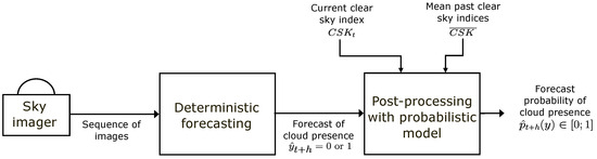
Figure 1.
Diagram of the implementation of the forecasting models at time t and a horizon of forecast h.
To evaluate the forecasts done with the methodology described above, we propose to use a simple concept of detection of clouds that mask the sun based on DNI measurements and CSP operation. Thus, cloud detection was carried out following the methodology presented in [20] obtaining a cloud identification (clouds which attenuate the DNI below 400 Wm) based on the optimal operating value for CSP plants, as the case of the Gemasolar plant, which used this irradiance level, like the appropriate for producing electricity [18].
In this work, both deterministic and probabilistic forecasts will be evaluated. If comprehensive frameworks have been proposed to evaluate forecast quality of the solar irradiance as a continuous variable [21,22,23], no previous work details the evaluation of discrete solar forecasts. However, specific error metrics have been designed in the field of meteorology to assess the quality of binary forecasts. Let us recall that the quality of a forecasting system evaluates the agreement between the forecasts and the corresponding observations [24]. Interested readers may refer to the web page published by the Joint Working Group on Forecast Verification Research to have an extended overview of weather forecast verification [25].
Regarding binary deterministic forecasts, the most common metrics are derived from the confusion matrix presented in Figure 2. In our case, a “yes” event corresponds to a clear sky (no clouds) and N is the total number of observation/forecast pairs used for the verification. The confusion matrix is a useful tool for classifying the types of errors. A perfect forecast system would generate only hits and correct negatives, and no misses or false alarms. Numerous metrics are derived from the four cells in the confusion matrix, such as fraction correct, probability of detection (POD) or its opposite probability of false detection (PODF), success rate (SR), or false alarm ratio (FAR) [26]. Each metric describes a different aspect of forecast performance. In this work we will focus on the accuracy, defined in Equation (1). Accuracy ranges from 0 to 1, with 1 the perfect score. The accuracy also called fraction correct gives the fraction of correct forecasts. It is simple and intuitive but, in case of very rare events, this indicator may lead to confusion [25].
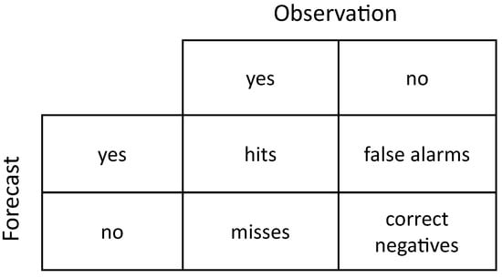
Figure 2.
Confusion matrix for a binary forecast.
Regarding the verification of probabilistic forecasts, two main attributes define the quality: the reliability and the resolution. Reliability refers to the statistical consistency between the forecasts and the observations. In other words, the forecast probability should be equal to the observed probability of the event (e.g., 20% of the events should happen for a forecast probability of 20%). The reliability is a crucial prerequisite as non-reliable forecasts would lead to a systematic bias in subsequent decision-making processes [27]. The most used visual tool to assess reliability is the reliability diagram [28]. Resolution refers to the ability of a forecasting system to generate case-dependent forecasts. For example, the climatology model, which predicts the average probability of the event (i.e., always the same probability regardless of the horizon or the weather conditions) has no resolution. Similarly to the reliability diagram, the ROC (relative operating characteristic) diagram [29] provides a visual assessment of the resolution. It plots the hit rate (Equation (2)) against the false alarm rate (Equation (3)), for a set of increasing probabilities (e.g., 0.1, 0.2, 0.3, etc.). It is a measure of the ability of the forecasting system to discriminate between two different outcomes.
Only a few metrics, also called scores, exist to quantitatively evaluate the quality of probabilistic forecasts of binary events. For this work, we propose to use the Brier Score (BS) [24], formulated as follows:
where N is the number of observation/forecast pairs, the forecast probability, and the observation. If the event did occur , and if it did not occur . The BS measures the mean square probability error. This global proper score is appealing because it includes the two basic skills of a probabilistic forecast (i.e., reliability and resolution) and it corresponds to for a deterministic forecast. The BS ranges between 0 and 1 with 0 the perfect score.
Skill scores (SS), derived from the above-mentioned metrics are also commonly proposed to evaluate forecast quality [21,22]. SS quantify the improvement of a proposed method compared to a reference model. They are relevant for comparing forecasts generated for different sites or time periods. In this work, we will compute a SS based on the BS with the climatology as a reference, as given in the following equation:
3. Deterministic Forecasts of Cloud Presence with a Sky Camera
To issue a forecast, a sequence of consecutive sky camera images is required. Following the methodology proposed by [18], three consecutive images are enough to make a prediction. The next step consists of identifying the cloud presence in these three consecutive scenarios. Clouds identification follows the methodology proposed by Alonso et al. [30]. In this work, the authors used the RGB and HSV color spaces and radiometric data to identify clouds. RGB represents red, green, and blue colors, whereas HSV represents hue, saturation, and value. The clouds identified are those that mainly attenuate DNI below 400 Wm. The correlation between these three consecutive images makes it possible to establish the behavioral pattern of cloud movement at a given time.
The processing of images consists in defining different value combinations from RGB and HSV color spaces. Cloud identification follows a sequence of combinations. The first one is the detection of pixels that represent the cloudless sky parts in the image. The process involves complex and numerous combinations and ratios between all image channels, which can be analyzed in [30]. When the algorithm finalizes, a sky representation is obtained, taking the position of clouds if they exist. Figure 3 represents a typical cloud detection in a sky cam image, where the A image represents the raw image, whereas B represents the processed image where the blue pixels represent the clear sky and white pixels the clouds.
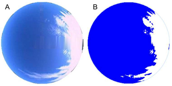
Figure 3.
A representation of the sky over CIESOL center. (A) image, represents the original sky cam image; (B) image, the processed sky camera image.
In order to study cloud movement, the following steps are taken [18]:
- The picture taken with the sky camera is divided into the different sectors given in Figure 4, since the movement of the clouds will depend on the sector covered by the sky camera.
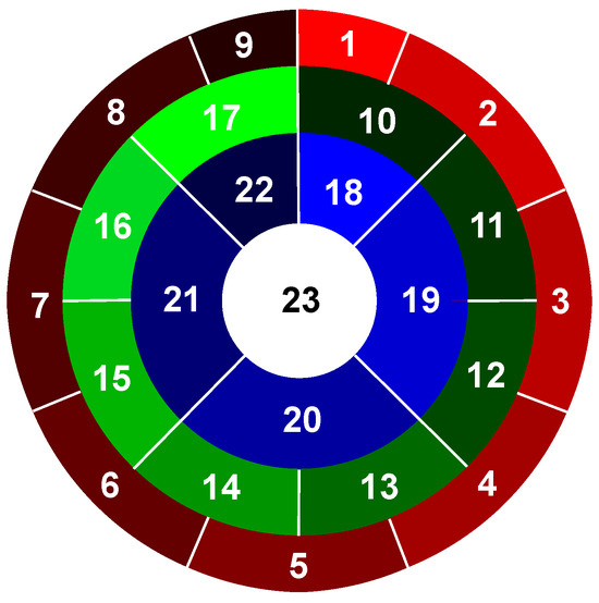 Figure 4. Sky camera image division into 23 sectors.
 - The cloud motion vector (CMV) is calculated for each sector by applying the maximum cross-correlation method.
- Different quality tests are applied to ensure the correct determination of the cloud motion.
The CMV is applied to the last image received and re-applied to the result obtained. This process is repeated up to 30 times (prediction for 30 min ahead), obtaining the movement of the pixels from the minute in which the image was taken to the 30th minute in the future. Therefore, each application of the CMV is 1 min of forecasting. Finally, the prediction of cloud presence consists of checking if the new position of the clouds masks the future sun’s path.
According to the sequence of sky cam images used, one-minute forecasting is considered an appropriate interval to study the cloud movement. Having a lower interval (i.e., a lower time between scenes and lower temporal horizons in the forecasting) will result in an important computational time. On the other hand, increasing the interval to several minutes leads to a loss of information because of the rapid movement of clouds.
4. Post-Processing with Binary Probabilistic Models
In the literature, three main categories of statistical models are proposed to generate probabilistic forecasts of binary events [31]. The first family of models, called parametric, assumes that the probability of the event follows a known distribution law, such as Gaussian or logistic. Conversely, the second type of models, called non-parametric, is not based on underlying distributions. Predictions are learned from a sample of data and, obviously, machine learning techniques dominate this second family of models. The last category, called semi-parametric, is a mix of the two previous ones. In this work, we proposed to test two parametric models and one non-parametric model to post-process the deterministic forecasts.
4.1. Parametric Approach
The first approach proposed here is based on the very well-known statistical models logit and probit used for decision-making problems involving binary or categorical choices in various domains such as economy [16] or meteorology [32]. These two parametric models belong to the generalized linear models (GLM) [33]. Their aim is to model the probabilities of a random response variable Y as a function of some explanatory variables. The model combines two functions. First, a function, called index function or systematic component, associates independent explanatory variables within a linear or non-linear model. Second, a link function links the systematic component with the random response variable.
For the logit and probit models, the index function Z is a linear combination of independent explanatory variables (, …, ) and corresponding regression coefficients (, …, ), written as follows:
Used alone, this linear function is not able to provide suitable probability levels. Indeed, linear functions are not bounded in the range . To overcome this issue, link functions have been proposed to transform the result of the index function Z into probabilities ranging between 0 (i.e., cloud) and 1 (i.e., no cloud). In our case, only the link function differentiates the logit and probit models. For the logit model, the link function is the following logistic function (also called sigmoid function):
For the probit model, the link function is the cumulative standard normal distribution function given below:
The input variables of these models can be either continuous, binary, or categorical. This feature is very important in our case because the explanatory variables available to generate probabilistic forecasts of the cloud presence are binary (i.e., the deterministic forecasts) and continuous (i.e., measured irradiance, solar zenith angle, hour of the day, etc.). The main difference between these two parametric models is the shape of the link function. The logistic function produces heavier tails than the standard normal distribution function. To implement the logit and probit models, we used the “glm” function of the package “stats” that is part of R [34], which is based on the maximum likelihood approach to estimate the coefficients.
4.2. Non-Parametric Approach
As most real-life phenomena do not follow a known distribution law, non-parametric models have been developed. Non-parametric binary choice models have been initially developed for economic applications [35]. A set of non-parametric regressions, designed for continuous variables and also suitable for binary events probability, are available in the literature [36,37]. The main challenge for these regression models is to combine continuous, categorical, and binary data as input [38], like in our work.
Decision trees (DT) and, by extension, random forests (RF), which belong to the supervised machine learning methods, are appealing non-parametric models to predict discrete choice. Indeed, they can predict either a numerical value (regression tree), a class, or a discrete choice (classification tree). They can use either continuous, categorical, or binary variables as input. They require less computational effort than classical non-parametric regression methods. Indeed, the computation time of regression methods increases exponentially with the number of variables which is not the case for DT and RF.
The characteristics of the RF used in this work are introduced by [39]. The readers may refer to [40] for a general presentation. A classification tree is a decision tool that estimates the most likely class of a categorical or a binary variable to predict when the input variables are known. Decision trees are simple models that partition the features (or inputs) space into subsets [40]. An iterative algorithm is used to split the input space. At each step or node, the data are divided into two subsets, applying an “If, Then” rule to one of the input variables. At each step, the selected input is chosen to provide the best possible separation of the classes to predict. The aim is to generate the optimal sequences of rules to predict the different possible classes [39].
An RF is a set of trees that are built on bootstrapped training subsets. Several decision trees are therefore trained. When RF are used as classifiers, the probabilities of the predicted classes are averaged from the answers of the individual trees, as illustrated in Figure 5. In the RF, the strengths (and weaknesses) of each tree are aggregated. A cross-validation was done on the number of trees and a good trade-off was obtained for 500 trees. In this work, we used the RF classifier algorithm implemented in the R package “randomForest” based on [41].
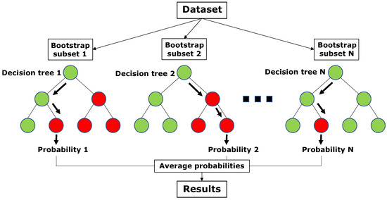
Figure 5.
Simplified illustration of a random forest classifier used to predict class probability.
4.3. Implementation
As previously introduced and presented in Figure 1, the forecasting process has two main steps: generation of deterministic forecast from the sky imager and post-processing with the probabilistic models. The first step is briefly detailed in Section 3. Here, we will focus on the implementation of the probabilistic models. The simplest approach is to use only the discrete cloud forecast as input of the probabilistic model. However, numerous works show that the addition of inputs, such as past observations or solar path variables, can significantly improve the quality of solar forecasts generated by time series models [42] or post-processing methods [43,44]. Thus, to improve the performance of the post-processing step, we tested the addition of easy-to-compute variables as input to the three tested probabilistic models. The tested additional variables are: solar zenith angle, current and past global horizontal irradiances, beam normal irradiances and clear sky indices, and mean and variability over past observed clear sky indices. The best combination of inputs, based on the BS, is as follows:
- The deterministic forecast of cloud presence ;
- The current clear sky index ;
- The mean over the five past clear sky indices .
Finally, we created one post-processing model by forecast horizon. Considering a time resolution of 1 min and horizons up to 30 min, we trained 30 different models for each of the three probabilistic methods presented above.
5. Case Study and Data
In this study, images from a sky camera with a rotational shadow band (TSI-880 model) have been used to provide a hemispheric vision of sky (fish-eye vision). Additionally, the measurements of diffuse and global irradiance from two CMP Kipp & Zonen pyranometers and direct irradiance from a CH1 Kipp & Zonen pyrheliometer were used, and all the instruments were installed on a two-axis solar tracker. The testing facility is located at the Center of Research of Solar Energy (CIESOL) at the University of Almería in a region in southern Spain. The facility has a Mediterranean climate with a large presence of maritime aerosols and is located at 36.8 N latitude and 2.4 W longitude at sea level. Data are collected every minute, as this was proposed to be a suitable frequency [3]. Appropriate maintenance was performed on the sensors and sky camera. The sensors are cleaned with ethyl alcohol every day. The sky camera mirror is cleaned using a soft rag with distilled water three times a week. Figure 6 shows the sky cam installed on the roof of CIESOL.
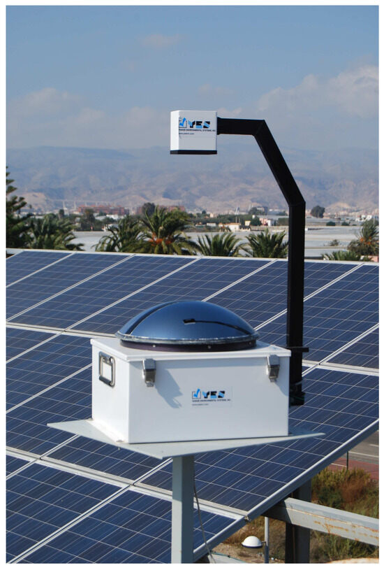
Figure 6.
TSI-880 installed in CIESOL.
Images were taken with 352 × 288 color pixel resolution, which corresponds to 24 bits in JPEG format. They have three different channels that represent the red, green, and blue levels. Each pixel of the image is represented by 8 bits, with values between 0 and 255.
For the cloud now casting, data from 2010 and 2011 were used, for moments where the solar altitude degree was higher than 5. For 2010, a total of 137,794 moments were analyzed for each interval of prediction (1 to 30 min) independently, whereas for 2011, 134,993 predictions were processed, also for each forecast interval. The year 2010 was used to train the post-processing models and the year 2011 was used to test them.
It should be noted that the number of observation/forecast pairs and the ratio of observed cloudless skies in the test set (2011) are not identical for the different forecast horizons. Indeed, the ASI fails to predict the presence of clouds for long horizons when the cloud speed is high and/or when the cloud base height is low. Specifically, under these conditions, predicted cloud locations have a high probability of leaving the ASI’s field of view before a horizon of 30 min. As a consequence, the total number of observation/forecast pairs decreases while the ratio of observed cloudless skies in the test set slightly increases with the forecast horizon as presented in Figure 7. As the clear skies are easier to forecast, this pattern will impact the assessment of the model’s accuracy.
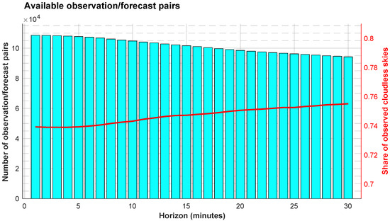
Figure 7.
Number of observation/forecast pairs (blue bars) and ratio of observed cloudless skies (red line) in the test set (2011) for forecast horizons ranging from 1 to 30 min.
6. Results and Discussion
The post-processing of the deterministic forecasts gives a probability level of the possible future cloud presence. But, it can also be seen as a calibration of the deterministic forecasts based on the training set statistics. Furthermore, it is common to transform the probability level resulting from the discrete choice models in new binary and deterministic forecasts. Indeed, considering a perfectly calibrated probabilistic forecast (i.e., for a forecast probability of x%, we observed x% of yes event), a threshold set at a probability of 50% to make a decision (event or no event) maximizes the accuracy of the resulting deterministic forecast. This assumption is discussed in Appendix B. Therefore, to convert a probabilistic forecast into a deterministic one, we assume that a probability above 0.5 (>50%) corresponds to a “yes” event, i.e., in our case a clear sky, whereas a probability below 0.5 (<50%) is a “no” event corresponding to the presence of clouds. To assess the ability of the selected discrete choice models to improve the deterministic forecast, this transformation was applied to the probabilistic forecasts. Thus, the evaluation of the generated forecasts will be performed in two steps. First, we will evaluate the improvement of the quality of the deterministic forecasts before and after the post-processing step. Second, we will assess the quality of the probabilistic forecasts and the improvement compared to the corresponding deterministic forecasts. Table A1 provided in Appendix A, gives the detailed numeric results used to plot the graphs evaluating the quality of the forecasts.
6.1. Deterministic Forecasts Quality
Figure 8 shows the evaluation of the quality of the deterministic forecasts before and after the post-processing with the three discrete choice models tested in this work. Surprisingly, with longer horizons, the accuracy of the initial forecasts done with the sky imager increases (solid black line). This observation results from the share of clear and cloudy skies available in the test sets presented previously in Section 5 and Figure 7. Indeed, for longer horizons, the share of clear skies, which are easier to forecast when there is no cloud in the field of view of the ASI, is more important. We could have homogenized the test sets of the different horizons to cancel this effect. However, removing conditions with fast-moving clouds from the shorter horizons would have biased the analysis of the improvement brought by the probabilistic approach which is more interesting when forecasting becomes more uncertain. Even if this effect does not influence significantly the results of this work, the reader must keep in mind that for the longest horizons, the test sets lead to a higher share of situations that are easier to forecast [3,45].
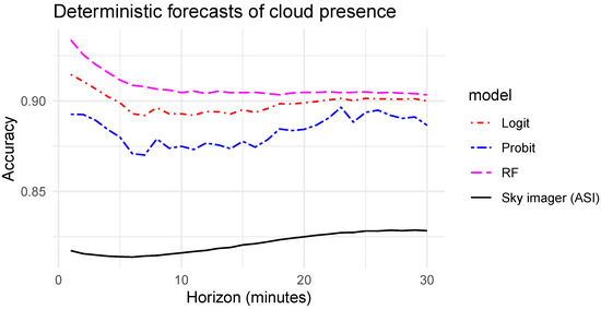
Figure 8.
Accuracy (or fraction correct) of the deterministic forecasts before (sky imager (ASI)) and after the post-processing by the 3 discrete choice models (Logit, Probit, and RF).
As expected, the post-processing with the discrete choice models improves significantly the accuracy of the forecasting system. For horizons from 1 to 15 min, the accuracy resulting from the three models decreases. Above a 15 min horizon, as for the original ASI forecasts, the accuracy increases slightly. Among the three tested models, the RF model, which is a non-parametric method, shows the best improvement with an accuracy of 93.4% and 90.3% for horizons of 1 min and 30 min respectively. Compared to the initial ASI forecasts, this improvement corresponds to a gain of 11.6 percentage points for the shortest horizon (i.e., 1 min) and 7.5 percentage points for the longest one (i.e., 30 min). Regarding the two parametric techniques, the logit model, which has an accuracy close to the RF, clearly outperforms the probit model. However, both of them show a significant improvement over the ASI original forecasts. Given the simplicity and the low computational efforts of the logit model, the former offers a very good trade-off for the study case selected in this work.
6.2. Probabilistic Forecasts Quality
As previously discussed in Section 2, the reliability of the probabilistic forecast is the first attribute to verify. Figure 9 gives the reliability diagrams of the three discrete choice models and of the climatology model for all the horizons of forecast (i.e., overall reliability). The climatology is a very simple model used as a reference, which forecasts the average probability of the event whatever the weather conditions and the horizon. Here, the average probability of having a clear sky computed from the test set is 74.8%. The reliability diagram is a visual tool that gives a qualitative assessment of the reliability. It plots the correspondence between the forecast probability (x axis) and the observed frequency of the event (y axis). A perfectly reliable model should result in a reliability curve that sticks to the diagonal. Here, none of the three tested models presents perfect reliability. Conversely to the RF models, the probit and logit models never generate forecast probabilities of 0 and 1. As a consequence, their reliability curves do not reach the lower and upper limits of the diagram. The important deviations from the diagonal of the probit and logit models indicate a peak of underconfidence for a forecast probability of 0.5 and overconfidence for forecast probabilities ranging between 0.75 and 0.9. In other words, when these two models issue a forecast probability of 0.5 (i.e., 50% probability of a clear sky), the actual observed frequency is higher than 0.75. The RF model shows a better overall reliability than the two parametric models with a high reliability when it forecasts a clear sky with forecast probabilities above 0.5.
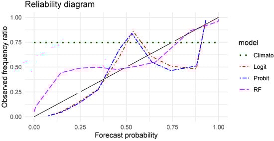
Figure 9.
Reliability diagrams of the 3 discrete choice models and of the climatology.
The second interesting attribute to verify is the resolution, which corresponds to the ability of a forecasting system to issue case dependent forecasts. Figure 10 gives the ROC curves of the four probabilistic models evaluated in this work. A perfect resolution will lead to a curve that sticks to the y axis, i.e., a false alarm rate equal to zero, and then follows the line with a hit rate equal to 1. Thus, the higher the area under the ROC curve, the better the resolution. The climatology, which always gives the same forecast, has no resolution and follows the diagonal. The probit and the logit models have exactly the same resolution. The quality of their forecast depends only on their reliability. Finally, the RF model shows a better resolution than the other methods. As the RF model also has better reliability, its overall quality evaluated with a proper score should be the best.
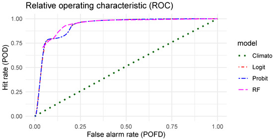
Figure 10.
ROC curves of the 3 discrete choice models and of the climatology.
In addition to the reliability and resolution assessment, the BS and the corresponding SS provide quantitative information on the quality of the forecast. The BS is negatively oriented and a lower value indicates better quality. Figure 11 shows the BS of the original ASI forecasts, of the climatology model, based on the training set, and of the three discrete choice models. For the original ASI forecasts (solid black line), which are deterministic, the BS is derived from the accuracy as detailed in Section 2. First, we can observe that the quality of the climatology increases slightly with the horizon. Again, this trend results from the increased share of clear skies for the longer horizons in the test set. However, the SS given in Table A1, which gives the relative improvement over the climatology, shows that the relative efficiency of the three tested models decreases while the horizon of forecast increases. Second, the BS of the probit and logit models is almost the same regardless of the horizon. This result, which differs from that obtained with their deterministic counterparts, highlights that the information included in a probabilistic forecast cannot be translated into a deterministic forecast. Finally, the RF model clearly outperforms the two parametric models. The good performance of this non-parametric model comes from several advantages. Indeed, RF is able to map non-linear relationships between inputs and outputs. It is designed to handle different types of variables, which can be binary, categorical, or continuous. Finally, unlike probit and logit models, RF issues probability forecasts of 0 and 1 with high reliability.
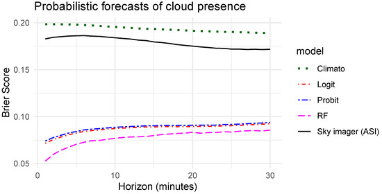
Figure 11.
BS scores of the original ASI forecasts, of the climatology model used as a reference, and of the probabilistic forecasts resulting from post-processing with the 3 discrete-choice models.
In this work, we propose an alternative method to evaluate the probability associated with a solar forecast. Until now, the developed forecasting models are calibrated on arbitrarily fixed probability levels. The resulting outputs are the associated quantiles of the future available solar energy. In this work, the calibration works in the opposite way. We defined a solar irradiance level (here 400 Wm) and our models give the probability of overtaking this threshold. This approach, based on a single threshold, is well suited to CSP plant operation, which requires anticipating the starting and stopping conditions. However, one can imagine applying the same approach to evaluate the probabilities of exceeding a set of arbitrarily chosen solar energy thresholds. As no other work proposes a similar binary solar forecast, it is currently impossible to compare our results with previously developed models. With the aim of making our results suitable for future comparison, we proposed a comprehensive testing procedure. Indeed, the selected tools and metrics, which come from other domains such as meteorology and economy, allow evaluation of the main attributes of the forecast quality.
7. Conclusions
This work is the first attempt, in the field of solar energy, to propose a methodology to generate very short-term probabilistic forecasts as a binary event. The objective is to anticipate the moment when the direct normal irradiance is higher than a defined threshold, suitable to the operation of concentrated solar power plants. The proposed approach combines binary forecast based on a sky imager with discrete choice models commonly used in various decision-making problems to generate a probability forecast of cloud presence. Two parametric (probit and logit) models and one non-parametric (RF) discrete choice model have been tested in this work. The RF clearly outperforms the widely used probit and logit models. Beyond a better quality assessed with the reliability diagram, the ROC, and the BS, the RF provides better features, like the ability to forecast probability levels of 0 or 1 with high reliability.
As this work is the first one on the topic, no comparison with other models or approaches is possible and it is difficult to evaluate the actual performance of the proposed method. However, the generated forecasts show a good quality. Indeed, the accuracy of the deterministic forecasts derived from the probability level is above 90% with an improvement ranging from 7.5 to 11.6 percentage points compared to the original ASI forecasts. Regarding the probability forecasts obtained with the three tested models, their BS is below 0.1, regardless of the horizon of the forecast.
Author Contributions
Conceptualization, M.D. and J.A.-M.; methodology, M.D. and J.A.-M.; validation, M.D. and J.L.G.L.S.; formal analysis, M.D.; investigation, M.D.; resources, M.D. and J.A.-M.; data curation, M.D. and J.A.-M.; writing—original draft preparation, M.D. and J.A.-M.; writing—review and editing, J.L.G.L.S. and P.L.; visualization, M.D.; supervision, M.D.; project administration, M.D.; funding acquisition, M.D. and J.A.-M. All authors have read and agreed to the published version of the manuscript.
Funding
This research was funded by the Ministerio de Ciencia e Innovación reference PID2020-118239RJ-I00 and co-financed by the European Regional Development Fund for the project MAPVSpain. This research also received support from the TwInSolar project funded by the European Union’s Horizon Europe research and innovation program grant number 101076447.
Data Availability Statement
The data presented in this study are available on request from the corresponding author. The data are not publicly available because they were obtained as part of a project with a private company and the regional government.
Conflicts of Interest
The authors declare no conflict of interest.
Abbreviations
The following abbreviations are used in this manuscript:
| ASI | All Sky Imager |
| BS | Brier Score |
| CIESOL | Center of Research of Solar Energ |
| CMV | Cloud Motion Vector |
| CSP | Concentrated Solar Plant |
| DNI | Direct Normal Irradiance |
| DT | Decision Trees |
| FAR | False Alarm Ratio |
| GLM | Generalized Linear Models |
| MSG | MeteoSat Second Generation |
| NWP | Numerical Weather Prediction |
| POD | Probability Of Detection |
| POFD | Probability Of False Detection |
| PV | Photovolatic |
| RF | Random Forest |
| RMSE | Root Mean Square Error |
| ROC | Relative Operating Characteristic |
| SR | Success Rate |
| SS | Skill Score |
Appendix A. Numerical Results of Forecast Evaluation

Table A1.
Numerical results of the evaluation of deterministic and probabilistic forecasts for the different horizons.
Table A1.
Numerical results of the evaluation of deterministic and probabilistic forecasts for the different horizons.
| Horizon | Accuracy | BS | SS | ||||||||
|---|---|---|---|---|---|---|---|---|---|---|---|
| (Minutes) | ASI | Probit | Logit | RF | Climato | Probit | Logit | RF | Probit | Logit | RF |
| 1 | 0.817 | 0.893 | 0.915 | 0.934 | 0.198 | 0.074 | 0.072 | 0.053 | 0.626 | 0.636 | 0.732 |
| 2 | 0.815 | 0.892 | 0.911 | 0.925 | 0.198 | 0.078 | 0.075 | 0.059 | 0.606 | 0.621 | 0.702 |
| 3 | 0.814 | 0.889 | 0.907 | 0.920 | 0.198 | 0.080 | 0.078 | 0.064 | 0.596 | 0.606 | 0.677 |
| 4 | 0.814 | 0.884 | 0.902 | 0.916 | 0.198 | 0.082 | 0.081 | 0.067 | 0.586 | 0.591 | 0.662 |
| 5 | 0.813 | 0.880 | 0.899 | 0.911 | 0.198 | 0.084 | 0.082 | 0.071 | 0.576 | 0.586 | 0.641 |
| 6 | 0.813 | 0.871 | 0.893 | 0.909 | 0.198 | 0.086 | 0.084 | 0.073 | 0.566 | 0.576 | 0.631 |
| 7 | 0.814 | 0.870 | 0.892 | 0.908 | 0.197 | 0.087 | 0.085 | 0.074 | 0.558 | 0.569 | 0.624 |
| 8 | 0.814 | 0.879 | 0.896 | 0.906 | 0.197 | 0.087 | 0.086 | 0.075 | 0.558 | 0.563 | 0.619 |
| 9 | 0.815 | 0.874 | 0.893 | 0.906 | 0.196 | 0.088 | 0.087 | 0.076 | 0.551 | 0.556 | 0.612 |
| 10 | 0.816 | 0.875 | 0.893 | 0.905 | 0.196 | 0.089 | 0.087 | 0.077 | 0.546 | 0.556 | 0.607 |
| 11 | 0.816 | 0.873 | 0.892 | 0.905 | 0.195 | 0.089 | 0.088 | 0.078 | 0.544 | 0.549 | 0.600 |
| 12 | 0.817 | 0.877 | 0.894 | 0.904 | 0.194 | 0.089 | 0.088 | 0.078 | 0.541 | 0.546 | 0.598 |
| 13 | 0.818 | 0.876 | 0.894 | 0.905 | 0.194 | 0.090 | 0.088 | 0.078 | 0.536 | 0.546 | 0.598 |
| 14 | 0.819 | 0.874 | 0.893 | 0.905 | 0.194 | 0.090 | 0.089 | 0.079 | 0.536 | 0.541 | 0.593 |
| 15 | 0.820 | 0.878 | 0.895 | 0.905 | 0.193 | 0.090 | 0.089 | 0.080 | 0.534 | 0.539 | 0.585 |
| 16 | 0.821 | 0.874 | 0.894 | 0.905 | 0.193 | 0.091 | 0.089 | 0.081 | 0.529 | 0.539 | 0.580 |
| 17 | 0.822 | 0.878 | 0.896 | 0.904 | 0.193 | 0.091 | 0.089 | 0.081 | 0.528 | 0.539 | 0.580 |
| 18 | 0.823 | 0.884 | 0.898 | 0.903 | 0.192 | 0.091 | 0.089 | 0.082 | 0.526 | 0.536 | 0.573 |
| 19 | 0.824 | 0.884 | 0.898 | 0.904 | 0.192 | 0.091 | 0.089 | 0.082 | 0.526 | 0.536 | 0.573 |
| 20 | 0.824 | 0.884 | 0.899 | 0.905 | 0.191 | 0.091 | 0.089 | 0.083 | 0.524 | 0.534 | 0.565 |
| 21 | 0.825 | 0.887 | 0.900 | 0.905 | 0.191 | 0.091 | 0.090 | 0.082 | 0.524 | 0.529 | 0.571 |
| 22 | 0.826 | 0.891 | 0.901 | 0.905 | 0.191 | 0.091 | 0.090 | 0.083 | 0.524 | 0.529 | 0.565 |
| 23 | 0.827 | 0.896 | 0.901 | 0.905 | 0.191 | 0.091 | 0.090 | 0.083 | 0.524 | 0.529 | 0.565 |
| 24 | 0.827 | 0.888 | 0.900 | 0.905 | 0.190 | 0.092 | 0.090 | 0.084 | 0.516 | 0.526 | 0.558 |
| 25 | 0.828 | 0.894 | 0.901 | 0.905 | 0.190 | 0.092 | 0.090 | 0.084 | 0.516 | 0.526 | 0.558 |
| 26 | 0.828 | 0.895 | 0.901 | 0.904 | 0.190 | 0.092 | 0.091 | 0.084 | 0.516 | 0.521 | 0.558 |
| 27 | 0.828 | 0.892 | 0.901 | 0.905 | 0.190 | 0.092 | 0.091 | 0.085 | 0.516 | 0.521 | 0.553 |
| 28 | 0.828 | 0.890 | 0.901 | 0.904 | 0.189 | 0.093 | 0.092 | 0.085 | 0.508 | 0.513 | 0.550 |
| 29 | 0.828 | 0.891 | 0.901 | 0.904 | 0.189 | 0.093 | 0.092 | 0.085 | 0.508 | 0.513 | 0.550 |
| 30 | 0.828 | 0.887 | 0.900 | 0.903 | 0.189 | 0.094 | 0.092 | 0.086 | 0.503 | 0.513 | 0.545 |
| Overall | 0.821 | 0.883 | 0.899 | 0.908 | 0.198 | 0.088 | 0.087 | 0.077 | 0.556 | 0.561 | 0.611 |
Appendix B. Discussion on the Threshold Used to Convert Probability Forecasts to Deterministic Forecasts
To define the probability threshold used to convert the probabilistic forecasts into deterministic ones, we assume in this work a perfect calibration of the discrete choice models. This assumption leads to taking a threshold of 50% to make a decision between a clear sky and a cloudy sky. However, the three discrete choice models tested do not systematically generate perfectly calibrated forecasts as shown in Figure 9. One can imagine defining a probability threshold that actually maximizes the accuracy of the derived deterministic forecasts. Figure A1 gives the evolution of the accuracy of the deterministic forecasts derived from the three discrete choice models for a probability threshold ranging from 0% to 100%. To plot this figure, we aggregated forecasts obtained with the training set from all the considered horizons, from 1 to 30 min. The maximum accuracies appear with probabilities of 47% and 48% for the probit and logit models, respectively. At these maximums, the resulting accuracies are extremely close to the ones observed for a threshold taken at 50% (i.e., a deviation of 0.0027 for the probit model and 0.0013 for the logit model). Regarding the RF model, the accuracy remains almost constant for probabilities ranging from 25% to 75% with a variation of accuracy that does not exceed 0.0022 in this interval. These results confirm the hypothesis of well-calibrated forecasts on the training set.
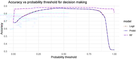
Figure A1.
Evolution of the accuracy for a probability threshold ranging from 0% to 100%. This threshold is used to convert the probabilistic forecasts into deterministic forecasts for the training set (year 2010).
To better understand the very small deviations in accuracy observed around a threshold of 50%, Figure A2 shows the distributions of the probability forecasts generated by the three discrete choice models. Almost all the forecast probabilities are below 25% and above 75%. As a consequence, choosing a threshold around the actual maximum, which is close to a 50% probability will not affect significantly the value of the resulting accuracy. It is worth noting that these observations are based on the training set. Indeed, building a model or in our case selecting the most suitable threshold to derive the deterministic forecasts must rely only on the training data. To conclude, these results support the initial assumption of a perfectly calibrated probabilistic forecast used to select a threshold of 50%.
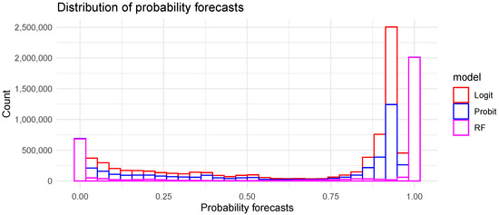
Figure A2.
Distribution of the probability forecast of three discrete choice models for the training set (year 2010).
References
- Diagne, M.; David, M.; Lauret, P.; Boland, J.; Schmutz, N. Review of solar irradiance forecasting methods and a proposition for small-scale insular grids. Renew. Sustain. Energy Rev. 2013, 27, 65–76. [Google Scholar] [CrossRef]
- Antonanzas, J.; Osorio, N.; Escobar, R.; Urraca, R.; de Pison, F.M.; Antonanzas-Torres, F. Review of photovoltaic power forecasting. Sol. Energy 2016, 136, 78–111. [Google Scholar] [CrossRef]
- Lorenz, E.; Ruiz-Arias, J.A.; Martin, L.; Wilbert, S.; Köhler, C.; Fritz, R.; Betti, A.; Lauret, P.; David, M.; Huang, J.; et al. Forecasting Solar Radiation and Photovoltaic Power. In Best Practices Handbook for the Collection and Use of Solar Resource Data for Solar Energy Applications, 3rd ed.; National Renewable Energy Laboratory: Golden, CO, USA, 2021. [Google Scholar]
- Arnaoutakis, G.E.; Katsaprakakis, D.A. Concentrating Solar Power Advances in Geometric Optics, Materials and System Integration. Energies 2021, 14, 6229. [Google Scholar] [CrossRef]
- Marquez, R.; Coimbra, C.F. Intra-hour DNI forecasting based on cloud tracking image analysis. Sol. Energy 2013, 91, 327–336. [Google Scholar] [CrossRef]
- Nouri, B.; Noureldin, K.; Schlichting, T.; Wilbert, S.; Hirsch, T.; Schroedter-Homscheidt, M.; Kuhn, P.; Kazantzidis, A.; Zarzalejo, L.; Blanc, P.; et al. Optimization of parabolic trough power plant operations in variable irradiance conditions using all sky imagers. Sol. Energy 2020, 198, 434–453. [Google Scholar] [CrossRef]
- Ajith, M.; Martínez-Ramón, M. Deep learning algorithms for very short term solar irradiance forecasting: A survey. Renew. Sustain. Energy Rev. 2023, 182, 113362. [Google Scholar] [CrossRef]
- Alonso-Montesinos, J.; Batlles, F.; Portillo, C. Solar irradiance forecasting at one-minute intervals for different sky conditions using sky camera images. Energy Convers. Manag. 2015, 105, 1166–1177. [Google Scholar] [CrossRef]
- Logothetis, S.A.; Salamalikis, V.; Wilbert, S.; Remund, J.; Zarzalejo, L.F.; Xie, Y.; Nouri, B.; Ntavelis, E.; Nou, J.; Hendrikx, N.; et al. Benchmarking of solar irradiance nowcast performance derived from all-sky imagers. Renew. Energy 2022, 199, 246–261. [Google Scholar] [CrossRef]
- Alonso-Montesinos, J.; Monterreal, R.; Fernandez-Reche, J.; Ballestrín, J.; López, G.; Polo, J.; Barbero, F.J.; Marzo, A.; Portillo, C.; Batlles, F.J. Nowcasting System Based on Sky Camera Images to Predict the Solar Flux on the Receiver of a Concentrated Solar Plant. Remote Sens. 2022, 14, 1602. [Google Scholar] [CrossRef]
- Paletta, Q.; Arbod, G.; Lasenby, J. Omnivision forecasting: Combining satellite and sky images for improved deterministic and probabilistic intra-hour solar energy predictions. Appl. Energy 2023, 336, 120818. [Google Scholar] [CrossRef]
- Nouri, B.; Wilbert, S.; Blum, N.; Fabel, Y.; Lorenz, E.; Hammer, A.; Schmidt, T.; Zarzalejo, L.F.; Pitz-Paal, R. Probabilistic solar nowcasting based on all-sky imagers. Sol. Energy 2023, 253, 285–307. [Google Scholar] [CrossRef]
- Hong, T.; Pinson, P.; Fan, S.; Zareipour, H.; Troccoli, A.; Hyndman, R.J. Probabilistic energy forecasting: Global Energy Forecasting Competition 2014 and beyond. Int. J. Forecast. 2016, 32, 896–913. [Google Scholar] [CrossRef]
- van der Meer, D.; Widén, J.; Munkhammar, J. Review on probabilistic forecasting of photovoltaic power production and electricity consumption. Renew. Sustain. Energy Rev. 2018, 81, 1484–1512. [Google Scholar] [CrossRef]
- Alonso-Montesinos, J.; Polo, J.; Ballestrín, J.; Batlles, F.; Portillo, C. Impact of DNI forecasting on CSP tower plant power production. Renew. Energy 2019, 138, 368–377. [Google Scholar] [CrossRef]
- McFadden, D.L. Econometric models of probabilistic choice. In Structural Analysis of Discrete Data with Econometric Applications; Manski, C.F., McFadden, D.L., Eds.; MIT Press: Cambridge, MA, USA, 1981; pp. 198–272. [Google Scholar]
- Wilks, D.S. Statistical Methods in the Atmospheric Sciences, 2nd ed.; Number 91 in International Geophysics Series; Elsevier: Amsterdam, The Netherlands, 2009. [Google Scholar]
- Alonso, J.; Batlles, F. Short and medium-term cloudiness forecasting using remote sensing techniques and sky camera imagery. Energy 2014, 73, 890–897. [Google Scholar] [CrossRef]
- Kraas, B.; Schroedter-Homscheidt, M.; Madlener, R. Economic merits of a state-of-the-art concentrating solar power forecasting system for participation in the Spanish electricity market. Sol. Energy 2013, 93, 244–255. [Google Scholar] [CrossRef]
- Escrig, H.; Batlles, F.J.; Alonso, J.; Baena, F.M.; Bosch, J.L.; Salbidegoitia, I.B.; Burgaleta, J.I. Cloud detection, classification and motion estimation using geostationary satellite imagery for cloud cover forecast. Energy 2013, 55, 853–859. [Google Scholar] [CrossRef]
- Yang, D.; Alessandrini, S.; Antonanzas, J.; Antonanzas-Torres, F.; Badescu, V.; Beyer, H.G.; Blaga, R.; Boland, J.; Bright, J.M.; Coimbra, C.F.; et al. Verification of deterministic solar forecasts. Sol. Energy 2020, 210, 20–37. [Google Scholar] [CrossRef]
- Lauret, P.; David, M.; Pinson, P. Verification of solar irradiance probabilistic forecasts. Sol. Energy 2019, 194, 254–271. [Google Scholar] [CrossRef]
- Gneiting, T.; Lerch, S.; Schulz, B. Probabilistic solar forecasting: Benchmarks, post-processing, verification. Sol. Energy 2023, 252, 72–80. [Google Scholar] [CrossRef]
- Murphy, A.H. What Is a Good Forecast? An Essay on the Nature of Goodness in Weather Forecasting. Weather Forecast. 1993, 8, 281–293. [Google Scholar] [CrossRef]
- Brooks, H.; Brown, B.; Brown, B.; Ferro, C.; Jolliffe, J.; Koh, T.Y.; Roebber, P.; Stephenson, D. Joint Working Group on Forecast Verification Research. 2015. Available online: https://cawcr.gov.au/projects/verification/ (accessed on 8 October 2023).
- Hogan, R.J.; Mason, I.B. Deterministic Forecasts of Binary Events. In Forecast Verification; John Wiley & Sons, Ltd.: Hoboken, NJ, USA, 2011. [Google Scholar] [CrossRef]
- Pinson, P.; Nielsen, H.A.; Møller, J.K.; Madsen, H.; Kariniotakis, G.N. Non-parametric probabilistic forecasts of wind power: Required properties and evaluation. Wind Energy 2007, 10, 497–516. [Google Scholar] [CrossRef]
- Hamill, T.M. Reliability Diagrams for Multicategory Probabilistic Forecasts. Weather Forecast. 1997, 12, 736–741. [Google Scholar] [CrossRef]
- Jolliffe, I.; Stephenson, D. Forecast Verification: A Practitioner’s Guide in Atmospheric Science; Wiley: Hoboken, NJ, USA, 2012. [Google Scholar]
- Alonso, J.; Batlles, F.J.; Ternero, A.; López, G. Sky camera imagery processing based on a sky classification using radiometric data. Energy 2014, 68, 599–608. [Google Scholar] [CrossRef]
- Lahiri, K.; Yang, L. Chapter 19—Forecasting Binary Outcomes. In Handbook of Economic Forecasting; Elliott, G., Timmermann, A., Eds.; Elsevier: Amsterdam, The Netherlands, 2013; Volume 2, pp. 1025–1106. [Google Scholar] [CrossRef]
- Sánchez, J.; Marcos, J.; de la Fuente, M.; Castro, A. A logistic regression model applied to short term forecast of hail risk. Phys. Chem. Earth 1998, 23, 645–648. [Google Scholar] [CrossRef]
- McCullagh, P.; Nelder, J.A. Generalized Linear Models; Springer: Boston, MA, USA, 1989. [Google Scholar] [CrossRef]
- R Core Team. R: A Language and Environment for Statistical Computing; R Foundation for Statistical Computing: Vienna, Austria, 2022; ISBN 3-900051-07-0. [Google Scholar]
- Frölich, M. Non-parametric regression for binary dependent variables. Econom. J. 2006, 9, 511–540. [Google Scholar] [CrossRef]
- Li, Q.; Racine, J.S. Nonparametric Econometrics: Theory and Practice; Princeton University Press: Princeton, NJ, USA, 2007. [Google Scholar]
- Newey, W.K. Nonparametric Continuous/Discrete Choice Models. Int. Econ. Rev. 2007, 48, 1429–1439. [Google Scholar] [CrossRef]
- Li, Q.; Racine, J.S. Nonparametric Estimation of Conditional CDF and Quantile Functions With Mixed Categorical and Continuous Data. J. Bus. Econ. Stat. 2008, 26, 423–434. [Google Scholar] [CrossRef]
- Breiman, L.; Friedman, J.H.; Olshen, R.A.; Stone, C.J. Classification and Regression Trees; Routledge: Oxfordshire, UK, 2017. [Google Scholar]
- Hastie, T.; Tibshirani, R.; Friedman, J. The Elements of Statistical Learning; Springer Series in Statistics; Springer: New York, NY, USA, 2009. [Google Scholar]
- Breiman, L. Random Forests. Mach. Learn. 2001, 45, 5–32. [Google Scholar] [CrossRef]
- Grantham, A.; Gel, Y.R.; Boland, J. Nonparametric short-term probabilistic forecasting for solar radiation. Sol. Energy 2016, 133, 465–475. [Google Scholar] [CrossRef]
- Lorenz, E.; Hurka, J.; Heinemann, D.; Beyer, H.G. Irradiance Forecasting for the Power Prediction of Grid-Connected Photovoltaic Systems. IEEE J. Sel. Top. Appl. Earth Obs. Remote Sens. 2009, 2, 2–10. [Google Scholar] [CrossRef]
- Huang, J.; Perry, M. A semi-empirical approach using gradient boosting and k-nearest neighbors regression for GEFCom2014 probabilistic solar power forecasting. Int. J. Forecast. 2016, 32, 1081–1086. [Google Scholar] [CrossRef]
- Quesada-Ruiz, S.; Chu, Y.; Tovar-Pescador, J.; Pedro, H.; Coimbra, C. Cloud-tracking methodology for intra-hour DNI forecasting. Sol. Energy 2014, 102, 267–275. [Google Scholar] [CrossRef]
Disclaimer/Publisher’s Note: The statements, opinions and data contained in all publications are solely those of the individual author(s) and contributor(s) and not of MDPI and/or the editor(s). MDPI and/or the editor(s) disclaim responsibility for any injury to people or property resulting from any ideas, methods, instructions or products referred to in the content. |
© 2023 by the authors. Licensee MDPI, Basel, Switzerland. This article is an open access article distributed under the terms and conditions of the Creative Commons Attribution (CC BY) license (https://creativecommons.org/licenses/by/4.0/).