Abstract
In recent years, with the development of societies and economies, the demand for social electricity has further increased. The efficiency and accuracy of electric-load forecasting is an important guarantee for the safety and reliability of power system operation. With the sparrow search algorithm (SSA), long short-term memory (LSTM), and random forest (RF), this research proposes an SSA-LSTM-RF daily peak-valley forecasting model. First, this research uses the Pearson correlation coefficient and the random forest model to select features. Second, the forecasting model takes the target value, climate characteristics, time series characteristics, and historical trend characteristics as input to the LSTM network to obtain the daily-load peak and valley values. Third, the super parameters of the LSTM network are optimized by the SSA algorithm and the global optimal solution is obtained. Finally, the forecasted peak and valley values are input into the random forest as features to obtain the output of the peak-valley time. The forest value of the SSA-LSTM-RF model is good, and the fitting ability is also good. Through experimental comparison, it can be seen that the electric-load forecasting algorithm based on the SSA-LSTM-RF model has higher forecasting accuracy and provides ideal performance for electric-load forecasting with different time steps.
1. Introduction
As a clean and efficient secondary energy, electricity will play a more important role in serving people’s energy demands and building a clean, low-carbon, safe, and efficient energy system. Electric-load forecasting refers to forecasting future electricity demand and load trends [1]. The demand for efficient and accurate forecasting of electric load is more urgent, so as to optimize the planning and scheduling of power-system operation, to ultimately achieve the improvement of the economy and the society, and to complete the stable transformation of the power industry.
In terms of load forecasting, there are short-term forecasting horizons, mid-term forecasting horizons, and long-term forecasting horizons [2]. Short-term forecasting usually refers to forecasting horizons ranging from a few hours to a few weeks, and it can coordinate power generation and develop a reasonable scheduling plan. Mid-term load forecasting usually refers to forecasting horizons ranging from a few months to a few years; it can provide support for ensuring the consumption of enterprise-production electricity and residential electricity, and for the reasonable operation and maintenance decisions of the power system. Long-term load forecasting usually refers to forecasting horizons of 3 years or more, and it can serve for the planning of the power industry.
Nonlinear and temporal characteristics are two major characteristics of electric loads [3]. There are two major categories of electric-load forecasting algorithms: traditional algorithms and artificial-intelligence algorithms [4]. Traditional algorithms are represented by time-series algorithms, such as Fourier expansion and multiple linear return [5]. These algorithms have the advantages of fully considering the temporal nature of electric-load data. However, their data-regression ability is weak, and they require good stationarity of the time-series data [6]. Therefore, they cannot accurately forecast data with nonlinear relationships. However, with the increasing complexity of electric-load forecasting, the statistical methods cannot effectively predict nonlinear load data, resulting in significant prediction errors. Meanwhile, statistical methods are extremely sensitive to changes in abnormal load values and cannot effectively predict sudden changes and peak loads. The new artificial-intelligence algorithm can better fit nonlinear data. According to some of the relevant literature [7,8], the back propagation (BP) neural network has been commonly used for load forecasting, but the learning ability of the BP neural network is relatively poor and the forecasting accuracy needs to be improved. Other examples from the literature [9,10] have used the fuzzy-inference algorithm, but its calculation speed is too slow and its accuracy is low. Other researchers [11,12] used the support vector regression (SVR) algorithm to load forecasting. Still other researchers [13] used decision trees for forecasting. However, these artificial-intelligence algorithms do not take into account the temporal nature of electric loads, and the manual addition of time features is required in the forecasting to ensure the accuracy to a certain extent [14].
The development of the artificial neural network (ANN) has led its various models and variants being widely applied in the field of load forecasting, with the most representative being the back propagation (BP) neural network [15]. Some researchers [16,17] addressed the problem of the traditional BP algorithm easily falling into local minima. They optimized the network performance, improved the forecasting accuracy of gradient descent, and improved the connection weights of the neural networks. The researchers in [18] carried out point forecasting and interval forecasting for electric-consumption data, and their point forecasting and interval forecasting algorithms, which were constructed by wavelet transform and improved by particle swarm optimization, were both better than traditional BP.
The model has improved in accuracy. The recurrent neural network (RNN) effectively overcomes the drawback of the ANN’s inability to forecast data based on temporal dependencies by combining the temporal nature of data with network design [19,20]. However, when dealing with nonlinear data with long time spans, the RNN also faces the problem of gradient vanishing and exploding. Hochreiter and Schmidhuber [21] proposed the long short-term memory (LSTM) neural network to improve it, which effectively solved the problem of long-term temporal dependency among data. The researchers in [22,23,24,25] adopted a deep-learning framework, which was a double-layer LSTM neural network, combining the output layer of LSTM with the full connection layer, combining support vector regression (SVR) with LSTM to build a mixture model, and making different improvements on the construction of the LSTM model to obtain more accurate forecasting results. The researchers in [26] improved LSTM input data by fusing multi-scale feature vectors through the convolutional neural network (CNN). The researchers in [27,28] used particle swarm optimization (PSO) to optimize LSTM network parameters. The results showed significant improvements in artificially setting network parameters and improved the forecasting accuracy of network models compared to previous LSTM algorithms [29]. The long short-term memory (LSTM) network takes into account the temporal and nonlinear nature of data, with high forecasting accuracy, so it is widely used in electric-load forecasting [30]. However, the model parameters of the LSTM and other neural networks are difficult to determine and often rely on human experience for selection. The fitting ability and the prediction performance of different model parameters vary greatly. The global optimization ability and convergence speed are low, making the LSTM prone to the risk of particle local optima.
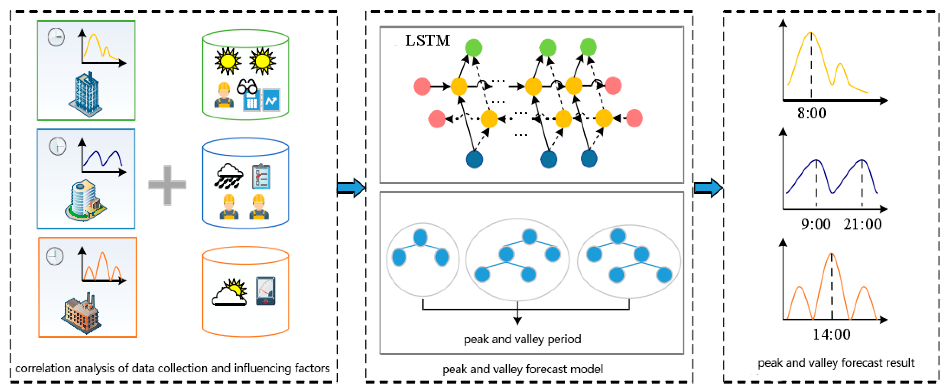
This research processes the 15 min electric-load data of the regional power grid to obtain the daily maximum (minimum) at peak-valley time. The temporal features and weather features are extracted, and the correlation test is carried out to screen out the feature sets whose correlation exceeds the threshold. The numerical forecasting model is established, and the time-segment classification model is further established and the parameters are adjusted. The load and weather characteristics of the previous two years are forecast, the forecasting results of the maximum (minimum) daily load and the arrival times in the next three months are provided, and the forecasting accuracy is analyzed.
The category variables with no order relation are coded independently to avoid the partial ordering of the variable values with no partial-order relation and to expand the characteristics. When screening features, the Pearson correlation coefficient is used to quantify the linear correlation, and the random forest is used to calculate the nonlinear correlation. It selected the indicators that reach the threshold to form the final feature set. The feature engineer not only considers fully the mining feature information, but also avoids dimensional disasters and multicollinearity problems through double screening.
In the medium-term load forecasting of daily peak and valley, this research applies the deep-learning model with long short-term memory (LSTM) and the relevant information of the sparrow search optimization algorithm (SSA) to accelerate the model convergence. The SSA was proposed in 2020; it mainly simulated the foraging and anti-predation behavior of the sparrow population [31]. This intelligent optimization algorithm is very novel, has strong optimization ability, and can greatly improve the efficiency of the forecasting model [32]. The SSA algorithm can research the global optimal solutions of load-forecasting results and can effectively prevent the situation in which the best expectation value found by the algorithm is always a local extreme value [33].
This paper proposes the LSTM-SSA-RF algorithm for the first time, which is applied to middle-term load forecasting. The innovation points of this paper have two aspects. First, the traditional algorithms with regression and neural networks have not had good results on middle-term load forecasting; the LSTM-SSA-RF algorithm has greater accuracy. The novel time-series forecasting algorithm and the novel intelligent optimization algorithm have been used in short-term load forecasting and not usually in middle-term load forecasting. Second, this paper adopts a new feature selection process with nonlinear correlation analysis.
This paper is organized as follows. Section 2 describes the considered methods and the algorithm framework. Section 3 provides the data processing, the characteristic engineering, and the forecasting results, which are reported and compared. Section 4 discusses the forecasting results. Section 5 draws some conclusions.
2. Methods and Algorithms
2.1. Single Algorithm Description of SSA-LSTM-RF
2.1.1. Long-Term and Short-Term Memory Network (LSTM)
LSTM is an excellent variant of the recurrent neural network (RNN), which can learn and preserve historical features for a long time. It can effectively solve the problem of gradient explosion and gradient disappearance by introducing a new internal state and gating mechanism [34]. LSTM can fully mine the temporal characteristics of data, with high forecasting accuracy, so it is widely used for electric-load forecasting—especially for medium-term and short-term forecasting [35]. Using the long-term dependence of LSTM learning data to measure the historical characteristic status improves the accuracy of forecasting.
LSTM adds or deletes cell-state information through a gate structure by introducing a memory structure and combining the output of the previous node at each time step. The LSTM’s basic unit and its specific calculation process are in Figure 1.
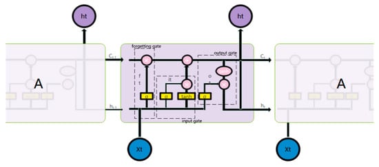
Figure 1.
Basic unit of LSTM network.
The forgetting gate is determined as follows:
The forgetting gate and the network structure parameters through the forgetting gate are adjusted through loss-function feedback during the training process. That is, according to the output of the previous stage and the input of the current stage, the forgotten part of the state of the moment is determined through the sigmoid function.
The input gate is determined as follows:
where is the input gate, controlling the network structure parameters through the input gate. That is, according to the output of the previous stage and the input of the current stage, the part that needs to be remembered for the state of the moment is determined through the sigmoid function, using the function to control the part of the alternative state added to the current state. Finally, you can obtain the current status, as follows:
The output gate is determined as follows:
where is the output gate, and is the network structure parameter through the output gate. The final output is the product of the part that needs to be output through the sigmoid function and the current state mapped by the function.
2.1.2. Sparrow Search Optimization Algorithm (SSA)
The LSTM model has high accuracy in medium-term load forecasting. Due to the large data set, this research also introduces the sparrow search algorithm (SSA) to accelerate the convergence. The SSA is a relatively novel intelligent optimization algorithm that seeks the optimal solution by simulating the foraging and anti-predation behavior of a sparrow population [36]. In the past two years, scholars have found through experiments that its convergence speed and accuracy are very good. Compared with particle swarm optimization (PSO), the SSA has a smaller probability of falling into a local optimum and stronger global search ability [37].
2.1.3. Random Forest Algorithm
Decision tree is a highly explanatory machine-learning model that conforms to the way people think and to business logic. However, considering the problems of local optimization and overfitting in regression using a single decision tree, we chose to use the random forest model [38]. Random forest is a very typical integrated learning technology, mainly using bagging technology. The random forest model has a good filtering effect on noise and outliers; it can overcome the overfitting problem, and it shows good parallelism and scalability in the classification of high-dimensional data. Based on its superior performance, the final choice was using random forest to forecast the peak-valley time [39].
2.2. Combined SSA-LSTM-RF Forecasting Algorithm
2.2.1. SSA-LSTM-RF Model Framework
In this research, we extracted the daily peak (valley) time from the 15 min interval load data of the power grid in the region, and combined them with the processed climate feature set and the trend feature set to form the peak forecast data set and the valley forecast data set. In order to forecast the peak and valley values of the daily load in the next three months and the corresponding arrival times, it was necessary to establish a medium-term load forecasting model and adjust the parameters to achieve the optimal forecasting accuracy. Based on the applicability analysis of the theoretical analysis part, this section mainly forecasts the load based on the LSTM model, optimizes it with the SSA algorithm, and then introduces random forest forecasting to reach the peak and valley times. The overall process is shown in Figure 2.
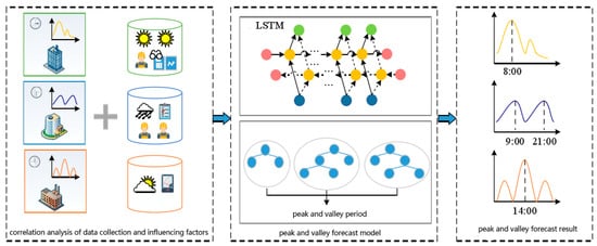
Figure 2.
Overall framework of the SSA-LSTM-RF model.
The overall process is shown in Figure 3, and the optimization process was as follows:
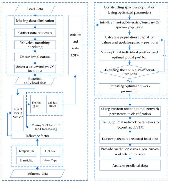
Figure 3.
Overall Process of SSA-LSTM-RF model.
- (1)
- Data process: Miss load data elimination, detect outlier data, process the data with wavelet smoothing and denoising, and select a time window of the load data.
- (2)
- Feature engineer: Create an alternative feature set of the load data and build a feature vector with influence factors.
- (3)
- Initialization: Initialize and train LSTM and determine the sparrow population size, the number of iterations, and the initial safety threshold based on the object to be optimized to initialize the SSA algorithm.
- (4)
- Fitness value: Determine the fitness value of each sparrow using the RMSE of the model forecasting value and sample data.
- (5)
- Update: Update the sparrow position, obtain the fitness value of the sparrow population, and save the optimal individual position and the global optimal position values in the population.
- (6)
- Iteration: Determine the iteration based on the loop conditions. If the conditions are met, exit the loop and return the individual optimal solution, which is the optimal parameter of the network structure. Otherwise, continue with step (5) of the loop.
- (7)
- Optimization result output: Assign values to the optimization object based on the optimal particles output by the SSA algorithm and use random forest optimal network parameters to classify and reconstruct the LSTM.
2.2.2. The SSA-LSTM Model Realizes Daily Peak and Valley Value Forecasting
In view of the complexity and diversity of medium-term electric load data, the SSA-LSTM model proposed in this section takes the historical electric load data as input and considers the impact of temperature, humidity, and date-type factors. The network model is constructed by modeling learning, and the internal change rules of network characteristics are also mined; The mapping, weighting, and learning parameter matrices are used to assign the corresponding weight value to the hidden state of LSTM network. At the same time, aiming at the problem of difficult selection of the model’s parameters, the sparrow search algorithm (SSA) is further proposed to realize the optimal selection of the model’s parameters [40].
SSA can be abstracted as an interactive model of bird explorers and followers who join the early warning mechanism (that is, there are some sparrows as scouts). Then, the position and the fitness value vector of the sparrows are set. The root mean square error (RMSE) is selected as the fitness function of the sparrow population.
The number of explorers and followers in the whole sparrow group is constant—that is, each additional follower will reduce one discoverer. The complete process of the algorithm is as follows [41].
Step 1: Initialize the population and set the maximum number of iterations.
Step 2: Update the discoverer location. At the beginning of each iteration, the explorer, as the best individual in the group, will obtain food first in the search process. During each iteration, the explorer’s position is updated as follows.
where represents the position of the sparrow in the dimension during the time iteration; represents a random number within the range of [0, 1]; indicates the alert value between [0, 1]; indicates the safety value between [0.5, 1]; and is a random number with normal distribution. When , it indicates that the environment is safe and the explorers are foraging in the area. Otherwise, it indicates that there are predators, and the scouts in the population need to send an alarm to signal the birds to go to the safe area for food.
Step 3: Update the follower position.
where represents the optimal position of fitness controlled by the explorer during the time iteration; indicates the global worst position; and is the population size. Each element of is randomly selected as 1 or −1, and ; takes 1 for each element. When , the follower has a low fitness value and needs to go to other areas for food.
Step 4: Randomly select the scout and update the position. The SSA indicates that there are individuals in each generation of the population with warning ability—that is, they can detect hazards. Generally, the range is 10–20%. The formula for updating the position of these sparrows is as follows.
where is a random number of standard normal distribution of load; indicates the current global optimal location; indicates the current fitness value of sparrow, and , respectively, represent the current best and worst fitness values; and represents a uniform random number of [–1, 1]. The setting of can prevents the denominator from being 0. When , it shows that the sparrow is at the center of the population and is randomly close to other sparrows. When , it shows that sparrows are vulnerable to predators in the remote areas of the whole population.
Step 5: When the number of iterations reaches the optimum value, stop the iteration.
In the above analysis, the SSA algorithm has been completed to optimize the parameters of LSTM model.
2.2.3. RF-LSTM Realizes Peak and Valley Time Forecasting
- A.
- Peak forecasting
In this research, the forecasting result of the daily peak was input into the random forest model, again as a feature. By dividing a time point every 15 min, 24 h were divided into 96 time points and numbered, and 96 time points were used as the classification target of the classifier.
According to the observation and analysis of the Pearson correlation coefficient, the peak time fluctuated greatly and was related to weather factors such as temperature, so the highest and lowest temperatures of the day were taken as the input features.
In addition, the peak time and the time were inseparable, with obvious seasonality and periodicity. The following time series characteristics were considered in this research:
- B.
- Valley forecasting
Because the valley time is relatively stable, it has little correlation with weather factors and it also has certain periodicity and seasonality. Therefore, the LSTM time-series model was selected to forecast the working electric data at 15 min intervals, and the valley time was extracted from the daily valley time in the results. The comparison showed that the effect of the LSTM model in forecasting the valley time was far from that of the random forest classifier.
2.3. Evaluation Indicators
In this research, RMSE, MAPE, MSE, and R-squared were selected as the evaluation indicators of the model [42].
Mean square error (MSE): MSE is the square of the difference between the real value and the forecasted value, and then the sum is averaged. The range is [0, +∞). When the forecasted value is completely consistent with the real value, it is equal to 0—that is, the perfect model. The greater the error, the greater the value.
Root mean square error (RMSE): RMSE is the square root of MSE. It measures the deviation between the forecasted value and the true value, and it is sensitive to the abnormal value in the data.
Mean absolute percentage error (MAPE): MAPE measures the percentage error between predicted results and actual observations. The range is [0, +∞), where 0% of MAPE indicates a perfect model, and more than 100% of MAPE indicates an inferior model.
R2 (R-squared) determination coefficient: R2 measures the degree of linear correlation between two variables. The numerator is the sum of the square difference between the real value and the forecasted value; The denominator is the sum of the square differences between the true value and the mean value. The value range of R-squared is [0, 1]: if it is closer to 0, the model fitting effect is very poor; if the result is 1, there is no error in the model. Generally speaking, the larger the R-squared, the better the fitting effect of the model.
3. Analysis and Results
3.1. Data Preprocessing
3.1.1. Handling Outlier Data
The existing methods for handling electric load data can generally be divided into three categories: statistical model methods, clustering model methods, and classification model methods. Statistical models describe the patterns and distributions of outlier data, compare similarities, and use outlier data indicators or criteria to construct one or more combination probability models. Clustering models can obtain classification results based on differences in load characteristics, effectively reflecting the overall characteristics of the load curve and detecting anomalies. Classification models often require a large amount of labeled information, and the actual application of abnormal samples is much smaller than that of normal samples, which can also lead to the problem of imbalanced sample distribution.
This research used the regional 15 min load data, industrial daily load data, and meteorological data. First, the standard deviation algorithm (k sigma) was used to test the outliers of the regional 15 min load data and the industrial daily load data and to set them as blank. Under the assumption of normal distribution (large samples can be regarded as normal distribution, approximately), the k sigma principle indicates that the probability of values outside the k times standard deviation of the average value is very small. Then, it checks the abnormal value of the 15 min load data of the area, selects k = 3, and sets 332 abnormal records.
3.1.2. Filling in Missing Values
Even though some of the technologies used in this research contained the existence of missing values, considering that different models have different means to deal with missing values, in order to ensure the accuracy of the solution, it was still necessary to fill in the missing values. In Figure 4, the data set was searched and it was found that only the regional 15 min load data and the industry daily load data had missing values (including the abnormal values that had been set to null). For this kind of numerical data, this research applied the linear interpolation algorithm to retain the local linear trend.
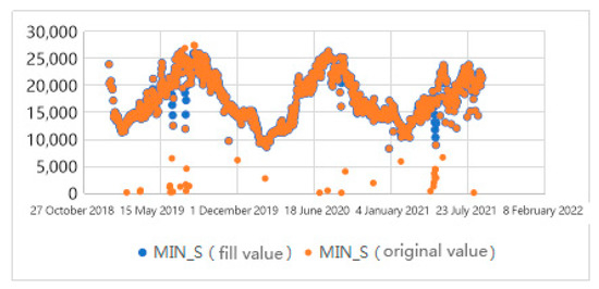
Figure 4.
Comparison of minimum daily load data before and after interpolation.
3.1.3. Data Processing by Type
The exploration data found that the “weather” characteristic format of meteorological data in the basic data was “weather 1/weather 2”, which could not be directly applied to numerical analysis. It was easy to lead to “dimension disaster” when using unique hot coding for expansion. A custom weather dictionary was selected, and each weather corresponded to the amount of illumination and precipitation, which was convenient for model training. Similarly, there were as many as 39 features of “wind and direction”, which were not directly coded. The wind characteristics were reserved.
Seasonal features were added to basic data. Because there was no order or difference between the values of a “season”, this research needed to use dummy variables and used the unique heat coding to expand the feature.
3.2. Characteristic Engineering
3.2.1. Creating an Alternative Feature Set
First, it was necessary to establish sufficient alternative feature sets. According to a large number of existing research bases, the main influencing factors of medium-term and short-term load are time-sequence factors, meteorological factors, and random interference factors, which consider the forward dependence of load and the historical load data. Due to the unforecastable nature of random interference factors, this research did not separately select random interference factors as characteristics; this is explained in the section on mutation-point analysis and policy-effect evaluation.
- (1)
- Time series factors included the month, the day ordinal of a month, the hour, the day ordinal of a year, the week ordinal of a year, the working day, holidays, the time period ordinal (divided by 3 h), the season ordinal (converted into a unique code), the beginning of a month, the end of a month, etc.
- (2)
- Meteorological factors included the maximum temperature, the minimum temperature, the temperature difference, the wind force, illumination, precipitation, etc.
- (3)
- Trend factors (historical load data) included the maximum (minimum) load of the previous day and the maximum (minimum) load of the previous week.
In considering the continuity of monthly data and hourly data, direct coding is not suitable. For example, 23 points and 0 points are similar in a practical sense, but direct coding can easily lead to a distance of 23 h. In order to avoid the discrepancy between the coding meaning and the actual meaning, in the regression analysis, this research cosined the monthly data (Formula (1)) and the hourly data (Formula (2)).
3.2.2. Feature Selection
Feature selection (FS) is an important problem in feature engineering. By eliminating redundant features and searching for the optimal feature subset, the efficiency of model solving is ultimately improved. This research mainly used the filter algorithm to filter the characteristics according to the correlation indicators in various statistical tests.
- (1)
- Linear correlation analysis: Pearson correlation coefficient
Pearson correlation coefficient is a typical indicator to measure the linear relationship between two variables. The calculation is relatively simple. The larger the coefficient, the stronger the linear correlation.
- (2)
- Nonlinear correlation analysis: random forest
Both the maximum mutual trust coefficient (MIC) and the Gini coefficient can be used to calculate nonlinear correlation. In this research, the feature selection algorithm based on random forest was used to select features by calculating the average reduction of the impurity of each feature. For classification, information gain was used. For regression, variance was used.
The nonlinear correlation coefficient of the regression model was calculated by random forest, and double screening was carried out.
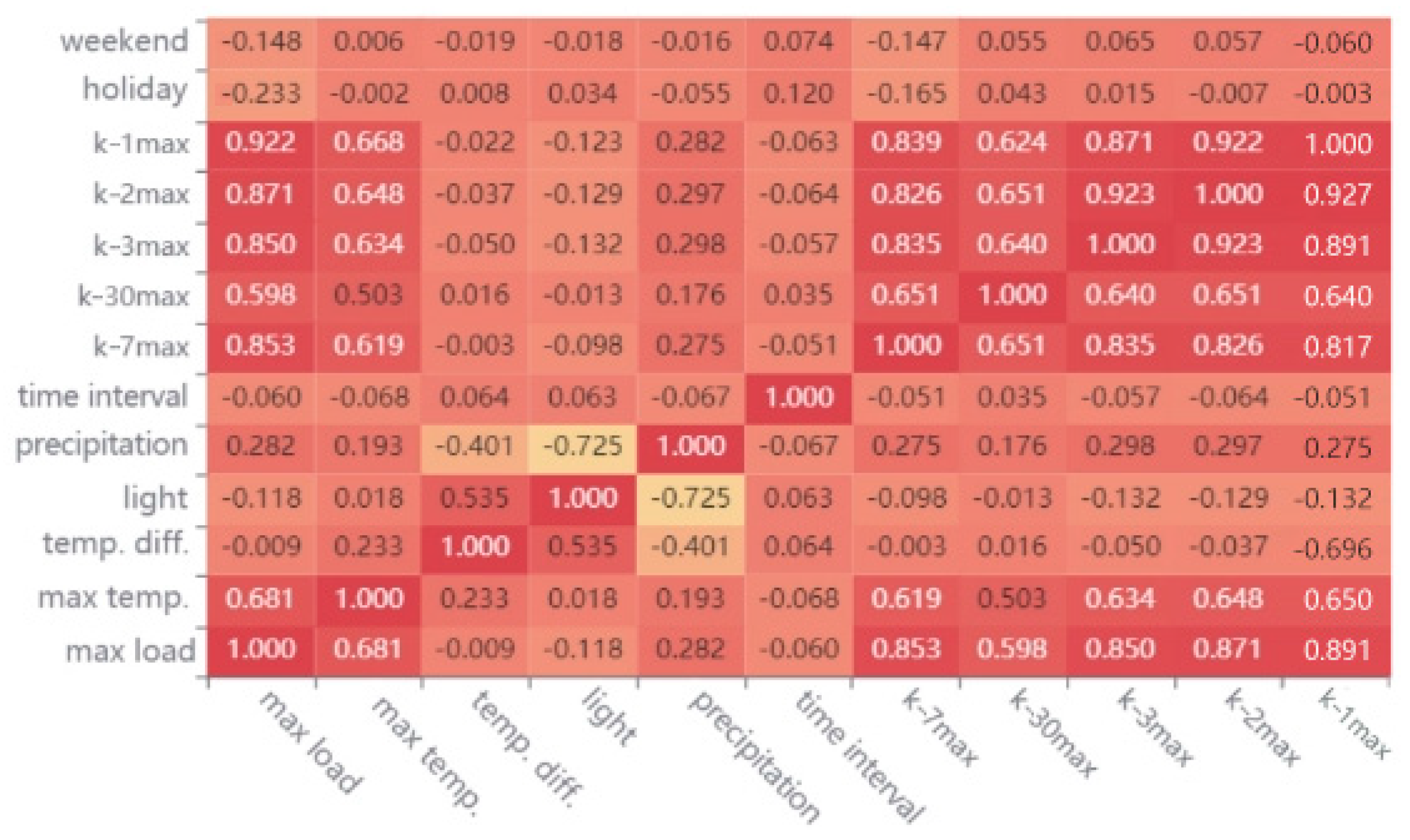
The results of feature screening in Figure 5 were based on the following:
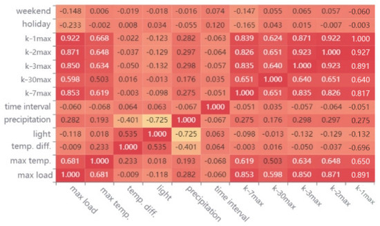
Figure 5.
Calculation results of Pearson correlation coefficient.
- (1)
- Peak value forecasting: The difference between the charge peaks and valleys of the previous day, the maximum temperature, the minimum temperature, the season, the light, the precipitation, the weekend/workday/holiday time point, the peak value of the previous day, the peak value of the previous 2 days, the peak value of the previous 5 days, the peak value of the previous 6 days, the peak value of the previous 7 days, and the peak value of the previous 30 days.
- (2)
- Valley value forecasting: The difference between the charge peaks and valleys of the previous day, the maximum temperature, the minimum temperature, the season, the valley value of the previous day, the valley value of the previous 2 days, the valley value of the previous 3 days, the valley value of the previous 7 days, and the valley value of the previous 30 days.
- (3)
- Forecasting of peak time: The forecasted peak, the maximum temperature, the minimum temperature, the light, the precipitation, whether it was a holiday, the season, the time point of the first day, the time point of the first 2 days, the time point of the first 5 days, the time point of the first 6 days, the time point of the first 7 days, and the time point of the first 30 days.
- (4)
- Forecasting of valley time: The time point of the first day, the time point of the first 2 days, the time point of the first 5 days, the time point of the first 6 days, the time point of the first 7 days, and the time point of the first 30 days.
3.3. Data Process Results of the SSA-LSTM-RF Algorithm
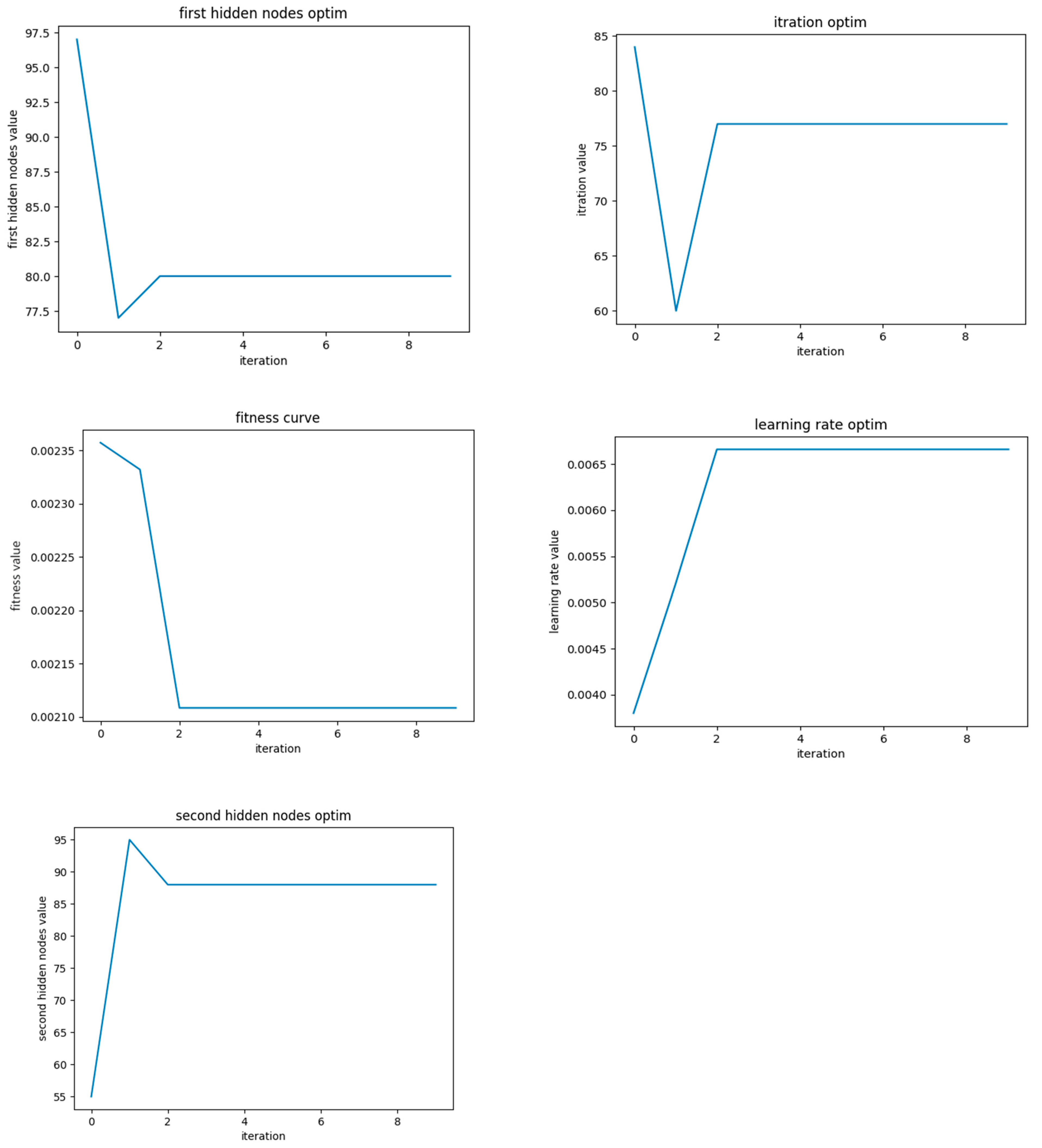
This research selected the number of neurons in the hidden layer of LSTM and included the first hidden nodes L1, the second hidden nodes L2, the iterations number iter, and the learning rate lr. These four key parameters that affected the performance of the LSTM model were taken as the optimization objects of the SSA.
The SSA-LSTM-RF optimization process in Figure 6 was as follows:
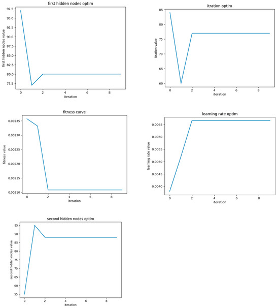
Figure 6.
Calculation results of SSA-LSTM-RF algorithm.
- (1)
- The number of neurons in the hidden layer of LSTM, included first hidden nodes L1, the second hidden nodes L2, the iterations number iter, and the learning rate lr were taken as the optimization objects, and constructed the parameter optimization range.
- (2)
- The individual fitness of sparrows was determined, and MSE was regarded as the fitness-evaluation function, which was the fitness curve value of the SSA algorithm.
- (3)
- The position information of sparrow individuals was calculated and updated to obtain fitness values. If the result was the global optimal fitness, then the optimal fitness in the current sparrow population of the individual position was saved; if not, update sparrow position was updated.
- (4)
- It was determined whether the number of iterations reached the upper limit. If so, the optimization process was exited and the returned optimal solution was saved. Otherwise, loop 3 was continued.
- (5)
- The optimized L1, L2, iter, and lr were substituted into the LSTM model with a random number.
- (6)
- The optimized model was used for forecasting.
As shown in Table 1, through 175 iterations, the learning rate reached 0.0060 and the hyperparameters received the optimization stations.

Table 1.
The results of the SSA for hyperparameters.
As shown in Figure 7, the optimization results of the SSA-LSTM-RF algorithm, shown in Figure 7a, were significantly better than those of the PSO-LSTM-RF algorithm, shown in Figure 7b, with higher convergence accuracy and relatively fewer iterations. The results also provided sufficient persuasiveness for the forecasting model established in this article to be used for medium- and short-term power-load forecasting.
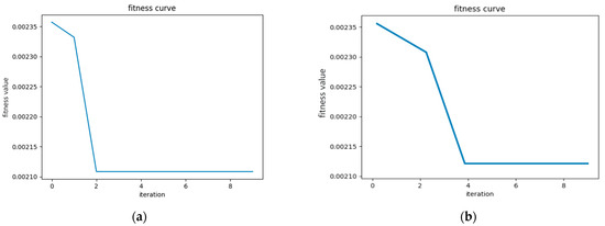
Figure 7.
Comparison of fitness curves between SSA-LSTM-RF and PSO-LSTM-RF. (a) SSA-LSTM-RF fitness curve. (b) PSO-LSTM-RF fitness curve.
3.4. Forecast Results of Minimum and Maximum Daily Loads
This research used the SSA-RF-LSTM model to evaluate the forecast results of the minimum daily load. The collected data of certain areas every 15 min were experimented with, using the SSA-RF-LSTM model.
This research forecast the daily peak and peak-valley times from the electric history-load data. This research carried out scenario forecasting based on the load and weather characteristics of the previous two years, provided the forecasted results of the minimum and maximum daily loads and arrival times for the next 300 days, and analyzed the forecasting accuracy.
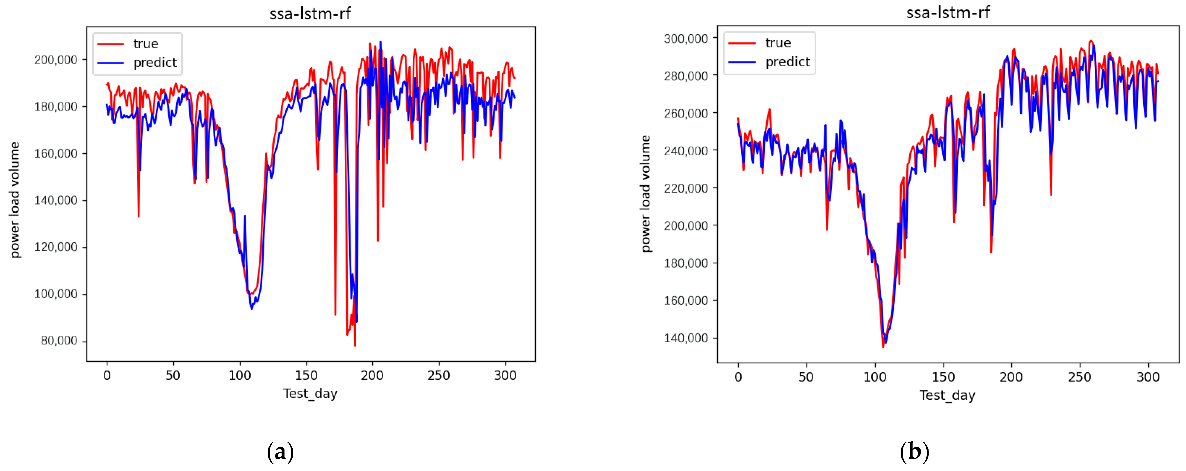
The experiment adapted the Python language with the sklearn packages to forecast results and with the Matplotlib packages to visualize the results. The experimental results are shown in Figure 8 and Figure 9.
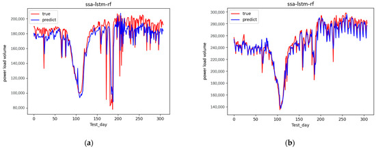
Figure 8.
Forecast results of minimum and maximum daily loads. (a) Forecast results of minimum daily load. (b) Forecast results of maximum daily load.
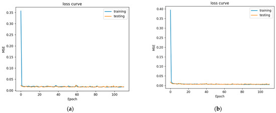
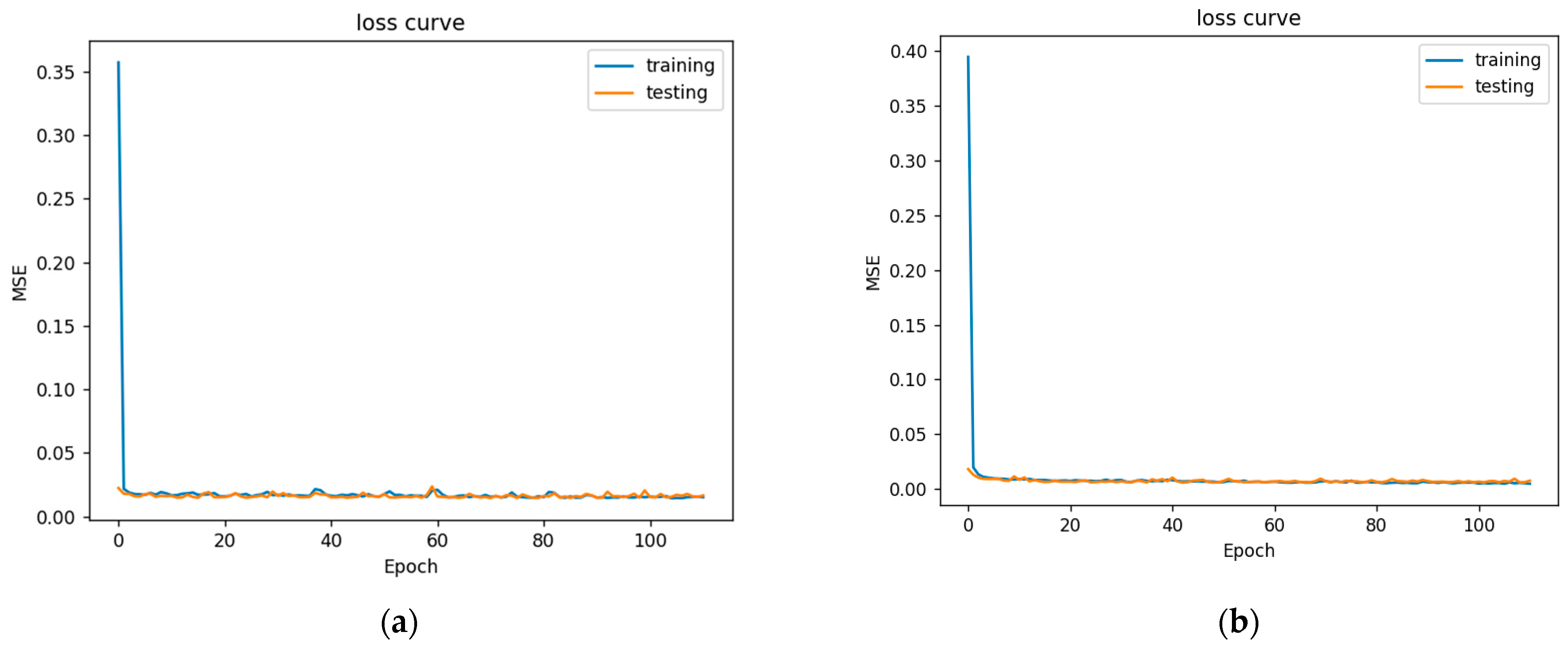
Figure 9.
Daily minimum and maximum loss curve. (a) Daily minimum loss curve. (b) Daily maximum loss curve.
In Figure 8, the forecast results of the minimum daily load are approximately the true minimum daily load in the 300 days. The forecast results of the maximum daily load were approximately the true maximum daily load in the 300 days. Relatively speaking, the maximum daily load was more approximate than the true minimum daily load with the true daily load.
In Figure 9 is a perfect loss curve graph. At the beginning of the training, the loss value decreased significantly, indicating that the learning rate was appropriate, and the gradient decline process was carried out. After learning to a certain stage, the loss curve tended to be stable, and the loss change was not as obvious as it was at the beginning. At the beginning of training, the loss value decreased rapidly, proving that the learning rate was appropriate. As the epoch increased, the learning rate gradually flattened out. The burrs in the curve were due to the relationship between batch sizes. The larger the batch size setting, the smaller the burrs.
3.5. Forecast Results of Daily Load with Different Algorithms and Steps
The LSTM network achieved the best performance by optimizing the super parameters through the SSA and RF. The MAPE, RMSE, and MSE of the forecasted values in the last two months of 2019 were accuracy and stability, respectively, which verified the accuracy and stability of the linear regression fitting ability of the model. See the annex for the results of scenario forecasting in Table 2.
Table 2.
The results of daily minimum and maximum load test.
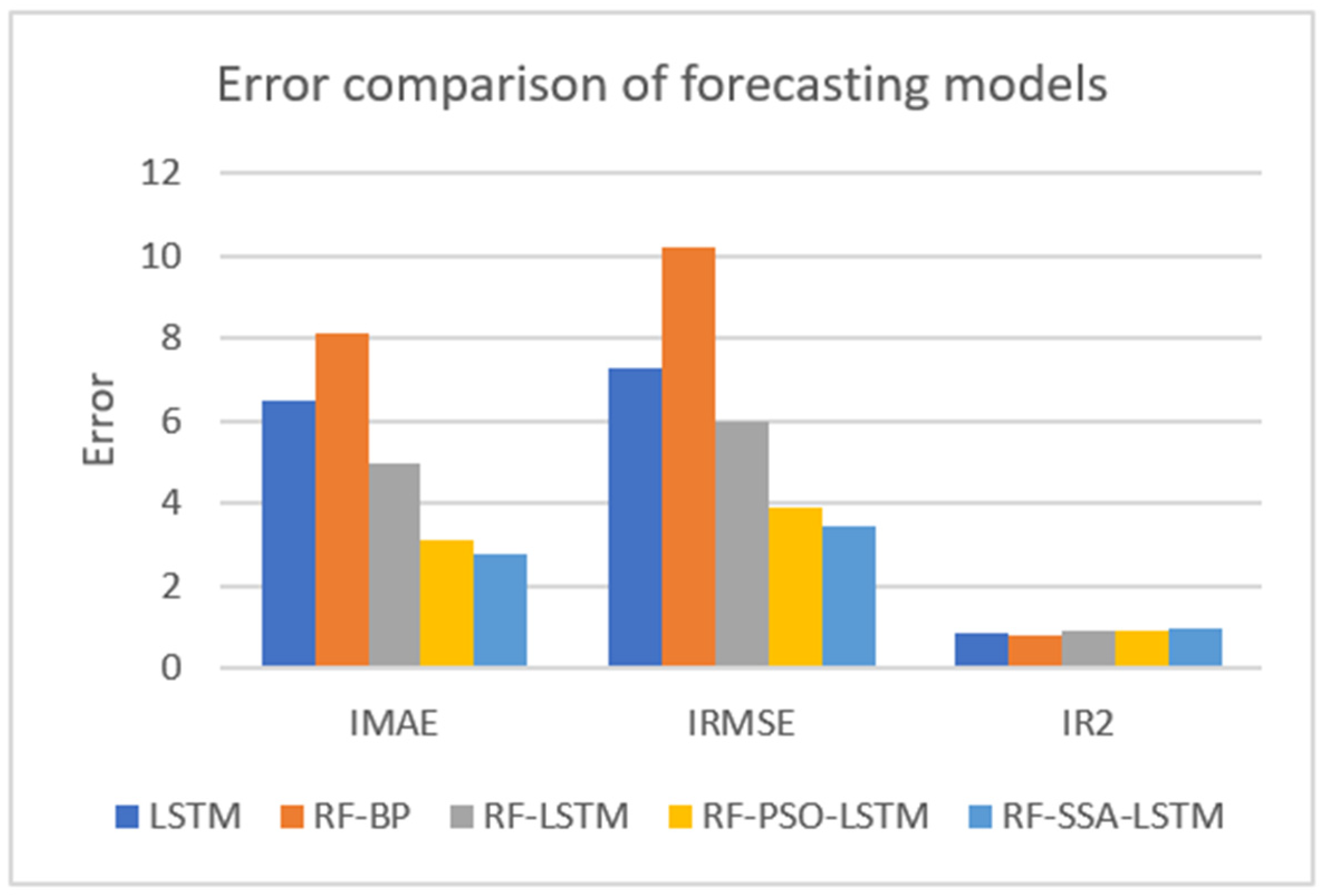
The collected data were experimented with these five models: LSTM, RF-BP, RF-LSTM, RF-PSO-LSTM, and RF-SSA-LSTM. The error comparison of the different forecasting models with 60 days is shown in Figure 10 and Table 3.
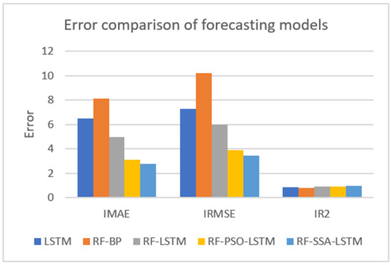
Figure 10.
Error comparison of different forecasting models.
Table 3.
Error comparison of different forecasting models.
From the results of the experiment, the smaller the result of IMAE, the better the forecasting effect; the smaller the result of IRMSE, the better the forecasting effect; and the greater the result of IR2, the better the forecasting effect. From the error comparison of the forecasting models, the effect of the RF-SSA-LSTM model was better than those of the LSTM, RF-BP, RF-LSTM, RF-PSO-LSTM, and RF-SSA-LSTM models.
The collected data were experimented with every 60 days, at 60 days, 120 days, 180 days, 240 days, and 300 days. The error comparison of the different forecasting times is shown in Figure 11 and Table 4.
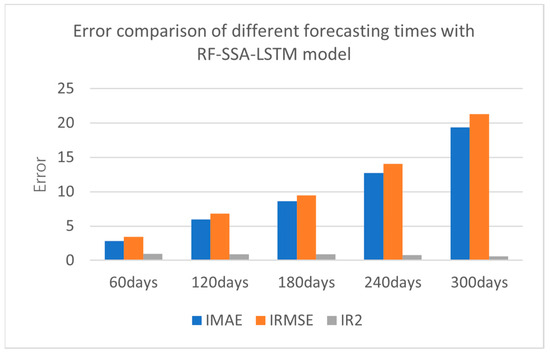
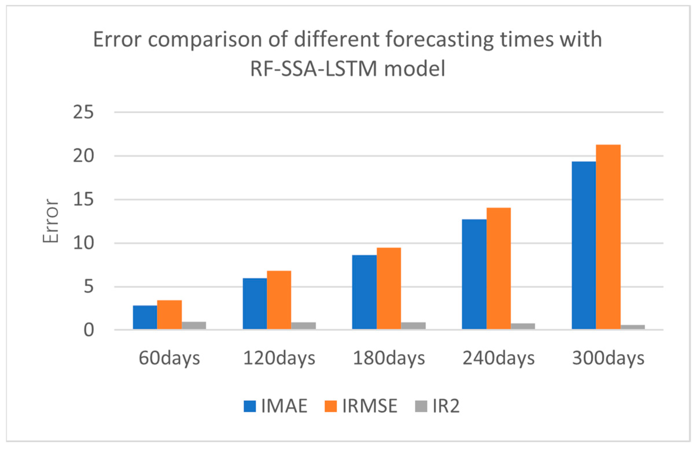
Figure 11.
Error comparison of different forecasting times with RF-SSA-LSTM model.
Table 4.
Error comparison of different forecasting times with RF-SSA-LSTM model.
From the results of experiment, the smaller the result of IMAE, the better the forecasting effect; the smaller the result of IRMSE, the better forecasting effect; and the greater the result of IR2, the better forecasting effect. From the error comparison of the different forecasting times, the best forecasting result was 60 days forecasting; as time goes by, it becomes lower and lower.
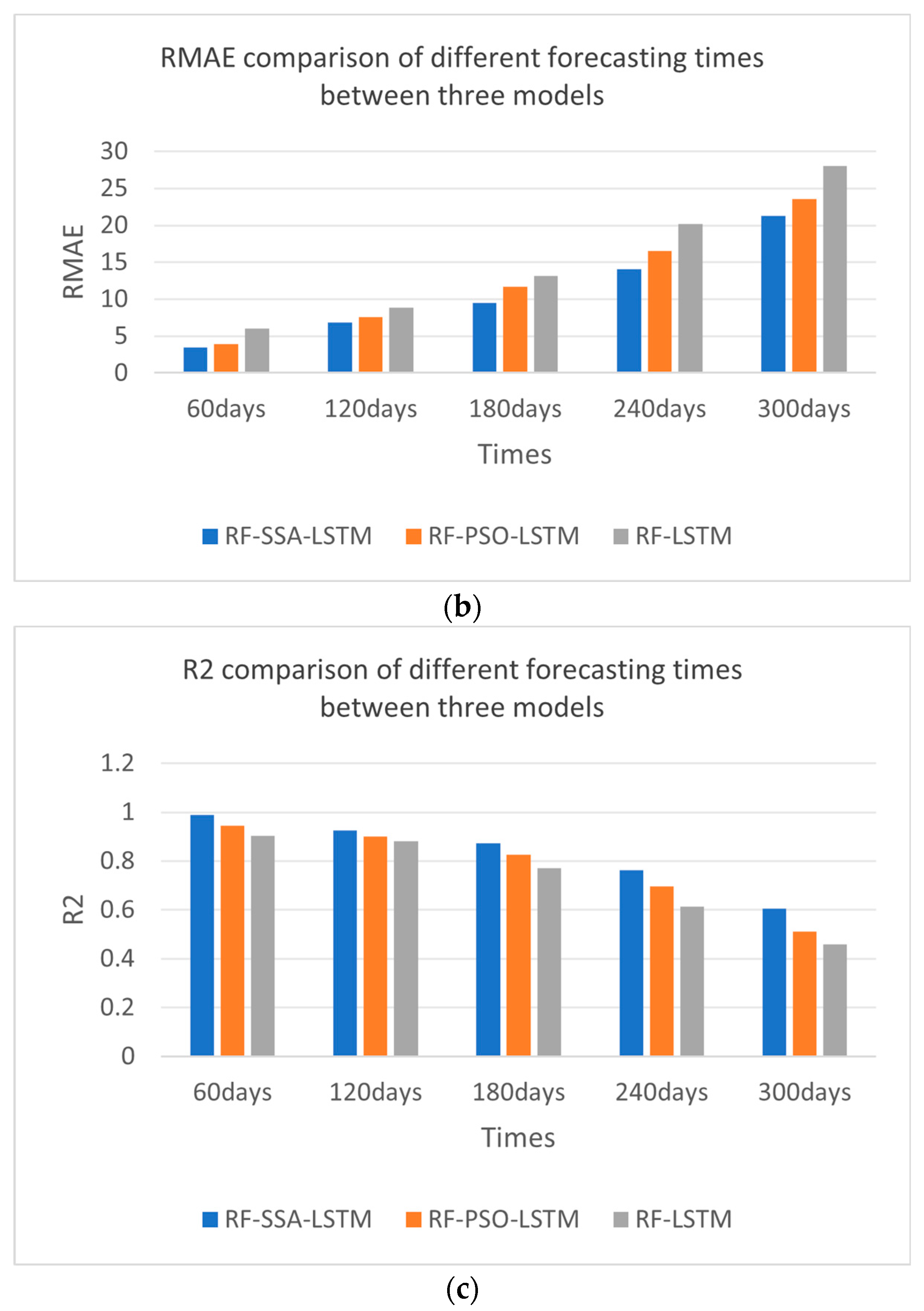
From the experimental results shown in Figure 12 and Table 5—the IMAE, IRMSE, and IR2 comparisons of different forecasting models—the effect of the RF-SSA-LSTM model was better than those of the RF-LSTM and RF-PSO-LSTM models, which were experimented with every 60 days, 120 days, 180 days, 240 days, and 300 days. From the error comparison of the different forecasting times, the best forecasting result was 60 days forecasting; as time goes by, the effect becomes worse and worse.
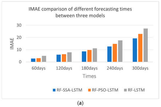
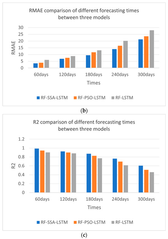
Figure 12.
Error comparison of different forecasting times between RF-SSA-LSTM, RF-PSO-LSTM and RF-LSTM models. (a) IMAE comparison of different prediction times. (b) RMAE comparison of different prediction times. (c) R2 comparison of different prediction times.
Table 5.
Error comparison of different forecasting times between RF-SSA-LSTM, RF-PSO-LSTM and RF-LSTM models.
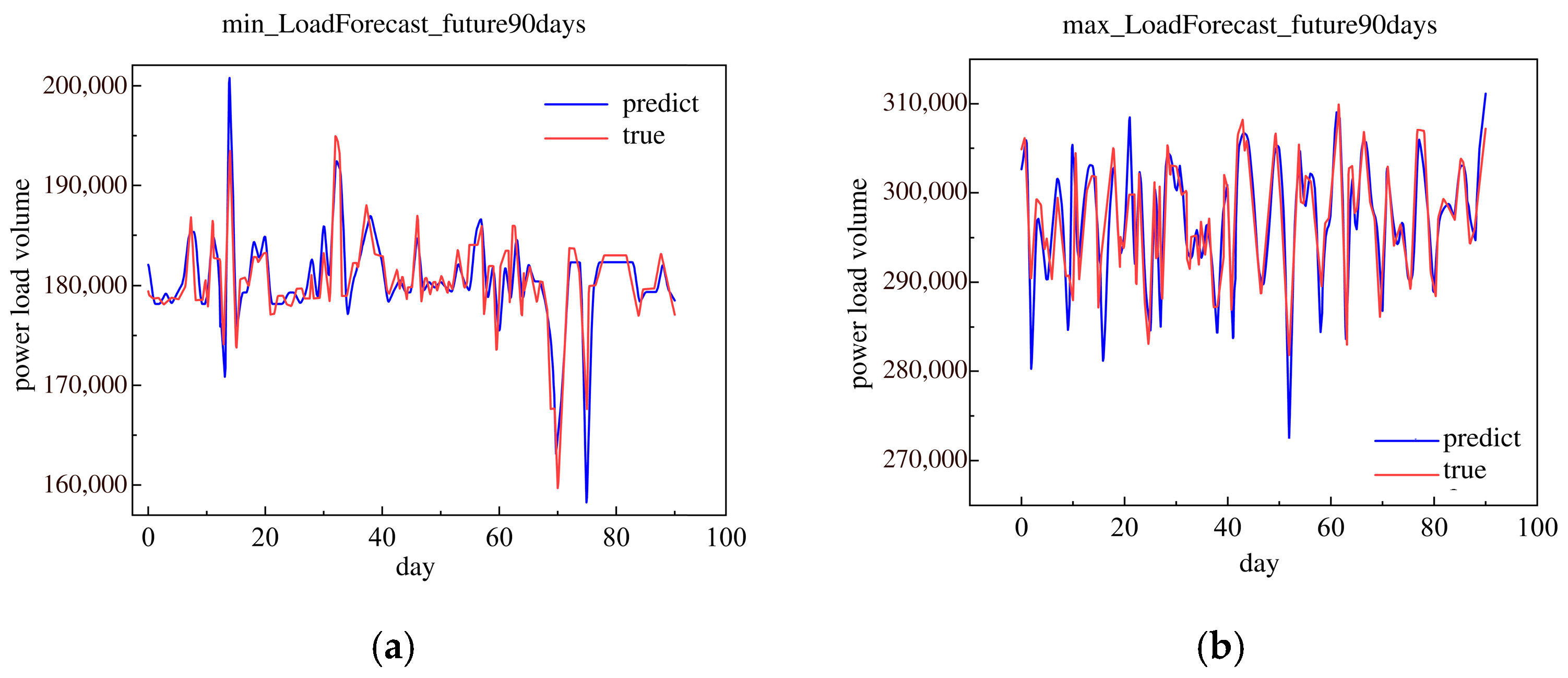
3.6. Forecast Evaluation of Minimum and Maximum Daily Load in the Future
This research used the historical load data in 2018 to forecast the future 90 days minimum and maximum daily loads. The future 90 day minimum and maximum daily loads are shown in Figure 13.
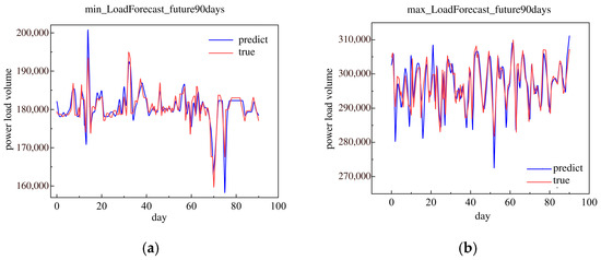
Figure 13.
The minimum and maximum of load forecast in the future 90 days in 2018. (a) Minimum load forecast in the future 90 days. (b) Maximum load forecast in the future 90 days.
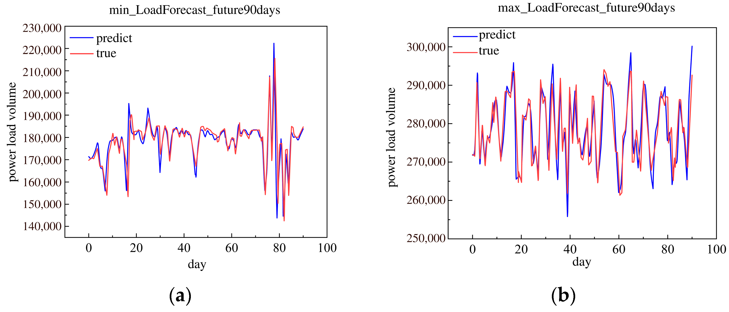
This research used the historical load data in 2019 to forecast the future 90 day minimum and maximum daily loads. The future 90 day minimum and maximum daily loads are shown in Figure 14.
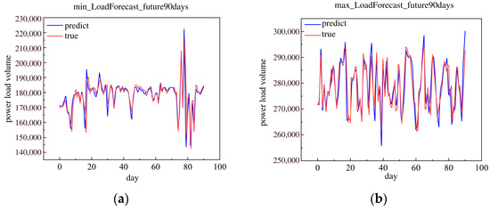
Figure 14.
The minimum and maximum of load forecast in the future 90 days in 2019. (a) Minimum load forecast in the future 90 days. (b) Maximum load forecast in the future 90 days.
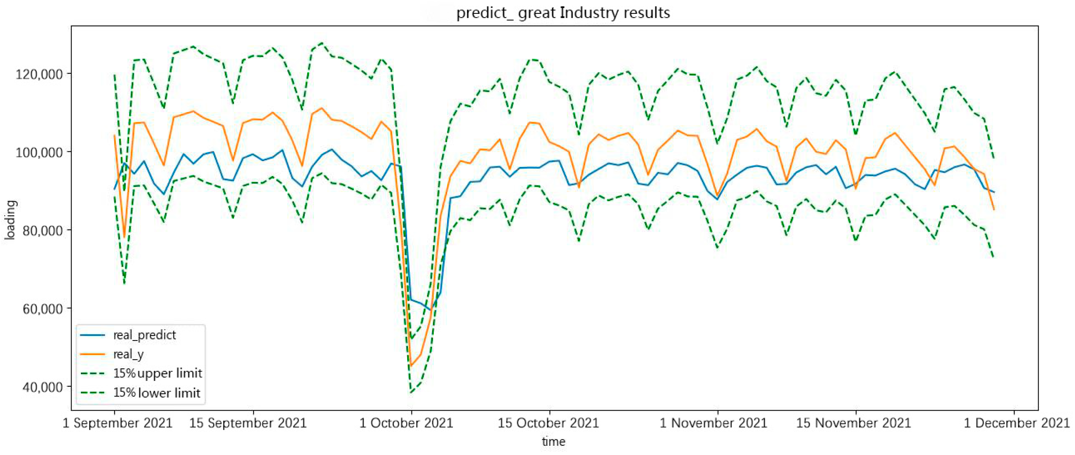
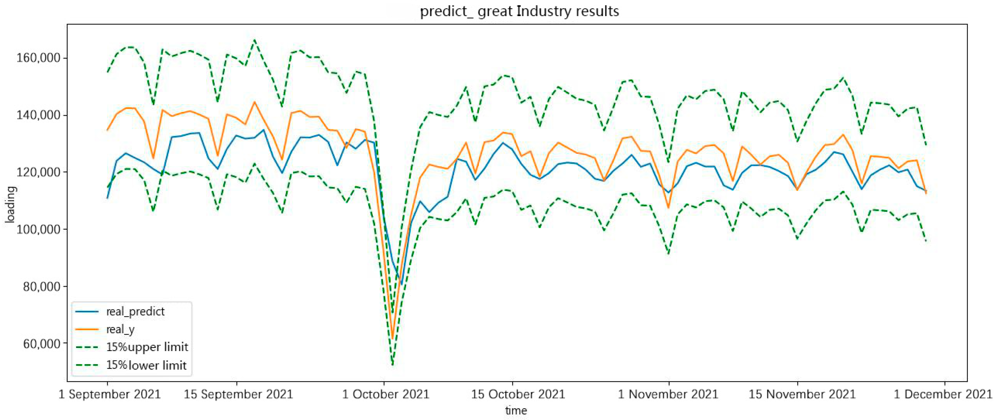
3.7. Forecast Evaluation of Minimum and Maximum Daily Load in Great Industry
Generally speaking, the classification of industries for electric-load forecasting by electricity-consumption characteristics includes great industries, non-general industries, general industries, and commerce. The trends of electric-load forecasting in different industries are different. This research proposes specific measures to forecast the evaluation of the future 90 days minimum and maximum daily load in a large industry.
In Figure 15 and Figure 16, the forecast results show the real value, the forecast result, the 15% upper limit, and the 15% lower limit. As shown in the forecast results, the holiday period had an important effect on the forecast results. During the holiday period in October, the forecast curve deviated from the original curve.
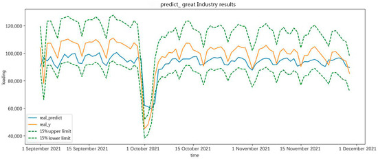
Figure 15.
The minimum of great-industry load forecasting in a future 90 days.
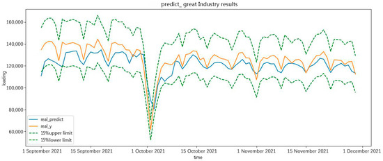
Figure 16.
The maximum of great-industry load forecasting in the future 90 days.
The forecast results are approximately the real value of minimum and maximum daily load in a great-industry load forecast in the future 90 days. The forecast results prove the effectiveness of the forecasting.
4. Discussion
This research first used Pearson correlation coefficient and random forest model to select features; Then, this research proposed the RF-SSA-LSTM daily peak-valley forecasting model. The model took the target value, the climate characteristics, the time series characteristics, and the historical trend characteristics as input to the LSTM network to obtain the daily-load peak and valley values. The super parameters of the LSTM network were optimized by the SSA algorithm and the global optimal solution was obtained.
This research provides a daily peak-valley electric-load forecasting based on RF, the SSA, and LSTM. This research shows that the forecasting outcomes of the RF-SSA-LSTM algorithm provide a considerable improvement, as shown in Figure 10 and Figure 11 and Table 2, Table 3 and Table 4. Additionally, the accuracy of daily peak-valley electric-load forecasting were compared with the fitness curves between RF-SSA-LSTM and RF-PSO-LSTM, as shown in Figure 8, and the fitness curves of LSTM, RF-BP, RF-LSTM, RF-PSO-LSTM, and RF-SSA-LSTM were compared. The forecast evaluation of the future 90 days with minimum and maximum daily loads was determined. In this research, the RF-SSA-LSTM algorithm was used to update the displacement forecasting model. It was demonstrated that the RF-SSA-LSTM algorithm has higher accuracy and greater stability than the other algorithms, such as RF-PSO-LSTM. The SSA algorithm can research the global optimal solutions better than the PSO algorithm. The RF-SSA-LSTM algorithm has greater accuracy than the other algorithms.
As the forecasting time step increases, the deviation between the electric-load forecasting results and the real values becomes more and more obvious, and the overall forecasting effect becomes worse. The forecasting results of 300 days were far inferior to those of 60 days, 120 days, 180 days, and 240 days. The longer the forecasting time, the poorer the forecasting of MAE, RMSE, and R2. However, the forecasting accuracy of this algorithm can also be further improved—for example, by using more precise data collection techniques to improve the accuracy of model forecasting.
Finally, the forecasting peak and valley values were also input into the random forest, as features to obtain the output of peak-valley time. The MAPE value of the SSA-LSTM-RF forecasting model was 1.5%, and the fitting ability was also good.
5. Conclusions
In summary, this research optimizes the LSTM displacement forecasting model using the SSA and RF algorithms to establish a preliminary displacement forecasting model for electric-load forecasting. The conclusions are as follows:
The environmental variables in electric-load forecasting are complex and nonlinear. This paper used the RF algorithm to weigh the environmental characteristic variables that affect electric-load forecasting. This research, analyzing and selecting feature variables with higher weights, reduced the computational power of the forecasting model, which was beneficial for improving the accuracy of the forecasting model. We searched for the optimal parameters of the LSTM model using the SSA search algorithm. Compared with commonly used grid search methods and PSO algorithms, the sparrow search algorithm has a simple structure and a high convergence rate, with both the global optimization ability of grid search and the local search ability of pattern search, forming complementary advantages. Through experimental comparison, it can be seen that the electric-load forecasting model based on RF-SSA-LSTM proposed in this article has higher forecasting accuracy and provides ideal performance for electric-load forecasting with different time steps.
With the development of deep-learning methods, this research should replace the RF method with deep-learning methods, such as XGBOOST and TCN. In addition to short-term and medium-term electric-load forecasting in a region, the medium-term and long-term electric-load forecasting focus on industry is extremely important for power-system planning and operation. The above research points should be the basis for future research recommendations.
Author Contributions
Conceptualization, S.S. and Z.C.; methodology, Y.W. and S.S.; software, Y.W.; validation, Y.W., S.S. and Z.C.; formal analysis, Y.W.; resources, Y.W., S.S. and Z.C.; data curation, Y.W.; writing—original draft preparation, Y.W.; writing—review and editing, Y.W., S.S. and Z.C; visualization, Y.W.; supervision, S.S. and Z.C. All authors have read and agreed to the published version of the manuscript.
Funding
This research received no external funding.
Data Availability Statement
The data presented in this study are available on request from the corresponding author. The data are not publicly available due to patient privacy.
Conflicts of Interest
The authors declare no conflict of interest.
Nomenclature
| LSTM | Long short-term memory |
| SSA | Sparrow search algorithm |
| RF | Random forest |
| PSO | Particle swarm optimization |
| MAE | Mean absolute error |
| MAPE | Mean absolute percentage error |
| MSE | Mean squared error |
| RMSE | Root mean squared error |
| R2 | Coefficient of determination |
References
- Erol-Kantarci, M.; Mouftah, H.T. Energy-efficient information and communication infrastructures in the smart grid: A survey on interactions and open issues. IEEE Commun. Surv. Tutor. 2015, 17, 179–197. [Google Scholar] [CrossRef]
- Boroojeni, K.G.; Amini, M.H.; Bahrami, S.; Iyengar, S.S.; Sarwat, A.I.; Karabasoglu, O. A novel multi-time-scale modeling for electric power demand forecasting: From short-term to medium-term horizon. Electr. Power Syst. Res. 2017, 142, 58–73. [Google Scholar] [CrossRef]
- Hong, T.; Fan, S. Probabilistic electric load forecasting: A tutorial review. Int. J. Forecast. 2016, 32, 914–938. [Google Scholar] [CrossRef]
- Raza, M.Q.; Khosravi, A. A review on artificial Intelligence based load demand forecasting techniques for smart grid and buildings. Renew. Sustain. Energy Rev. 2015, 50, 1352–1372. [Google Scholar]
- Gupta, V. An overview of different types of load forecasting methods and the factors affecting the load forecasting. Int. J. Res. Appl. Sci. Eng. Technol. 2017, 4, 729–733. [Google Scholar] [CrossRef]
- Yildiz, J.; Bilbao, I.; Sproul, A.B. A review and analysis of regression and machine learning models on commercial building electricity load forecasting. Renew. Sustain. Energy Rev. 2017, 73, 1104–1122. [Google Scholar] [CrossRef]
- Hippert, H.S.; Pedreira, C.E.; Souza, R.C. Neural networks for short-term load forecasting: A review and evaluation. IEEE Trans. Power Syst. 2001, 16, 44–55. [Google Scholar] [CrossRef]
- Singh, P.; Dwivedi, P. Integration of new evolutionary approach with artificial neural network for solving short term load forecast problem. Appl. Energy 2018, 217, 537–549. [Google Scholar] [CrossRef]
- Moon, J.; Park, J.; Hwang, E.; Jun, S. Forecasting power consumption for higher educational institutions based on machine learning. J. Supercomput. 2018, 74, 3778–3800. [Google Scholar] [CrossRef]
- Song, K.B.; Baek, Y.S.; Hong, D.H.; Jiang, G. Short-term load forecasting for the holidays using fuzzy linear regression algorithm. IEEE Trans. Power Syst. 2005, 20, 96–101. [Google Scholar] [CrossRef]
- Ceperic, E.; Ceperic, V.; Baric, A. A strategy for short-term load forecasting by support vector regression machines. IEEE Trans. Power Syst. 2013, 28, 4356–4364. [Google Scholar] [CrossRef]
- Wang, R.; Zhang, S.; Xiao, X.; Wang, Y. Short-term Load Forecasting of Multi-layer Long Short-term Memory Neural Network Considering Temperature Fuzziness. Electr. Power Autom. Equip. 2020, 40, 181–186. [Google Scholar]
- Lahouar, A.; Slama, J.B.H. Day-ahead load forecast using random forest and expert input selection. Energy Convers. Manag. 2015, 103, 1040–1051. [Google Scholar] [CrossRef]
- Abdoos, A.; Hemmati, M.; Abdoos, A.A. Short term load forecasting using a hybrid intelligent method. Knowl. Based Syst. 2015, 76, 139–147. [Google Scholar] [CrossRef]
- Dong, J.-R.; Zheng, C.-Y.; Kan, G.-Y.; Zhao, M.; Wen, J.; Yu, J. Applying the ensemble artificial neural network-based hybrid data-driven model to daily total load forecasting. Neural Comput. Appl. 2015, 26, 603–611. [Google Scholar] [CrossRef]
- Cecati, C.; Kolbusz, J.; Różycki, P.; Siano, P.; Wilamowski, B.M. A novel RBF training algorithm for short-term electric load forecasting and comparative studies. IEEE Trans. Ind. Electron. 2015, 10, 6519–6529. [Google Scholar] [CrossRef]
- Rutkowski, L.; Jaworski, M.; Pietruczuk, L.; Duda, P. The CART decision tree for mining data streams. Inf. Sci. 2014, 266, 1–15. [Google Scholar] [CrossRef]
- Han, M.; Tan, A.; Zhong, J. Application of Particle Swarm Optimization Combined with Long and Short-term Memory Networks for Short-term Load Forecasting. In Proceedings of the 2021 International Conference on Robotics Automation and Intelligent Control (ICRAIC 2021), Wuhan, China, 26–28 November 2021. [Google Scholar]
- Zhao, B.; Wang, Z.; Ji, W.; Gao, X.; Li, X. A Short-term power load forecasting Algorithm Based on Attention Mechanism of CNN-GRU. Power Syst. Technol. 2019, 43, 4370–4376. [Google Scholar]
- Lu, J.; Zhang, Q.; Yang, Z.; Tu, M.; Lu, J.; Peng, H. Short-term Load Forecasting Algorithm Based on CNN-LSTM Hybrid Neural Network Model. Autom. Electr. Power Syst. 2019, 43, 131–137. [Google Scholar]
- Xue, J. Research and Application of a Novel Swarm Intelligence Optimization Technique: Sparrow Search Algorithm. Master’s Thesis, Donghua University, Shanghai, China, 2020. [Google Scholar]
- Mao, Q.; Zhang, Q. Improved Sparrow Algorithm Combining Cauchy Mutation and Opposition-based Learning. J. Front. Comput. Sci. Technol. 2021, 15, 1155–1164. [Google Scholar]
- Zhu, J.; Liu, S.; Fan, N.; Shen, X.; Guo, X. A Short-term power load forecasting Algorithm Based on LSTM Neural Network. China New Telecommun. 2021, 23, 167–168. [Google Scholar]
- Tan, M.; Yuan, S.; Li, S.; Su, Y.; Li, H.; He, F. Ultra-short-term industrial power demand forecasting using LSTM based hybrid ensemble learning. IEEE Trans. Power Syst. 2019, 35, 2937–2948. [Google Scholar] [CrossRef]
- Tian, H.; Zhang, Z.; Yu, D. Research on Multi-load Short-term Forecasting of Regional Integrated Energy System Based on Improved LSTM. Proc. CSU-EPSA 2021, 33, 130–137. [Google Scholar]
- Qing, X.; Niu, Y. Hourly day-ahead solar irradiance prediction using weather forecasts by LSTM. Energy 2018, 148, 461–468. [Google Scholar] [CrossRef]
- Zhang, J. Research and Analysis of Short-term Load Forecasting Based on Adaptive K-means and DNN. Electron. Meas. Technol. 2020, 43, 58–61. [Google Scholar]
- Liu, B. Research of Short-Term Power load Forecasting Based on PSO-LSTM Algorithm. Master’s Thesis, Jilin University, Changchun, China, 2020. [Google Scholar]
- Liu, K.; Ruan, J.; Zhao, X.; Liu, G. Short-term Load Forecasting Algorithm Based on Sparrow Search Optimized Attention-GRU. Proc. CSU-EPSA 2022, 34, 1–9. [Google Scholar]
- Huang, Z.; Huang, J.; Min, J. SSA-LSTM: Short-Term Photovoltaic Power Prediction Based on Feature Matching. Energies 2022, 15, 7806. [Google Scholar] [CrossRef]
- Yang, H.; Zhang, Q. An Adaptive Chaos Immune Optimization Algorithm with Mutative Scale and Its Application. Control Theory Appl. 2009, 26, 1069–1074. [Google Scholar]
- Liu, J.; Yuan, M.; Zuo, F. Global Search-oriented Adaptive Leader Salp Swarm Algorithm. Control Decis 2021, 36, 2152–2160. [Google Scholar]
- Han, M.; Zhong, J.; Sang, P.; Liao, H.; Tan, A. A Combined Model Incorporating Improved SSA and LSTM Algorithms for Short-Term Load Forecasting. Electronics 2022, 11, 1835. [Google Scholar] [CrossRef]
- Kong, W.; Dong, Z.Y.; Jia, Y.; Hill, D.J.; Xu, Y.; Zhang, Y. Short-term residential load forecasting based on LSTM recurrent neural network. IEEE Trans. Smart Grid. 2017, 10, 841–851. [Google Scholar] [CrossRef]
- Wang, S.; Wang, X.; Wang, S.; Wang, D. Bi-directional long short-term memory method based on attention mechanism and rolling update for short-term load forecasting. Int. J. Electr. Power Energy Syst. 2019, 109, 470–479. [Google Scholar] [CrossRef]
- Raza, M.Q.; Mithulananthan, N.; Li, J.; Lee, K.Y. Multivariate ensemble forecast framework for demand forecasting of anomalous days. IEEE Trans. Sustain. Energy 2018, 11, 27–36. [Google Scholar] [CrossRef]
- Liu, H.; Mi, X.; Li, Y. Smart multi-step deep learning model for wind speed forecasting based on variational mode decomposition, singular spectrum analysis, LSTM network and ELM. Energy Convers. Manag. 2018, 8, 54–64. [Google Scholar] [CrossRef]
- Kim, S.; Ko, B.C. Building deep random ferns without backpropagation. IEEE Access 2020, 8, 8533–8542. [Google Scholar] [CrossRef]
- Oshiro, T.M.; Perez, P.S.; Baranauskas, J.A. How many trees in a random forest? In Proceedings of the International Conference on Machine Learning and Data Mining in Pattern Recognition, Berlin, Germany, 13–20 July 2012; Volume 1, pp. 154–168. [Google Scholar]
- Cheng, J.; Zhang, N.; Wang, Y.; Kang, C.; Zhu, W.; Luo, M.; Que, H. Evaluating the spatial correlations of multi-area load forecasting errors. In Proceedings of the 2016 International Conference on Probabilistic Methods Applied to Power Systems (PMAPS), Beijing, China, 16–20 October 2016; Volume 1, pp. 1–6. [Google Scholar]
- Al Mamun, A.; Sohel, M.; Mohammad, N.; Sunny, M.S.H.; Dipta, D.R.; Hossain, E. A comprehensive review of the load forecasting techniques using single and hybrid forecastive models. IEEE Access 2020, 8, 134911–134939. [Google Scholar] [CrossRef]
- Kong, X.; Zheng, F.; Zhijun, E.; Cao, J.; Wang, X. Short-term Load Forecasting Based on Deep Belief Network. Autom. Electr. Power Syst. 2018, 42, 133–139. [Google Scholar]


Disclaimer/Publisher’s Note: The statements, opinions and data contained in all publications are solely those of the individual author(s) and contributor(s) and not of MDPI and/or the editor(s). MDPI and/or the editor(s) disclaim responsibility for any injury to people or property resulting from any ideas, methods, instructions or products referred to in the content. |
© 2023 by the authors. Licensee MDPI, Basel, Switzerland. This article is an open access article distributed under the terms and conditions of the Creative Commons Attribution (CC BY) license (https://creativecommons.org/licenses/by/4.0/).