Abstract
In coal seam gas (CSG) coproduction wells, due to the different production pressures of CSG production layer at different depths, the interlayer interference in wellbore seriously affects the gas production of a coproduction well. To effectively suppress the interlayer interference of the wellbore, a wellbore pressure distribution method for a two-layer coproduction well is proposed. Based on the analysis of the factors influencing the flow pressure distribution in the wellbore of two-layer coproduction wells, a method of coproduction flow pressure adjustment by regulating the wellhead pressure and the depth of the dynamic fluid level was established in this paper. The results show that wellhead pressure can directly affect the production pressure of two layers. The variation in layer 1 output mainly affects the pressure difference between the wellhead pressure and the pressure at the depth of layer 1, which has little effect on the pressure difference between layer 1 and 2. An increase in gas production from layer 2 would not only cause a pressure increase in layer 1, but also result in a reduction of the production pressure at layer 2. The maximum pressure gradient of the gas section is 0.14 MPa/100 m, and the pressure gradient of the gas–liquid section is 0.53–1.0 MPa/100 m.
1. Introduction
As unconventional natural gas, CSG has gradually become a trending topic in gas resource development. As the development of CSG resources has globally accelerated in recent years [1,2], the countries that are making great efforts to develop CSG exploitation include the United States, Australia, Canada, and China, with some fields already in commercial production [3]. Areas of vertical distribution with multiple potential production layers are currently discovered in the Ordos Basin, Qinshui Basin, Eastern Yunnan and western Guizhou in China [4,5,6,7,8]. Similar areas are also found in the United States, Australia and Canada, such as the San Juan Basin [9,10], Black Warrior Basin [11,12], Powder River Basin [13,14], Horseshoe Canyon Basin [15,16], and Bowen-Surat Basin [17,18].
Much attention has been focused on the multilayer coproduction of CSG wells. A multibranch U-shaped well was proposed for two coal seams in one well, which can provide single-layer or two-layer coproduction [19]. Notable progress has been made in physical experiments for multilayer CSG coproduction. The effects of reservoir permeability [1,20], bottom hole pressure [21,22], and coal seam depth [23] on the coproduction have been studied. The difference in reservoir geological properties is a fundamental factor affecting coproduction. While the pressure and fluid flow in the wellbore also affect coproduction, and the interlayer interference coefficient has been proposed to avoid interlayer interference [24,25,26,27,28,29,30]. These results have been verified in field CSG coproduction. However, the current multilayer coproduction efforts have not achieved the ideal result (both layers can produce, and the coproduction is greater than that of a single layer) due to the strong interlayer interference in the wellbore. The effective suppression of interlayer interference in a wellbore remains a challenge for the further development of CSG coproduction.
Due to water production from the CSG layer, the annular space between the tubing and casing is in a gas-liquid two-phase flow state during the coproduction, and there is a dynamic liquid surface [21,31]. The pressure distribution influences the pressure at the depth of different production layers in the wellbore. To solve the calculation of pressure distribution in the annular space, many experimental and theoretical studies have been conducted in recent decades. Sadatomi et al. established a calculation method for the frictional pressure difference of air-water two-phase flow by studying the two phases in the vertical annular space [32]. Hasan and Kabir established a calculation model of the void ratio when the annulus is in bubble flow and slug flow by theoretical and experimental analysis, which can facilitate the calculation of bottom hole pressure (BHP) in pumping wells and the calculation of wellbore pressure for pumping unit well [33]. Kelessidis and Dukler studied the gas-liquid two-phase flow in concentric and eccentric annular spaces and established a basis for determining the flow patterns in concentric and eccentric annuli [34]. Papadimitriou and Shoham studied the case of net-zero liquid flow in the annulus and established a model based on experiments for the bottom pressure in the annulus of a pumping well with net-zero liquid flow [35]. Antonio and Time developed a steady-state model for the pressure drop in concentric annular air–liquid two-phase flow [36]. An, H.-J., et al. studied the effect of liquid viscosity on the pressure drop of gas–liquid two-phase flow at a net-zero liquid flow rate [37].
Compared to single-layer production wells, multilayer coproduction wells have more significant development advantages, which can effectively reduce production costs and increase total gas production from a single well [38,39,40]. The long-term and stable gas production from multilayer CSG coproduction wells has become a technical challenge for coproduction wells. Compared to single-layer production, two production layers at different depths in coproduction wells have different pressures [24]. The fluids from the two layers entering the wellbore cause interlayer interference in the wellbore, which simultaneously affects the gas production capacity of the two production layers during coproduction [41]. Due to interlayer interference, the production capacity of some coproducing gas wells is even lower than that of single-layer production gas wells.
In the case of multilayer coproduction, the wellbore pressure varies at different depths (output pressure for each layer increases with depth). The production status of a single layer is influenced by the pressure at the depth of that layer in the wellbore [41]. Unlike the dry coal seams in the Alberta Basin and Surat-Bowen Basin, the CSG wells in the Ordos Basin and Eastern Yunnan and Western Guizhou Blocks in China have the problem of water production. Reasonable multilayer combination schemes for different block characteristics can effectively reduce interlayer interference in coproduction [31,39,42]. Moreover, due to the presence of multilayer gas systems, there is strong interlayer interference in existing multilayer coproduction wellbores. Effective regulation of the wellbore pressure distribution becomes the key to reasonably controlling the production pressure for both layers. A method to suppress interlayer interference in the wellbore is urgently needed for water-producing coproduction wells. To solve this problem, the key factors influencing the interlayer production pressure difference in the coproduction wellbore were investigated by analyzing the flow pattern of drainage in coproduction wells. A method was proposed to reasonably regulate the production pressure of the two combined production layers by controlling the wellhead pressure and the depth of the dynamic fluid surface. Furthermore, this method can effectively suppress interlayer interference between two layers.
The rest of the paper is organized as follows: in Section 2, the output model of two layers of CSG coproduction and the basic requirements of coproduction pressure distribution are investigated. In Section 3, the method of the coproduction well pressure distribution calculation is presented. Fifteen sets of physical experiments for CSG coproduction were designed and conducted in Section 4. Finally, The results of theoretical analysis and experiments and discussions are in Section 5.
2. Methods
2.1. Production Output and Wellbore Pressure Distribution
According to CSG and conventional natural gas production capacity research [43,44], the capacity equation of the production layer has the following form:
where: qg is the daily gas
production of a gas well, m3/d; k is the permeability of the
CSG reservoir, m2; H is the thickness of the coal seam, m; N
is the gas content of the coal seam, m3/t; pr is
the original layer pressure, MPa; pi is the wellbore pressure
at the depth of production layer i, where i = 1, 2, MPa; μ
is the viscosity of the fluids, mPa·s; Pji is the pressure at
the beginning of desorption of coalbed methane for layer i, MPa; S
is the surface skin of the wellbore; A and B are the laminar flow
coefficients and turbulence coefficients, which can be solved based on well
test data; C is the gas production index, which is related to the
permeability thickness of the production layer, the viscosity of the produced
gas and the bottom of the well’s conditions, 104 m3/d(MPa)−2n;
n is the gas percolation index and n = 1 for linear percolation;
When the fluid percolation rate is large or multiphase percolation occurs, n
< 1.
To ensure that both layers can produce normally, the pressure distribution in the wellbore should be:
where Pri is the original stratigraphic pressure of gas production layer i, MPa; Ptf is the pressure in the annulus at the wellhead, MPa; Pwf1 is the pressure in the annulus at the depth of the layer 1, MPa; Pwf2 is the pressure in the annulus at the depth of layer 2, MPa.
Especially for the desorption production of coalbed methane (CBM):
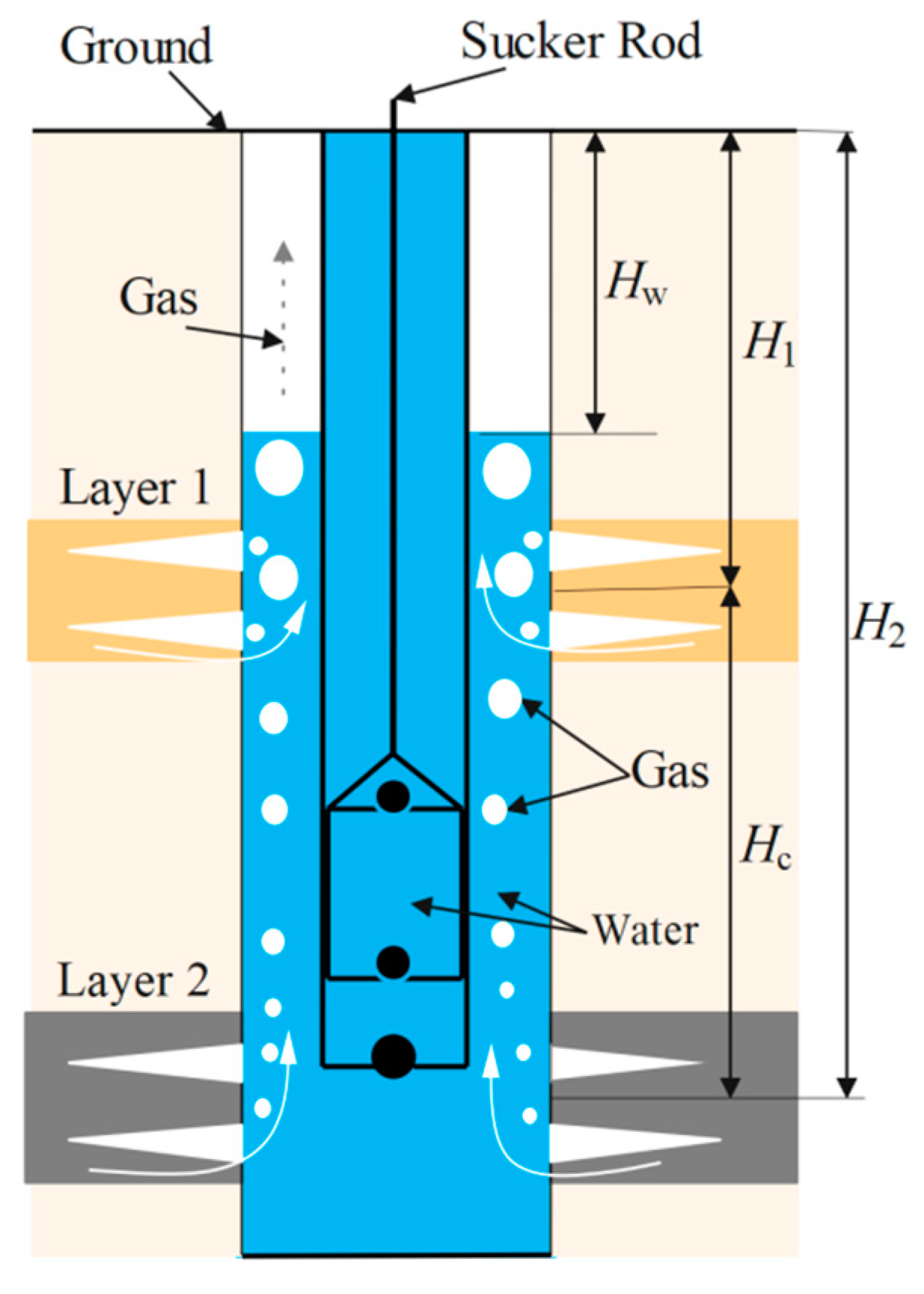
To coordinate the production of each layer in multilayer coproduction wells, a detailed study of the pressure distribution in the coproduction wellbore is needed. In this paper, as gas and water flow out from the two layers, an artificial lift device is used for drainage. Water from the layer accumulates in the annulus, which is lifted upward by an artificial lift pump, and then passes through the tubing to the ground. The gas produced from the producing layers enters the wellbore and flows through the annulus of the tubing and casing to the wellhead for output. A two-layer model with distance Hc is supposed to simplify the pressure distribution in the CSG wellbore instead of a multilayer model. The wellbore annulus of the CSG gas well is the three-dimensional annular space, and the wellbore is illustrated in the form of a cross-section in order to clearly express the distribution of fluids in the wellbore. Furthermore, the upper CSG layer is named layer 1, and the lower layer is layer 2, as shown in Figure 1.
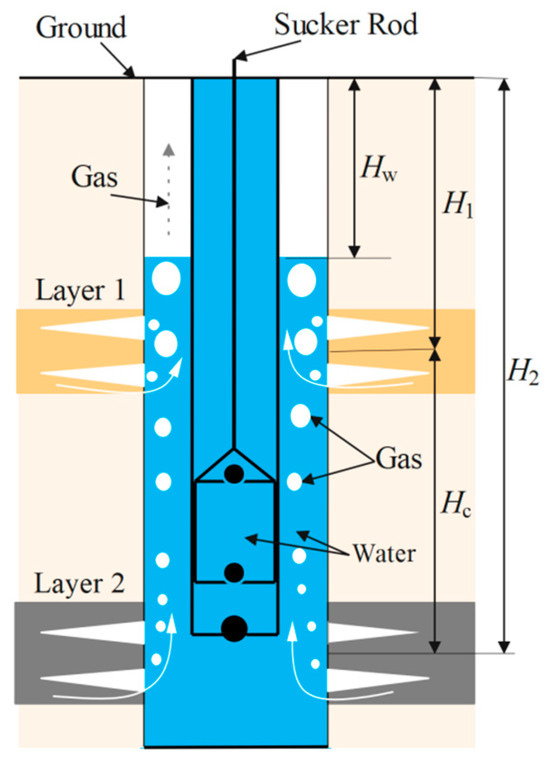
Figure 1.
Structure of a two-layer coproduction CSG well.
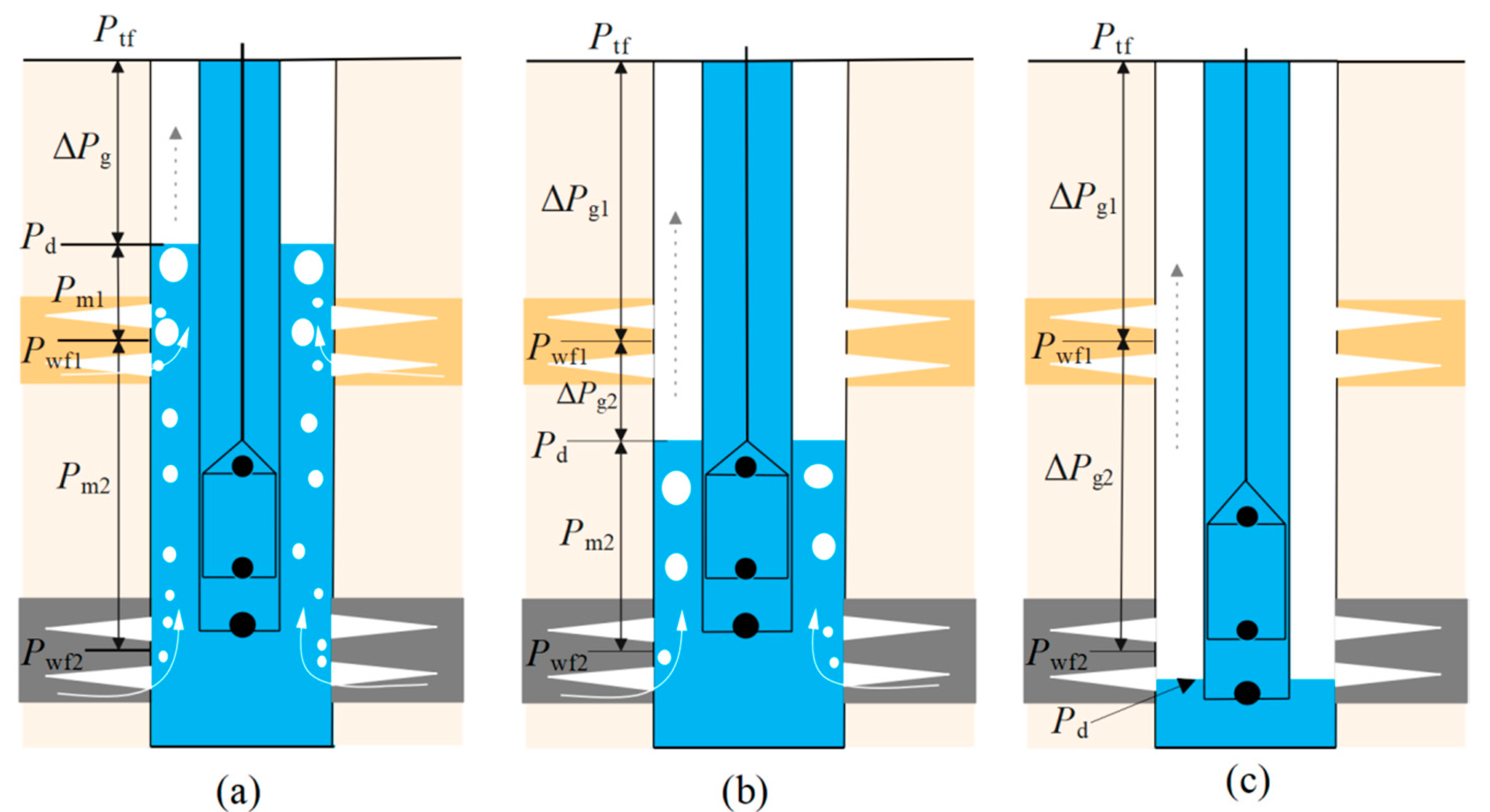
The gas in the wellbore below the dynamic liquid level flows up in the water as a bubble or slug flow. The gas above the dynamic liquid level in the wellbore annulus is a single-phase flow. The dynamic fluid level position in the wellbore varies. As shown in Figure 2a–c, influenced by dynamic fluid level depth in the wellbore the pressure relationship for each layer is as follows:
where: Hw is the distance from the dynamic fluid level in the wellbore to the ground, m; H1 is the distance from layer 1 to the ground, m; H2 is the distance from layer 2 to the ground, m; is the total pressure difference of the gas flow in the annulus, as shown in Figure 2a, MPa; is the pressure difference of the gas flow in the annulus at a depth of H1 to the ground, as shown in Figure 2b,c, MPa; is the pressure drop of the gas flow in the annulus at a depth of Hw to H1, as shown in Figure 2b,c, MPa; is the pressure drop in gas-liquid mixing zone between the dynamic fluid level and layer 1, as shown in Figure 2a, MPa; and is the pressure drop in gas-liquid mixing zone between layer 1 and layer 2 as shown in Figure 2a,b, MPa.
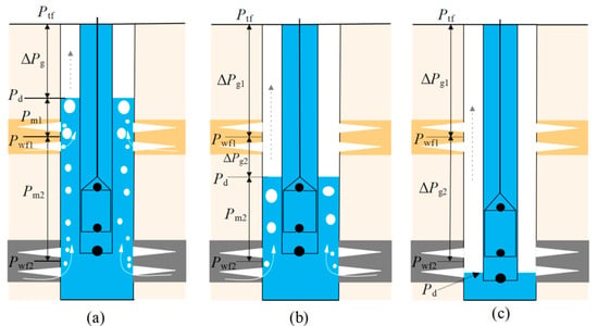
Figure 2.
Pressure distribution in a two-layer coproduction CSG well with different depth of fluid level. (a) The dynamic fluid level is between layer 1 and the ground. (b) The dynamic fluid level is between layer 1 and layer 2. (c) The dynamic fluid level is below layer 2.
From Equation (6), the depth change of the dynamic fluid surface can change the pressure difference between the two layers, while the change in the wellhead pressure could result in the pressure change of layer 1, which could affect the pressure of layer 2. Therefore, a proper wellhead pressure and dynamic fluid surface position can effectively coordinate the production pressure of both layers and suppress interlayer interference.
2.2. Calculation for Pressure Distribution in the Wellbore
Detailed calculations of the wellbore pressure distribution are required to obtain the appropriate wellhead pressure and dynamic fluid surface depth. Based on the fluid flow in the two-layer coproduction well, as shown in Figure 1, the following assumptions are made: the wellbore is perpendicular to the surface; the gas in the oil jacket annulus flows steadily; the mass of the fluid at any annulus section is conserved; and the work and heat exchange is constant [44]. The energy equation for fluid flow in the annulus is
where: p is the pressure, Pa; ρ is the fluid density, kg/m3; h is the wellbore length, m; v is the fluid flow velocity, m/s; f is the friction coefficient; and d is the pipe diameter, m.
Taking the dynamic liquid surface as the boundary, the calculation of wellbore pressure distribution was divided into single-phase gas flow and gas-liquid two-phase flow.
2.2.1. Single-Phase Gas Flow
The following assumptions are made in calculating the differential pressure in the flowing gas section: there is no input and output of work in this process (dW = 0) [44]; the kinetic energy loss in the gas flow is neglected (vdv = 0) [45]. Based on these assumptions, Equation (7) can be simplified as
The equation of the state of the gas is associated with Equation (8), and the following equation is derived after integrating the separated variables.
where: Z is the gas deviation factor, which can be calculated by the Standing-Katz [46] or Dranchuk-Abu-Kassem [47] model; di is the casing ID, mm; do is the tubing OD, mm; and qsc is the daily gas production of the coproduction well, m3.
The wellbore length for which the differential pressure needs to be solved was divided into three sections. The Cullender–Smith method was used to solve Equation (9) [48].
By associating Equation (9) with Equation (10), Equation (11) can be derived.
The pressure value at the specified depth can be calculated using the iterative method.
2.2.2. Gas–Liquid Two-Phase Flow
As shown in Figure 2b, there is a mixed gas-water flow below the dynamic liquid surface of the combined production wells. After the gas enters the wellbore, gas flows through a static liquid. Neglecting the kinetic energy loss of the gas and the frictional energy loss of the gas and the liquid and the pipe wall, the expression for the pressure drop in this section can be expressed as
where: is the density of the gas–liquid (water) mixture kg/m3; and are the starting and ending calculated well depths, m, respectively.
Supposing is the gas void fraction in the water, Equation (12) can be expressed as:
or
where: is the density of the output water, kg/m3; is the density of the output gas, kg/m3; and is the depth of the calculated section of the well, m.
The void fraction can be calculated using the Hasan and Kabir model in two flow regimes: bubble flow and slug flow [33].
Bubble flow:
Slug flow:
The expression for of the transition from bubble to slug flow is
The two-phase section is divided into several sections, and the pressure difference for each section can be calculated. The coefficients in Equations (15)–(17) were determined based on multiple sets of experiments [49,50].
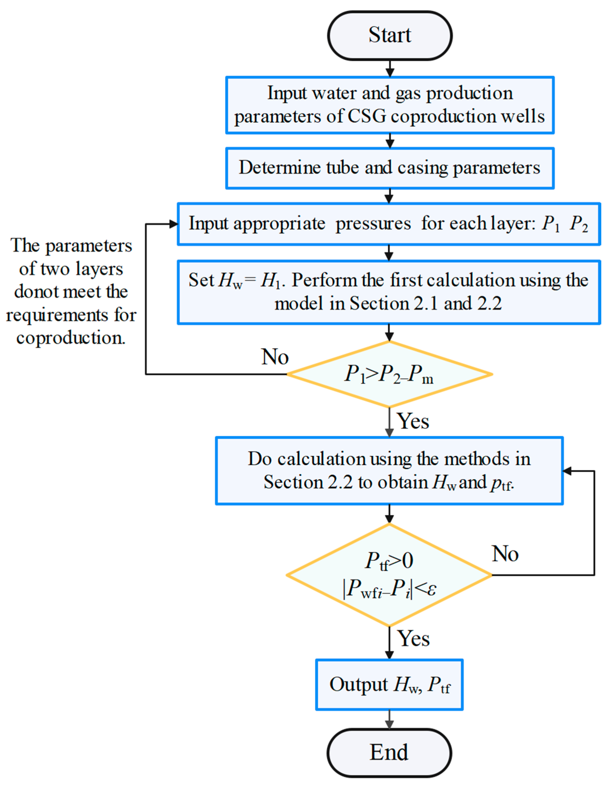
The key parameters (Ptf, Hw) of the coproduction can be obtained by calculation, as shown in Figure 3.
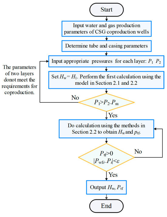
Figure 3.
Calculation flow chart for parameters of CSG coproduction.
3. Experiments
3.1. Device and Method of Experiment
The multilayer physical test device was designed independently and assembled by Jiangsu Tuochuang Scientific Instruments Co. This experimental device can conduct simulations for three layers of CSG coproduction.
The device includes six parts: a gas supply system, a gas flow monitoring system, a pressure monitoring and regulation system, a wellbore simulation unit, and a production layer simulation unit. The gas supply system includes a high-pressure storage tank, an air compressor, a booster system, and a nitrogen tank. The nitrogen tank is a gas resource with a maximum pressure of 12 MPa. The compressed gas is stored in a high-pressure tank with a maximum pressure of 30 MPa. The gas flow monitoring system includes flow meters 17–18. Flow meters 17–18 record the forward gas flow in the upper and lower layer. The pressure monitoring module includes pressure gauges 1–5, with pressure sensors 6–11. The pressure regulation module includes back pressure regulating valves 12–16. Back pressure regulating valves 12–14 are located at the inlet of each of the three core holders and are used to regulate the inlet pressure. The back pressure regulating valve is located at the outlet of the tube and the annulus to regulate the outlet pressure. Pressure sensors 6–11 are located at the front and back of the three core holders to monitor the pressure at the cores. The production layer simulation unit contains three core holders, which can hold φ38 × 200 mm cores. The wellbore simulation unit consists of tubing and casing. The three branches are connected to the casing at different heights, as shown in Figure 4.
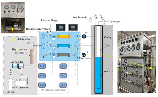
Figure 4.
Schematic diagram of the physical experiment device.
As shown in Figure 4, 1–3 are gate valves; 4, 5 are pressure gauges 6–11 are pressure sensors 12–16 are adjustable backpressure valves. 17, 18 are flow sensors. In this device, the rock cores in the holders represent the production layers with different depths. The inlet pressure controlled by back pressure regulating valves 12–14 represents the reservoir pressure, and the pressure monitored by pressure sensors 7, 9 and 11 represents the bottom hole pressure for each layer. The forward gas flow in flowmeters 17–18 represents the flow from the upper and lower layers. The pressures monitored by pressure gauges 5 and 6 represent the casing and tubing pressure at the ground level, respectively. Different volumes of water were injected into the wellbore, which was used to simulate different heights of dynamic fluid levels.
The steps of the experiment were as follows. 1. Prepare the experimental materials and check the sealing performance of the device. 2. Select suitable cores and install the required cores. 3. Conduct the test according to the set parameters and check the sealing performance of the device again. 4. Open the inlet valve of the device and set the inlet pressure of each layer and the outlet pressure of the wellbore according to the set parameters. 5. After the airflow enters a stable state, record the flow data of each layer and the pressure data of each part of the device. 6. After completing all the experiments, analyze the data from different schemes.
3.2. Materials for Experiments and Processing
These experiments use nitrogen instead of methane for the following reasons. First, methane is flammable, explosive, and toxic. Second, methane is close to the molecular diameter of nitrogen. Moreover, the characteristics of nitrogen and methane gas are close in the CSG adsorption and desorption experiments. Since cores with the same properties are extremely difficult to obtain, pulverized coal (20–30 meshes) of different quality was used instead of cores in this experiment, which may make some characters different from the original layer. In addition, the tubing and casing length of the installation is 1.5 m, which is different from the gas well depth (usually more than 500 m). Due to the limitation of size and pressure sensor precision, the device cannot perform experiments of dynamic liquid level with considerable variations.
To investigate the difference between two-layer coproduction and single-layer production and the effect of pressure changes in layer 1 or 2 on coproduction, fifteen sets of experiments were conducted using the device introduced in Section 3.1. The parameters for each group are shown in Table 1.

Table 1.
Pressure parameters for different experiments.
4. Results and Discussion
According to the analysis above, the pressure distribution in the wellbore is the key to the CSG coproduction. Under the condition that the dimensions of the wellbore structure are determined, it can be concluded through the analysis of Equations (7) and (8) that the factors that have an influence on the pressure gradient in the wellbore are the fluid density in the wellbore and the velocity of the fluids. As for the CSG coproduction process, the specific parameters that have influence on the fluid density and velocity in the wellbore are the wellhead pressure, the gas output of each layer, and the depth of the dynamic fluid level. For different parameters, a combination of theoretical calculation and experimental method is used to analyze the influence of different parameters on the pressure distribution of the wellbore.
4.1. Pressure at the Wellhead
As the production of CSG production layer is very sensitive to pressure change, wellhead pressure is very important for the production of the CSG combined production well of annular gas production. The effects of wellhead pressure on the pressure distribution and production effect in CSG coproduction wellbore were analyzed by theoretical calculation and experiment.
Based on the calculation model in Section 2.2, the pressure distribution calculation of CSG coproduction well under different wellhead pressure conditions was completed, and the results are shown in Figure 5. Relevant parameters for calculation are set as follows: the gas production of upper and lower layers is set as 0.5 × 10⁴ m3/d. The casing size is 5.5 inches and tubing size is 2.875 inches.
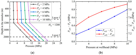
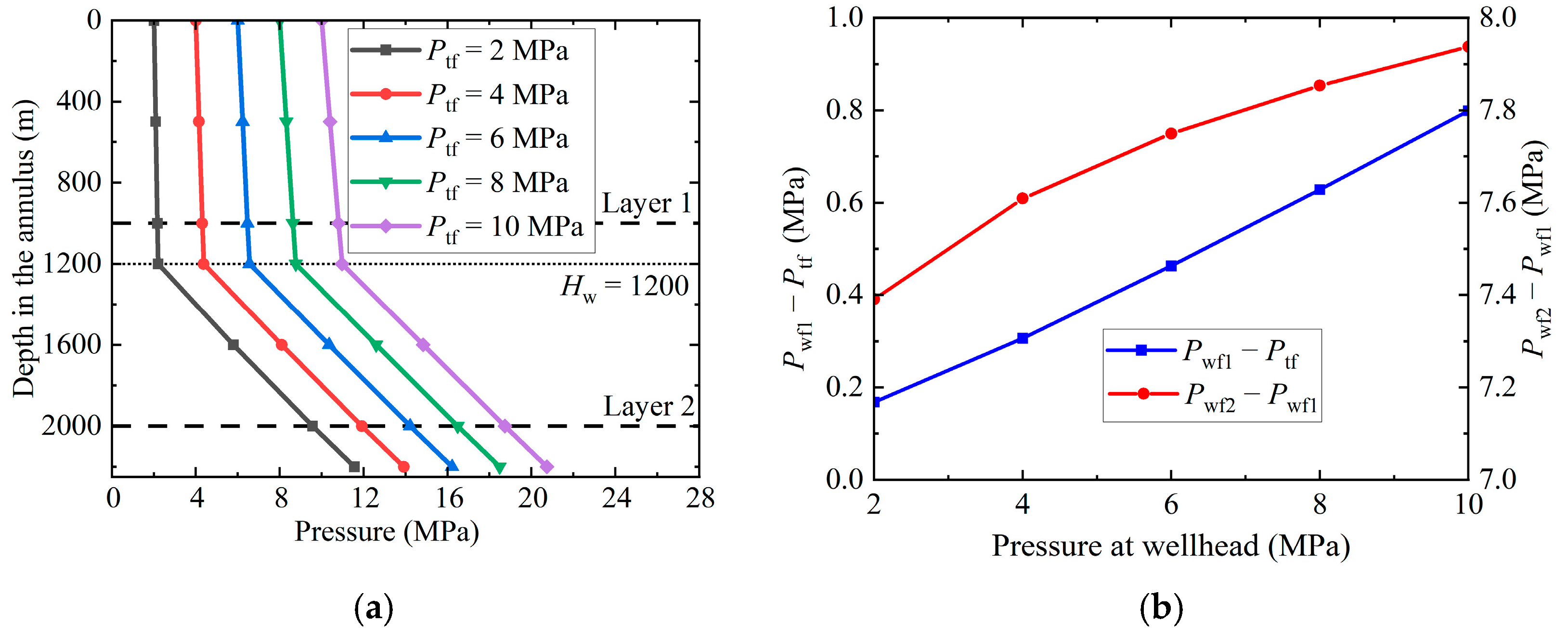
Figure 5.
Pressure distribution of the wellbore of the CSG coproduction well. (a) With different wellhead pressures. (b) Pressure differences of the CSG coproduction well with different Ptf.
As shown in Figure 5a, the variation in wellhead pressure directly affected the production pressure of the two layers when other parameters were constant. The production pressure increased with the increase in wellhead pressure difference at the depth of both layers. As the dynamic liquid surface is located between layer 1 and layer 2 (Hw = 1200 m), at this time there is a gas–liquid mixed two-phase flow between the two layers, as shown in Figure 2b. Therefore, the change in pressure difference between the two layers is less than that between layer 1 and the wellhead. At the same time, the magnitude of pressure difference between layer 1 and wellhead shows an accelerating trend with the increase in wellhead pressure. While the change of pressure difference between the two layers shows a gradual deceleration trend, as shown in Figure 5b. And this may cause a change in the output gas velocity in both layers.
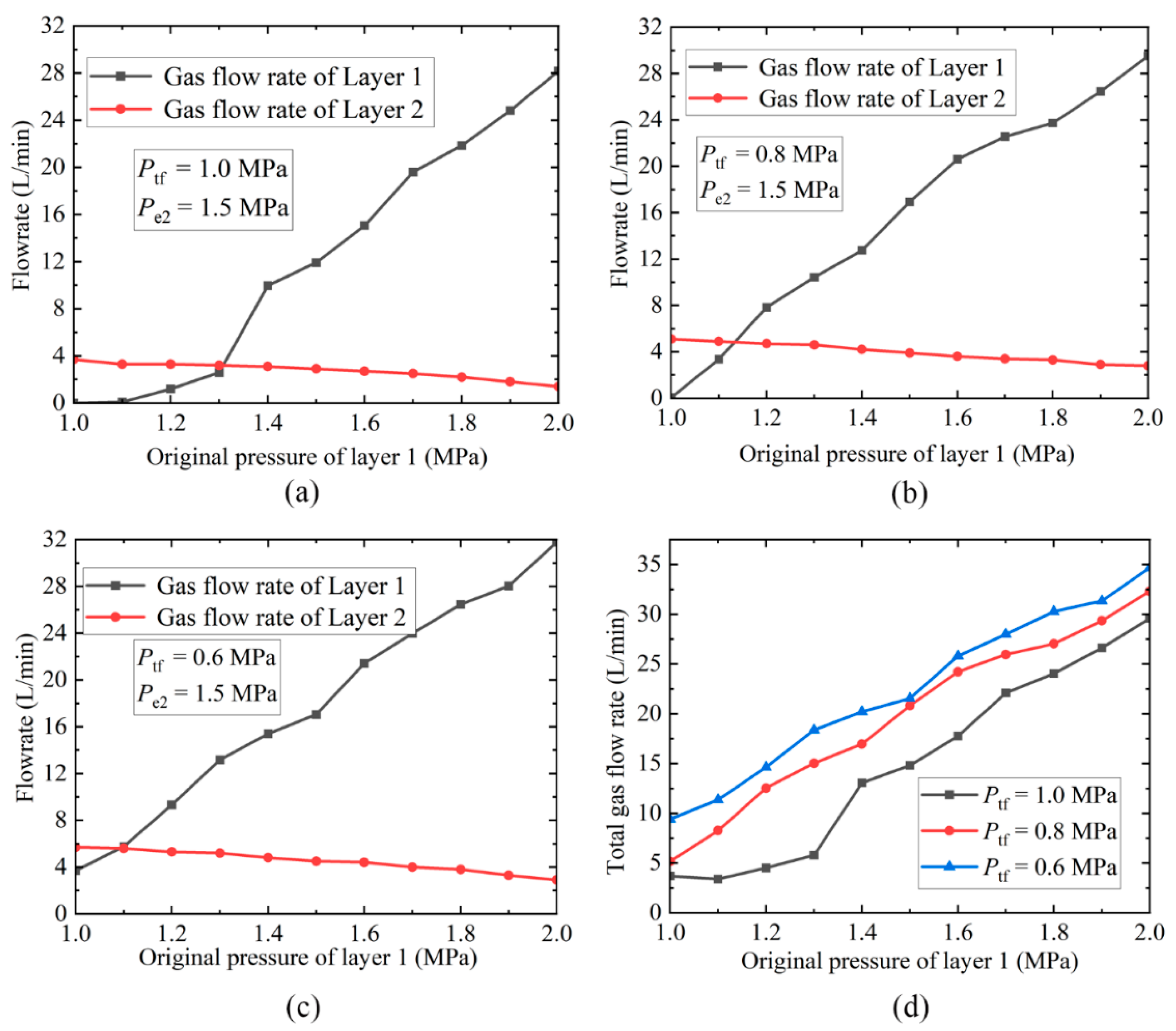
Nine sets of experiments were carried out for coproduction and independent gas production in each layer, with the parameters and materials of the experimental setup kept unchanged. With different Ptf, the total gas flow rate from coproduction increased with increasing Pe1, as shown in Figure 6a–c. The total gas production from coproduction increases with decreasing Ptf. This is consistent with Equations (1)–(3), thus verifying the validity of the experiments. As shown in Figure 6, with the increase in Ptf, the gas flow rate of both layers showed a downward trend, while the gas production of layer 1 rose significantly faster than that of layer 2, which was due to the difference in the geological properties of the cores used for the two layers.
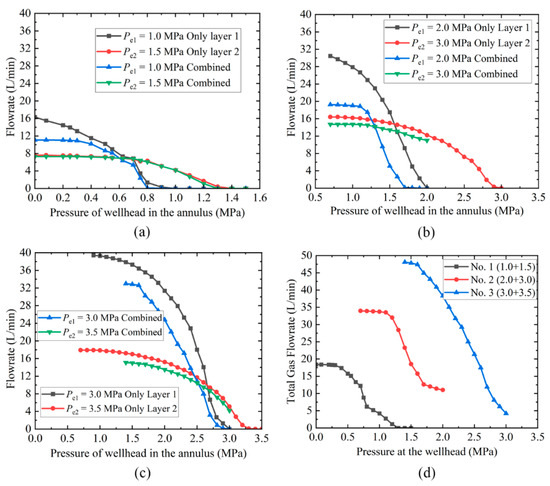
Figure 6.
Gas coproduction rate and independent production of two layers (a) Nos. 1, 10, 11; (b) Nos. 2, 12, 13; (c) Nos. 3, 14, 15; (d) Nos. 1, 2, 3.
The gas production rates of each layer independently are more than that of the individual layer produced in coproduction. This is due to the accumulation of gas produced from the other layer in the wellbore during coproduction, causing an increase in the pressure in the wellbore, which in turn suppresses the gas production rate of the two layers in coproduction. At the same time, the gas flow rate of layer 1 increases significantly faster than that of layer 2, as Ptf decreases during coproduction, which is consistent with the calculation results. In other words, while other conditions are constant, the production flow pressure of layer 1 is affected more relative to layer 2 as Ptf decreases, as shown in Figure 5a.
As shown in Figure 6d, the gas production rate of coproduction continues to increase with decreasing wellhead pressure when the wellhead pressure drops below a critical gas production pressure of the coproduction layer, but the gas production rate of coproduction will tend to stabilize after the wellhead pressure drops to less than 50% of the original layer pressure of the low-pressure layer. In field production, the wellhead pressure can be reduced moderately to increase the gas production of the coproduction wells, but it may not be possible to further increase the total gas production rate of the coproduction wells by producing at very low wellhead pressure.
4.2. Output of Layer 1
To investigate the influence of the output of layer 1 on the wellbore annulus pressure distribution and the effect of combined production, two cases of layer 1 fixed pressure production and fixed output production were analyzed respectively. The fixed output production mode was analyzed in a theoretical method, and the results are shown in Figure 7. The fixed pressure production mode was analyzed by experiment, with the results shown in Figure 8.
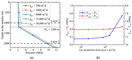
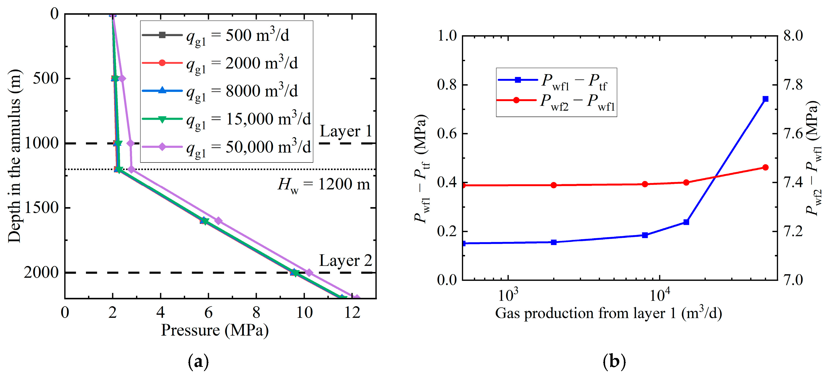
Figure 7.
Pressure distribution of the wellbore of the CSG coproduction well. (a) With different gas production of layer 1; (b) pressure differences of the CSG coproduction well with different qg1.
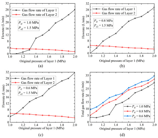
Figure 8.
Coproduction experiments when the original pressure of layer 1 varies. (a) Nos. 1, 10, 11; (b) Nos. 2, 12, 13; (c) Nos. 3, 14, 15; (d) Nos. 1, 2, 3.
As shown in Figure 7, the gas production of layer 1 had little effect on the pressure distribution in the annulus with the variation of gas production in the upper layer. When the gas production of layer 1 grows from 500 m3/d to 50,000 m3/d, the pressure difference between Ptf and Pwf1 increases from 0.15 MPa to 0.74 MPa. The increase in Pwf1 − Ptf is 0.59 MPa, an increase of 393.3% relative to the initial pressure difference. At the same time, Pwf2 − Pwf1 increases from 7.39 MPa to 7.46 MPa. Pwf2 − Pwf1 changes by 0.07 MPa with a variation range of less than 1%. The increase in gas production in layer 1 significantly affects the pressure difference between the wellhead and layer 1. As the gas production of layer 1 changes within 10,000 m3/d, the pressure difference between the two layers’ changes less than 0.03 MPa. The effect on the difference in production pressure between the two layers is slight.
As shown in Figure 8a–c, as Ptf decreases from 1.0 MPa to 0.6 MPa, the minimum and maximum gas production of layer 1 increases from 0.0 L/min and 28.2 L/min to 3.7 L/min and 31.8 L/min, respectively, while the minimum and maximum gas production of layer 2 changes from 1.4 L/min and 3.7 L/min to 2.9 L/min and 5.7 L/min, respectively. When the pressure of layer 1 increases, the gas production rate of layer 1 increases, while the gas production rate of layer 2 gradually decreases. The reason is that when the pressure of layer 1 increases, the production pressure difference of layer 1 gradually increases due to the constant Ptf, and the gas production rate of layer 1 increases, which is consistent with Equations (4)–(6). As the production pressure of layer 1 increases, it will cause the production pressure at layer 2 to increase, which makes the production pressure difference of layer 2 decrease, and this would suppress the gas production rate of layer 2. As shown in Figure 8d, when the production pressure of layer 1 increases, the total gas production rate of coproduction increases with decreasing Ptf. When Ptf, decreases from 1.0 MPa to 0.8 MPa, the gas production rate changes more relative to the decrease in Ptf, from 0.8 MPa to 0.6 MPa. This is consistent with the results in Figure 6d. This further verifies that when Ptf, decreases, the total gas production of coproduction will increase rapidly and then slowly with the continuous decrease in wellhead pressure.
4.3. Output of Layer 2
The gas production and production pressure of layer 2 were analyzed using the same methodology as for layer 1.
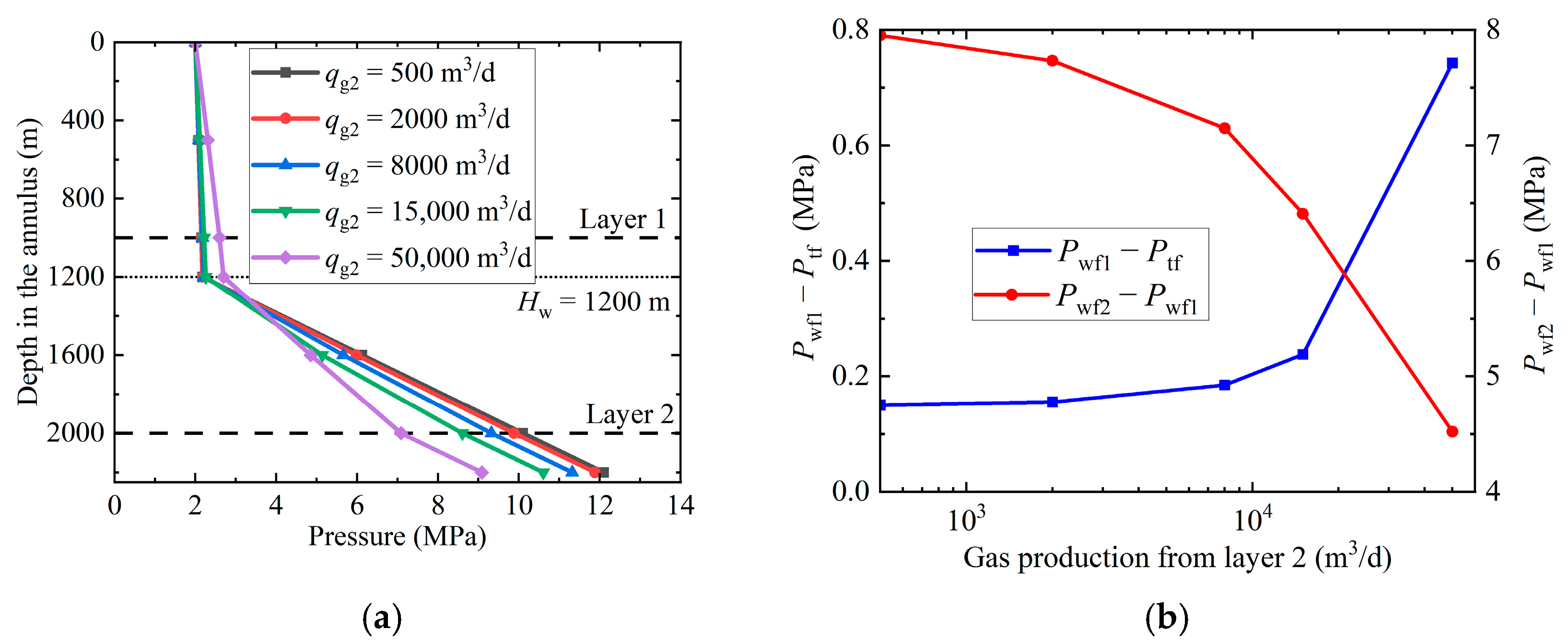
As shown in Figure 9a, under the condition that only the gas production of layer 2 varied, the production pressure of layer 1 changed slightly. This is due to the single-phase gas flow in the portion above the depth of layer 1, where the changes in gas production from layer 2 have a small effect on the pressure gradient. However, the production pressure at the depth of layer 2 is greatly varied. The reason for this is the change in the flow regime in the gas–water mixing section between the two layers due to the change in the amount of gas produced from layer 2. As shown in Figure 9b, when qg2 increased from 500 m3/d to 15,000 m3/d, the pressure difference between Ptf and Pwf1 increases from 0.15 MPa to 0.23 MPa. The increase in Pwf1 − Ptf is 0.08 MPa, an increase of 53.3% relative to the initial pressure difference. At the same time, Pwf2 − Pwf1 decreases from 7.95 MPa to 6.41 MPa. Pwf2 changes by 1.54 MPa with a variation range of 19.4%. While the gas production of layer 2 is 50,000 m3/d, the pressure difference between layer 1 and the wellhead is 0.74 MPa, while the pressure difference between the two layers is 3.43 MPa. These pressure differentials show a large change compared with that of 15,000 m3/d. This is attributed to the change in the flow regime of the gas–water two-phase flow below the dynamic liquid level between the two layers when the gas production grows from 15,000 m3/d to 50,000 m3/d.

Figure 9.
Pressure distribution of the wellbore of the CSG coproduction well. (a) With different gas production of layer 2. (b) Pressure differences of the CSG coproduction well with different qg2.
The results of the experiments related to the impact of the change in output in layer 2 are shown in Figure 10.
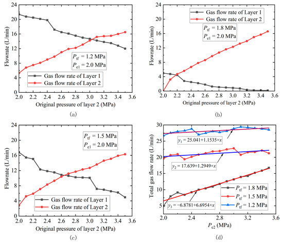
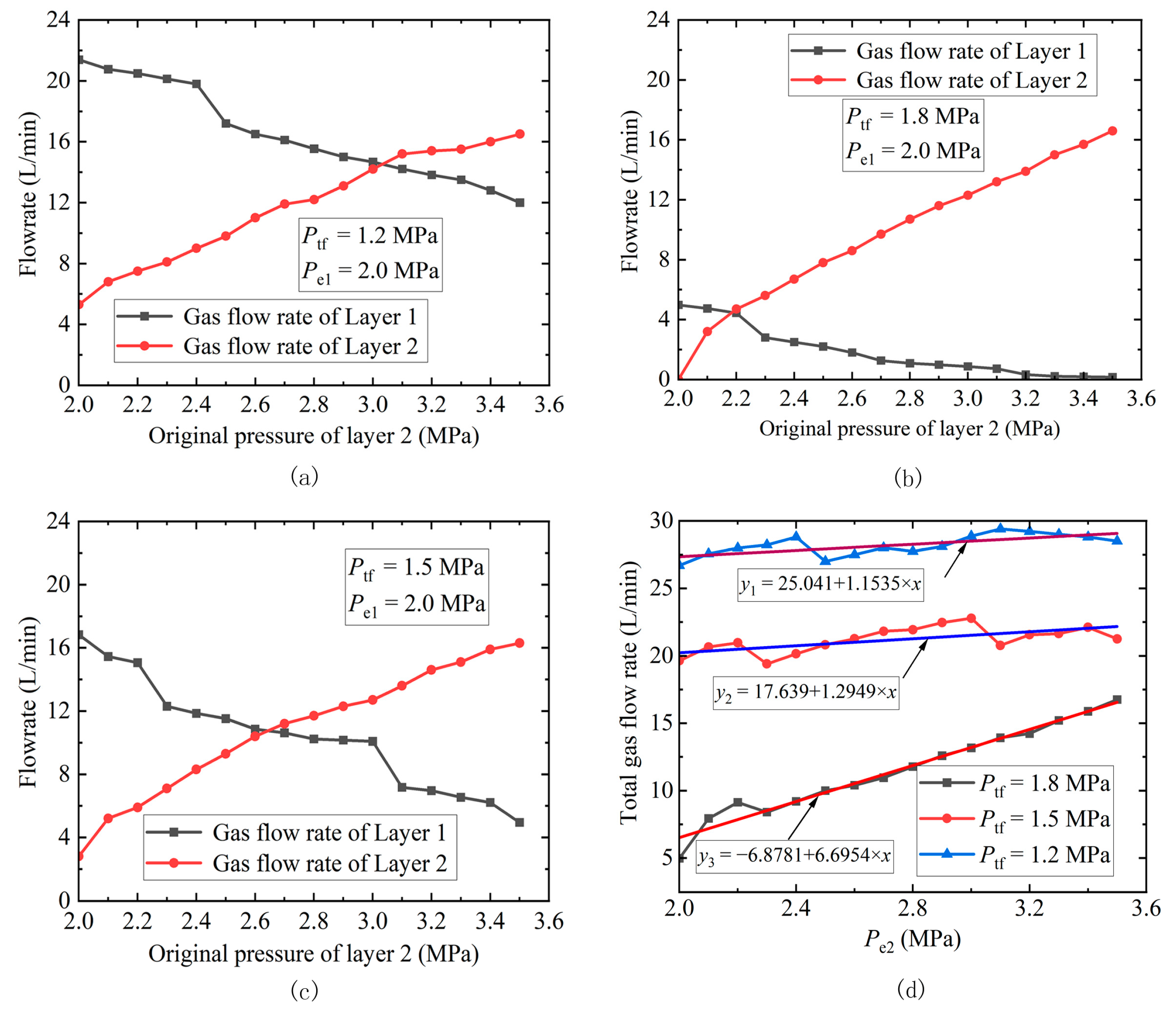
Figure 10.
Flow rate of coproduction experiments when the original pressure of layer 2 varies. (a) Nos. 1, 10, 11; (b) Nos. 2, 12, 13; (c) Nos. 3, 14, 15; (d) Nos. 1, 2, 3.
As shown in Figure 10a–c, as the production pressure of layer 2 gradually increases, the gas flow rate of layer 1 gradually decreases. As the wellhead pressure is 1.2 MPa, the flow rate decreases from 21.39 L/min to 12 L/min. while the gas flow rate of layer 2 increases from 5.3 L/min to 16.5 L/min. This is because the production pressure of layer 2 increases and leads to a gradual increase in pressure in the wellbore, which inhibits the output of layer 1. With the increase in the pressure of layer 2, the production pressure drop of layer 2 increases, which results in the increase in the flow rate of layer 2. As the Ptf increases, the total gas production of the two coproduction layers decreases, as shown in Figure 10d.
With Ptf = 1.8 MPa, the total gas output from the coproduction of the two layers gradually increases with the increase in the production pressure of layer 2. At this time, the wellhead pressure is close to the layer production pressure, and the production capacity of the layers is not effectively released. As the pressure in layer 2 increases, the production capacity of layer 2 is gradually released due to the constant Ptf; thus, the gas production rate of layer 2 continues to increase. The pressure in the wellbore also rises simultaneously, thus inhibiting the gas production of layer 1. The reason for this is that when the wellhead pressure is significantly lower than the production pressure of both layers, when the layer pressure of layer 2 increases, it will not only lead to an increase in the gas production rate of layer 2 but also cause an increase in the wellbore pressure, which will in turn inhibit the decrease in the gas production rate of layer 1. Thus, the overall gas production will not show a noticeable increase.
4.4. Dynamic Fluid Level
The theoretical model was used for the calculation of wellbore pressure in the CSG coproduction wells, and the results are shown in Figure 11.
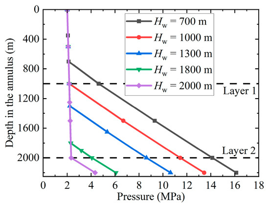
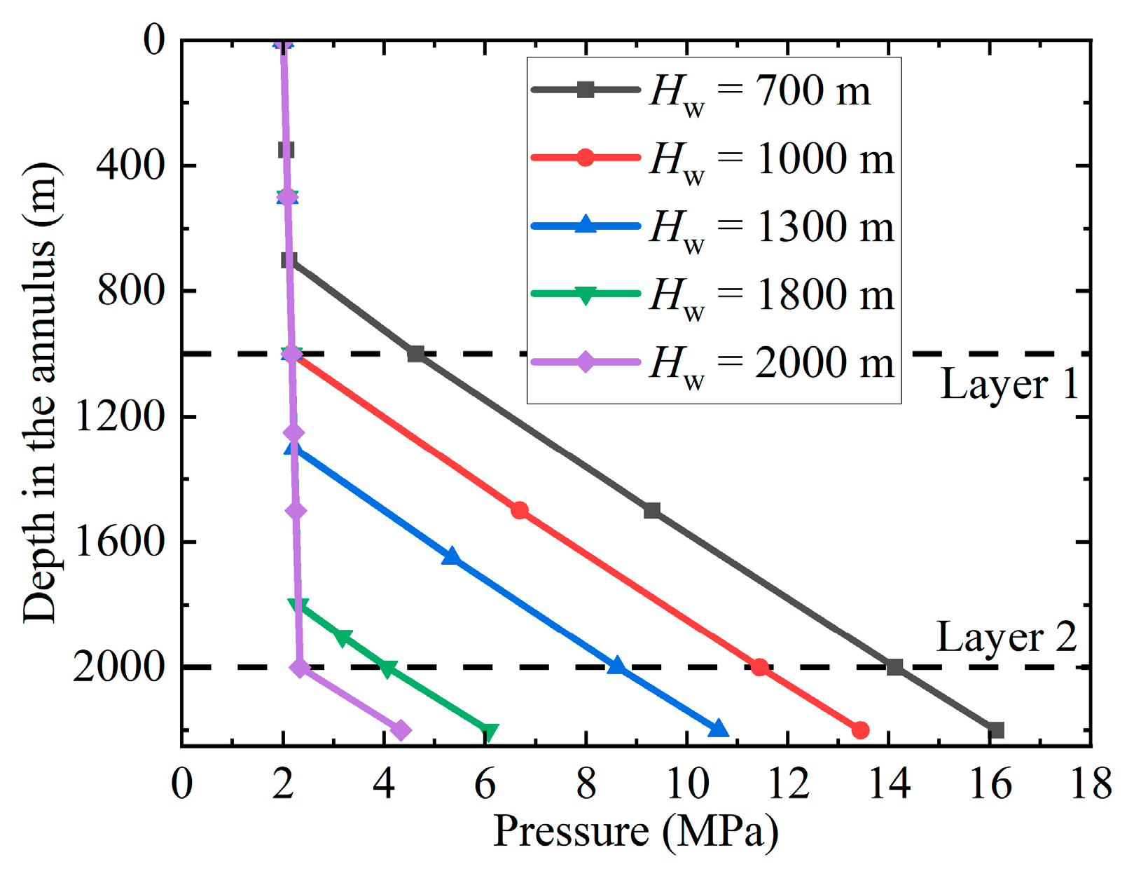
Figure 11.
Pressure distribution of the wellbore of the CSG coproduction well with different depth of dynamic fluid level.
When the depth of the dynamic liquid surface varied, the change in the production pressure of the two layers was significant, as shown in Figure 11. While the dynamic liquid surface was above layer 1, due to the pressure difference between the two phases flow, it would directly increase the production pressure at the depth of layer 1. The magnitude of the increase mainly depended on the value of the depth difference between layer 1 and the dynamic liquid surface. In the case where the dynamic fluid level is between the two layers, the production pressure of layer 1 is mainly affected by the variation in the wellhead pressure of the annular space. However, the production pressure difference between the two layers is affected by the depth variation of the dynamic liquid surface, which means that the production pressure of layer 2 is mainly affected by the depth of the dynamic liquid surface. When the dynamic liquid surface was deeper than layer 2, the dynamic liquid surface mainly affected the pressure distribution below layer 2 in the wellbore annulus. Therefore, the production pressure of the two layers was mainly influenced by the production pressure at the Ptf, Hw and the output pressure of the two layers.
4.5. Pressure Gradient
To facilitate the adjustment of parameters in the field, an analysis of the pressure gradient of the pure gas column and annular gas-liquid two-phase pressure with daily gas production and in-place pressure variation was performed according to the model in Section 3. The range of gas production is 1~50,000 m3/d and the pressure range is 1.0–16.0 MPa. The tubing size in the wellbore is 2.875 inches and the casing size is 5.0 inches. The well depth is set to 2300 m.
The results are shown in Figure 5. The results show that the pressure gradient in the pure gas column section ranges from 6.5 kPa/100 m~0.14 MPa/100 m, while the pressure gradient in the gas-liquid two-phase region ranges from 0.53 to 1.00 MPa/100 m.
As shown in Figure 12a, the pressure drop in the pure gas column section is mainly affected by the pressure, as gas production is below 10,000 m3/d. With an increase in in-situ pressure, the gas density increases, which leads to a linear increase in the pressure drop in the gas column section with gas density. Under the condition of gas production of more than 10,000 m3/d, the increase in frictional resistance in gas flow resulted from an increased gas flow rate. The pressure gradient showed a decreasing and then increasing trend in the range of in situ pressure from 1 to 16.0 MPa. The pressure gradient in the gas column section decreases when the pressure is lower than 4.0 MPa. When the in situ pressure is higher than 4.0 MPa, the gradient change due to frictional resistance gradually decreases as the gas flow velocity gradually slows down due to the pressure increase.
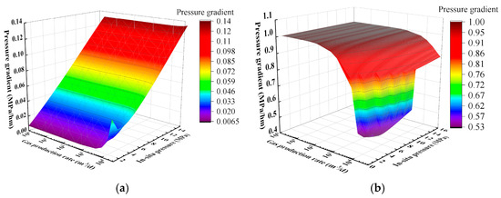
Figure 12.
Pressure gradient influenced by gas production and in situ pressure (a) pure gas section; (b) gas-water two-phase section.
As shown in Figure 12b, when the gas production volume is less than 1000 m3/d, the pressure gradient in the gas-water mixed flow section is mainly influenced by the gravity of both gas and water phases. Moreover, when the gas production volume is greater than 1000 m3/d, the output gas causes the void ratio occupied by the gas in the mixed flow section to increase, which reduces the density of the gas-water mixture in the mixed section. Furthermore, this leads to a rapid decrease in the pressure gradient with the continued growth of gas production. Under this condition, the pressure gradient decreases gradually with an increase in in situ pressure.
The pressure gradient results in the wellbore can effectively guide the adjustment of pressure parameters in the coproduction. This can also provide a basis for determining whether a well should be coproduced through the annulus. Based on the pressure gradient calculation results, the field operator can adjust the wellhead pressure in real time according to the production condition of the coproduction well. Moreover, according to the requirements of the dynamic liquid surface depth, the parameters of the drainage equipment (the stroke and stroke frequency of the pumping unit and the water replenishment flow rate) can be adjusted quickly.
5. Conclusions
It can be obtained from the above analysis that the pressure distribution in the annulus of two-layer CSG coproduction wells is affected by the wellhead pressure, the depth of the dynamic liquid surface, and the gas production rate and gas production pressure of each layer. In order to realize CSG coproduction in the same wellbore annulus, through adjusting the two parameters of wellhead pressure and depth of dynamic liquid surface, a reasonable production pressure difference between the two different pressure system producing layers can be realized, thereby realizing the coproduction of coal system gas. By completing the above study, the following conclusions are concluded:
- (1)
- Based on the wellbore pressure distribution law of CSG coproduction wells, a production parameter control method is established to effectively inhibit interlayer interference in the wellbore. A calculation method for the key parameter control requirements of the coproduction well is established, which provides a basis for the proper parameter regulation of the coproduction wells with an artificial drainage system.
- (2)
- For a given CSG coproduction well, the main factors affecting its wellbore pressure distribution are wellhead pressure, depth of the dynamic fluid surface, and the output of layer 1 and layer 2. Among them, the effect of wellhead pressure on the production pressure of the producing layers is the most obvious, but the effect of wellhead pressure on the interlayer pressure difference is small. An increase in wellhead pressure will directly result in an increase in pressure at both layers’ depths. Also, a decrease in wellhead pressure can lead to a decrease in pressure at both layers’ depths.
- (3)
- Changes in layer 1 output primarily affect the difference between the wellhead pressure and the pressure at the depth of layer 1. It has little effect on the difference between the pressures at the depths of layers 1 and 2. On the other hand, changes in the output of layer 2 affect the production pressure at both layer 1 and layer 2 depths. Therefore, when the dynamic fluid level is located between the two layers, a reasonable dynamic change of the pressure difference between the two layers can be realized by adjusting the depth of the dynamic fluid level. Thus, the interlayer interference in the wellbore can be effectively suppressed.
- (4)
- Fifteen sets of experiments on the effect of production pressure on coproduction were conducted using a set of two-layer coproduction test devices. The experimental results found that the gas production from the coproduction would be lower than the sum of the gas production from the two separate layers. However, by adjusting the wellhead pressure and dynamic fluid level parameters, it is able to make the gas production from the coproduction greater than the single layer production. Moreover, when the wellhead pressure of the combined production is lower than 50% of the low-pressure production layer, the gas production of the coproduction will not increase significantly.
Through theoretical analysis and laboratory experiments, all set results have been completed. The feasibility of suppressing the interlayer interference in the coproduction wellbore of two layers by adjusting the key parameters was verified, which can effectively improve the development benefit of CSG.
Author Contributions
Conceptualization, H.Z. and Y.Q.; methodology, H.Z.; software, H.H.; validation, F.Z. and C.J.; investigation, H.Z.; resources, H.H.; data curation, J.Z.; writing—original draft preparation, H.Z.; writing—review and editing, H.Z.; supervision, F.Z.; project administration, Y.Q.; funding acquisition, F.Z. All authors have read and agreed to the published version of the manuscript.
Funding
This work is supported by National Science and Technology Major Project (2016ZX05066004 & 2017ZX05064004); Major Science and Technology Project of CNOOC Corporation in the 14th Five-Year Plan “Key Technology for Onshore Unconventional Gas Exploration and Development” (ZZGSSAYFWGJS2022454).
Data Availability Statement
The data used to support the findings of this study are included within the article.
Conflicts of Interest
The authors declare no conflict of interest.
References
- Sander, R.; Pan, Z.; Connell, L.D. Laboratory Measurement of Low Permeability Unconventional Gas Reservoir Rocks: A Review of Experimental Methods. J. Nat. Gas Sci. Eng. 2017, 37, 248–279. [Google Scholar] [CrossRef]
- Clarkson, C.R. Production Data Analysis of Unconventional Gas Wells: Review of Theory and Best Practices. Int. J. Coal Geol. 2013, 109–110, 101–146. [Google Scholar] [CrossRef]
- Hamawand, I.; Yusaf, T.; Hamawand, S.G. Coal Seam Gas and Associated Water: A Review Paper. Renew. Sustain. Energy Rev. 2013, 22, 550–560. [Google Scholar] [CrossRef]
- Liu, J.; Sang, S.; Zhou, Z.; Caiqin, B.; Jun, J.; Yansheng, S. Practice and Understanding of Multi-Layer Drainage of CBM Wells in Liupanshui Area. Coal Geol. Explor. 2020, 48, 93–99. [Google Scholar] [CrossRef]
- Zhang, Z.; Qin, Y.; Fu, X.; Yang, Z.; Guo, C. Multi-Layer Superposed Coalbed Methane System in Southern Qinshui Basin, Shanxi Province, China. J. Earth Sci. 2015, 26, 391–398. [Google Scholar] [CrossRef]
- Xu, H.; Tang, D.; Tang, S.; Wenzhong, Z.; Songhang, Z.; Shu, T.; Feng, W. Coal Reservoir Characteristics and Prospective Areas for Jurissic CBM Exploitation in Western Ordos Basin. Coal Geol. Explor. 2010, 38, 26–32. [Google Scholar] [CrossRef]
- Li, G.; Zhang, H. The Geological Model of Coalbed Methane(CBM) Reservoir in the Eastern Ordos Basin. Nat. Gas Geosci. 2015, 26, 160–167. [Google Scholar] [CrossRef]
- Fetisov, V.; Ilyushin, Y.V.; Vasiliev, G.G.; Leonovich, I.A.; Müller, J.; Riazi, M.; Mohammadi, A.H. Development of the Automated Temperature Control System of the Main Gas Pipeline. Sci. Rep. 2023, 13, 3092. [Google Scholar] [CrossRef]
- Meyer, A.G.; Lindenmaier, R.; Heerah, S.; Benedict, K.B.; Kort, E.A.; Peischl, J.; Dubey, M.K. Using Multiscale Ethane/Methane Observations to Attribute Coal Mine Vent Emissions in the San Juan Basin from 2013 to 2021. JGR Atmos. 2022, 127, e2022JD037092. [Google Scholar] [CrossRef]
- Pétron, G.; Miller, B.; Vaughn, B.; Thorley, E.; Kofler, J.; Mielke-Maday, I.; Sherwood, O.; Dlugokencky, E.; Hall, B.; Schwietzke, S.; et al. Investigating Large Methane Enhancements in the U.S. San Juan Basin. Elem. Sci. Anthr. 2020, 8, 038. [Google Scholar] [CrossRef]
- Karacan, C.Ö. Single-Well Production History Matching and Geostatistical Modeling as Proxy to Multi-Well Reservoir Simulation for Evaluating Dynamic Reservoir Properties of Coal Seams. Int. J. Coal Geol. 2021, 241, 103766. [Google Scholar] [CrossRef]
- Karacan, C.Ö. Production History Matching to Determine Reservoir Properties of Important Coal Groups in the Upper Pottsville Formation, Brookwood and Oak Grove Fields, Black Warrior Basin, Alabama. J. Nat. Gas Sci. Eng. 2013, 10, 51–67. [Google Scholar] [CrossRef]
- Adsul, T.; Ghosh, S.; Kumar, S.; Tiwari, B.; Dutta, S.; Varma, A.K. Biogeochemical Controls on Methane Generation: A Review on Indian Coal Resources. Minerals 2023, 13, 695. [Google Scholar] [CrossRef]
- Zhang, J.; Yip, C.; Xia, C.; Liang, Y. Evaluation of Methane Release from Coals from the San Juan Basin and Powder River Basin. Fuel 2019, 244, 388–394. [Google Scholar] [CrossRef]
- Humez, P.; Mayer, B.; Nightingale, M.; Becker, V.; Kingston, A.; Taylor, S.; Bayegnak, G.; Millot, R.; Kloppmann, W. Redox Controls on Methane Formation, Migration and Fate in Shallow Aquifers. Hydrol. Earth Syst. Sci. 2016, 20, 2759–2777. [Google Scholar] [CrossRef]
- Clarkson, C.R.; Behmanesh, H.; Chorney, L. Production-Data and Pressure-Transient Analysis of Horseshoe Canyon Coalbed-Methane Wells, Part II: Accounting for Dynamic Skin. J. Can. Pet. Technol. 2013, 52, 41–53. [Google Scholar] [CrossRef]
- Pearce, J.K.; Hofmann, H.; Baublys, K.; Golding, S.D.; Rodger, I.; Hayes, P. Sources and Concentrations of Methane, Ethane, and CO2 in Deep Aquifers of the Surat Basin, Great Artesian Basin. Int. J. Coal Geol. 2023, 265, 104162. [Google Scholar] [CrossRef]
- Cui, Z.; Su, P.; Liu, L.; Li, M.; Wang, J. Quantitative Characterization, Exploration Zone Classification and Favorable Area Selection of Low-Rank Coal Seam Gas in Surat Block in Surat Basin, Australia. China Pet. Explor. 2022, 35, 108–118. [Google Scholar] [CrossRef]
- Wang, C.; Jia, C.; Peng, X.; Zhu, S.-Y.; Liu, F. A New Well Structure and Methane Recovery Enhancement Method in Two Coal Seams. Energy Sources Part A Recovery Util. Environ. Eff. 2020, 42, 1977–1988. [Google Scholar] [CrossRef]
- Zhang, L.; Shi, J.; Zhang, Q.; Qiao, X.; Xin, C.; Shi, L.; Wang, H. Experimental study on the nuclear magnetic resonance of shale in the southeastern Ordos Basin. J. China Coal Soc. 2018, 43, 2876–2885. [Google Scholar] [CrossRef]
- Zhang, P.; Wang, X.; Zhang, Y.; Wang, C.; Zheng, L.; Gan, M.; Liao, Y. Calculation Model of Bottom Hole Flowing Pressure of Double-Layer Combined Production in Coalbed Methane Wells. Int. J. Energy Res. 2023, 2023, 7506870. [Google Scholar] [CrossRef]
- Meng, S.; Li, Y.; Wang, J.; Gu, G.; Wang, Z.; Xu, X. Co-Production Feasibility ofThree Gases in Coal Measures: Discussion Based on Field Test Well. J. China Coal Soc. 2018, 43, 168–174. [Google Scholar] [CrossRef]
- Guo, C.; Qin, Y.; Sun, X.; Wang, S.; Xia, Y.; Ma, D.; Bian, H.; Shi, Q.; Chen, Y.; Bao, Y.; et al. Physical Simulation and Compatibility Evaluation of Multi-Seam CBM Co-Production: Implications for the Development of Stacked CBM Systems. J. Pet. Sci. Eng. 2021, 204, 108702. [Google Scholar] [CrossRef]
- Wang, Z.; Qin, Y.; Li, T.; Zhang, X. A Numerical Investigation of Gas Flow Behavior in Two-Layered Coal Seams Considering Interlayer Interference and Heterogeneity. Int. J. Min. Sci. Technol. 2021, 31, 699–716. [Google Scholar] [CrossRef]
- Jia, L.; Peng, S.; Xu, J.; Yan, F. Interlayer Interference during Coalbed Methane Coproduction in Multilayer Superimposed Gas-Bearing System by 3D Monitoring of Reservoir Pressure: An Experimental Study. Fuel 2021, 304, 121472. [Google Scholar] [CrossRef]
- Liang, B.; Shi, Y.; Sun, W.; Fang, S.; Jia, L.; Zhao, H. Experiment on influence of inter layer spacing on combined desorption of double-layer coalbed methane reservoir. J. China Univ. Min. Technol. 2020, 49, 54–61+68. [Google Scholar] [CrossRef]
- Wang, Z.; Qin, Y. Physical Experiments of CBM Coproduction: A Case Study in Laochang District, Yunnan Province, China. Fuel 2019, 239, 964–981. [Google Scholar] [CrossRef]
- Jiang, W.; Wu, C.; Wang, Q.; Xiao, Z.; Liu, Y. Interlayer Interference Mechanism of Multi-Seam Drainage in a CBM Well: An Example from Zhucang Syncline. Int. J. Min. Sci. Technol. 2016, 26, 1101–1108. [Google Scholar] [CrossRef]
- Oleg, K.; Andrey, S.; Sergey, S.; Vladimir, I.; Helmut, M. High Productive Longwall Mining of Multiple Gassy Seams: Best Practice and Recommendations. Acta Montan. Slovaca 2022, 27, 152–162. [Google Scholar] [CrossRef]
- Andrey, A.S.; Pavel, N.D.; Vyacheslav, Y.A.; Sergey, A.S. Improvement of Technological Schemes of Mining of Coal Seams Prone to Spontaneous Combustion and Rock Bumps. J. Min. Inst. 2023, 1–13. [Google Scholar]
- Chen, Y.; Luo, J.; Hu, X.; Yang, Y.; Wei, C.; Yan, H. A New Model for Evaluating the Compatibility of Multi-Coal Seams and Its Application for Coalbed Methane Recovery. Fuel 2022, 317, 123464. [Google Scholar] [CrossRef]
- Sadatomi, M.; Sato, Y.; Saruwatari, S. Two-Phase Flow in Vertical Noncircular Channels. Int. J. Multiph. Flow 1982, 8, 641–655. [Google Scholar] [CrossRef]
- Hasan, A.R.; Kabir, C.S. Predicting Multiphase Flow Behavior in a Deviated Well. SPE Prod. Eng. 1988, 3, 474–482. [Google Scholar] [CrossRef]
- Kelessidis, V.C.; Dukler, A.E. Modeling Flow Pattern Transitions for Upward Gas-Liquid Flow in Vertical Concentric and Eccentric Annuli. Int. J. Multiph. Flow 1989, 15, 173–191. [Google Scholar] [CrossRef]
- Papadimitriou, D.A.; Shoham, O. A Mechanistic Model for Predicting Annulus Bottomhole Pressures in Pumping Wells. In Proceedings of the SPE Production Operations Symposium, SPE, Oklahoma City, Oklahoma, 7 April 1991; p. SPE-21669-MS. [Google Scholar]
- Antonio, C.V.M.; Time, R.W. An Experimental and Theoretical Investigation of Upward Two-Phase Flow in Annuli. SPE J. 2002, 7, 325–336. [Google Scholar] [CrossRef]
- An, H.-J.; Langlinais, J.P.; Scott, S.L. Effects of Density and Viscosity in Vertical Zero Net Liquid Flow. J. Energy Resour. Technol. 2000, 122, 49–55. [Google Scholar] [CrossRef]
- Qin, Y.; Moore, T.A.; Shen, J.; Yang, Z.; Shen, Y.; Wang, G. Resources and Geology of Coalbed Methane in China: A Review. Int. Geol. Rev. 2018, 60, 777–812. [Google Scholar] [CrossRef]
- Yang, Z.; Zhang, Z.; Qin, Y.; Wu, C.; Yi, T.; Li, Y.; Tang, J.; Chen, J. Optimization Methods of Production Layer Combination for Coalbed Methane Development in Multi-Coal Seams. Pet. Explor. Dev. 2018, 45, 312–320. [Google Scholar] [CrossRef]
- Ilyushin, Y.V. Development of a Process Control System for the Production of High-Paraffin Oil. Energies 2022, 15, 6462. [Google Scholar] [CrossRef]
- Li, Q.; Xu, J.; Shu, L.; Yan, F.; Pang, B.; Peng, S. Exploration of the Induced Fluid-Disturbance Effect in CBM Co-Production in a Superimposed Pressure System. Energy 2023, 265, 126347. [Google Scholar] [CrossRef]
- Yang, Z.; Li, Y.; Qin, Y.; Sun, H.; Zhang, P.; Zhang, Z.; Wu, C.; Li, C.; Chen, C. Development Unit Division and Favorable Area Evaluation for Joint Mining Coalbed Methane. Pet. Explor. Dev. 2019, 46, 583–593. [Google Scholar] [CrossRef]
- Meng, S.; Li, Y.; Wu, X.; Xu, Y.; Guo, H. Productivity Equation and Influencing Factors of Co-Producing Coalbed Methane and Tight Gas. J. China Coal Soc. 2018, 43, 1709–1715. [Google Scholar] [CrossRef]
- Jin, Z.; Yang, C.; Zhang, S. Gas Production Engineering, 1st ed.; Petroleum Industry Press: Beijing, China, 2004; ISBN 978-7-5021-4902-4. [Google Scholar]
- Liu, X.; Liu, C.; Liu, G. Dynamic Behavior of Coalbed Methane Flow along the Annulus of Single-Phase Production. Int. J. Coal Sci. Technol. 2019, 6, 547–555. [Google Scholar] [CrossRef]
- Standing, M.B.; Katz, D.L. Density of Natural Gases. Trans. AIME 1942, 146, 140–149. [Google Scholar] [CrossRef]
- Dranchuk, P.M.; Abou-Kassem, H. Calculation of Z Factors For Natural Gases Using Equations of State. J. Can. Pet. Technol. 1975, 14, PETSOC-75-03-03. [Google Scholar] [CrossRef]
- Cullender, M.H.; Smith, R.V. Practical Solution of Gas-Flow Equations for Wells and Pipelines with Large Temperature Gradients. Trans. AIME 1956, 207, 281–287. [Google Scholar] [CrossRef]
- Hasan, A.R.; Kabir, C.S.; Rahman, R. Predicting Liquid Gradient in a Pumping-Well Annulus. SPE Prod. Eng. 1988, 3, 113–120. [Google Scholar] [CrossRef]
- Sun, B. Multiphase Flow in Oil and Gas Engineering, 1st ed.; China University of Petroleum Press: Dongying, China, 2013; ISBN 978-7-5636-4225-0. [Google Scholar]


Disclaimer/Publisher’s Note: The statements, opinions and data contained in all publications are solely those of the individual author(s) and contributor(s) and not of MDPI and/or the editor(s). MDPI and/or the editor(s) disclaim responsibility for any injury to people or property resulting from any ideas, methods, instructions or products referred to in the content. |
© 2023 by the authors. Licensee MDPI, Basel, Switzerland. This article is an open access article distributed under the terms and conditions of the Creative Commons Attribution (CC BY) license (https://creativecommons.org/licenses/by/4.0/).