Refined Equivalent Modeling Method for Mixed Wind Farms Based on Small Sample Data

Abstract

For equivalent modeling of mixed wind farms (WFs), existing clustering indicators cannot consider the complex coupling characteristics between different types of wind turbines (WTs). In this paper, a refined equivalent modeling approach based on artificial intelligence technology is proposed. Firstly, the electromechanical transient performance of mixed WFs is analyzed. The WT type, wind speed and direction, and voltage dip are considered the dominant factors affecting the external dynamic response of mixed WFs. Secondly, the equivalent node model is established, including the selection of independent and dependent variables. Then, the multiple artificial neural networks (ANNs) are trained one by one based on small sample data, to fit the nonlinear relationship between the dependent variables and the independent variables. Finally, the dynamic response of the power systems with a mixed WF is simulated in the MATLAB platform. A comparison of the errors in electromechanical phenomena demonstrates that the proposed model can reflect the external characteristics of the test mixed WF in different wind conditions and voltage dips.

1. Introduction

In recent years, large-scale wind farms (WFs) have become popular to reduce the consumption of fossil fuels in China [1,2]. The growing penetration of wind power brings deep changes in the electromechanical transient stability of power systems due to the low inertia and weak voltage support capability of wind power [3,4]. To ensure the safe and stable operation of the changing power systems, grid power operators must conduct extensive simulation analysis in advance; however, large-scale WFs may contain hundreds or even thousands of wind turbines (WTs), which could sharply increase the order of a simulation model and then lead to the “curse of dimensionality” [5]. Therefore, it is significant to develop the WF equivalent models for power system dynamic studies.

Currently, WTs are generally divided into four types, i.e., squirrel-cage induction generator (SCIG), wound rotor induction generator (WRIG), doubly fed induction generator (DFIG), and permanent magnet synchronous generator (PMSG) [6,7]. In the early days, SCIG and WRIG were the mainstream WTs. Due to the lack of power converters, the rotor speeds of these WTs remain almost constant under different wind speeds. In addition, early SCIG- or WRIG-based WFs were not large. The differences in electrical distance and input wind speed between WTs are relatively small, leading to high behavioral correlations among WTs in large disturbance scenarios. Therefore, the single-machine equivalent model, which aggregates all WTs within the WF into one re-scale WT, is recommended for SCIG-based and WRIG-based WFs [8]. However, with the continuous expansion of the WF scale and the emergence of variable-speed constant-frequency WTs, it is difficult to reflect the external characteristics of WFs using the single-machine equivalent model.

For DFIG- or PMSG-based WFs, there are differences in the operating characteristics of WTs within WFs, and the multi-machine equivalent model, which clusters WTs into several groups and aggregates each group into one re-scale WT, generally reflects the dynamic responses of WFs better and has wider applications in practice [9]. Reference [10] provides an overview of equivalent modeling methods for various WFs, as well as the calculation methods for equivalent unit parameters. The key point of the multi-machine equivalent modeling method lies in the selection of clustering indicators and clustering algorithms. On the one hand, the focus of clustering indicators is gradually shifting from mechanical characteristics to electrical characteristics. Wind speed [11,12] and rotor speed [13] are initially chosen as clustering indicators, and later the crowbar action [14,15], chopper action [16], and low-voltage ride through (LVRT) mode [17] receive attention because they can better reflect the differences in dynamic response of WTs. On the other hand, to achieve an optimal number of clusters and higher training speed, some advanced clustering algorithms, such as fuzzy C-means [18], multi-view fuzzy C-means [19], and density-based spatial clustering of applications with noise [20], are applied to the modeling of WFs. With these improved methods, the dynamic characteristics of DFIG- or PMSG-based WFs can be accurately represented.

The dynamic performance of DFIG and PMSG is better but SCIG still exists in the power system because of its low maintenance, complication, and expenses [21,22]. From an economic perspective, WF operators will consider utilizing the complementarity between different types of WTs to build mixed WFs. At present, there is limited literature on equivalent modeling of mixed WFs. For a mixed WF composed of SCIG and DFIG, the WTs are firstly separated based on the WT type, and then a second clustering is performed based on wind speed [5]. In [23], the genetic algorithm is used to solve the equivalence problem of inconsistent parameters between WTs of the same type but this still uses a separate equivalence for SCIG and DFIG. For mixed WFs composed of SCIG and PMSG, references [24,25] also simply separate WTs based on type. It should be pointed out that within mixed WFs, there may be coupling characteristics between different types of WTs. Whether these coupling characteristics have an impact on the external characteristics of mixed WFs, whether the equivalent modeling method based on WT type differences can effectively reflect these coupling characteristics, and how to construct new clustering indicators if the existing ones cannot represent the coupling characteristics, are the issues worth in-depth consideration and research; however, they are not mentioned in the aforementioned literature.

With the progress of artificial intelligence technology, data-driven modeling methods have received increasing attention. At present, the application of artificial intelligence technology in power systems mainly focuses on pattern recognition and prediction [26,27], control and optimization [28,29], and data classification [30]. The success of current artificial intelligence technology is mostly based on a large amount of labeled data. However, there is limited available fault data for dynamic modeling of wind farms. In addition, reference [31] points out that the difficulty of small sample learning is not entirely due to the number of samples. If the data distribution is sparse and loose, and the gap between data sample points is large, even if the number of samples is large it is still difficult to obtain effective information to improve learning performance. In [32], the long short-term memory neural network (LSTM) and support vector machine (SVM) are used separately to fit the entire dynamic response curve of WFs. The results show that the equivalent model based on SVM has significant errors, and LSTM needs more training data. In addition, the LSTM requires longer training time than the BP neural network [33].

Accordingly, this paper proposes an innovative refined equivalent modeling method for mixed WFs. The main contributions are listed as follows:

(1)

The method of using multiple artificial neural networks (ANNs) to identify the electromechanical transient power fluctuation curve of mixed WFs is introduced into the research on equivalent modeling. For small sample data scenarios, the established model has good performance;

(2)

Meaningful insights into how to select the equivalent node model are provided. The WT type, wind speed and direction, and the fault voltage dip are selected as the independent variables of the equivalent node model. The active power and reactive power at the point of connection (POC) are selected as the dependent variables.

The remainder of this paper is organized as follows. In Section 2, the ideas and methods based on artificial intelligence technology are introduced. The external characteristics of mixed WFs are discussed in detail in Section 3. In Section 4, the equivalent node modeling method for mixed WFs is established. The example analysis and conclusions are discussed in Section 5 and Section 6.

2. Ideas and Methods

Different from the coherence-based WF equivalent modeling method, we treat the whole WF as a black box and utilize artificial intelligence technology to explore the mapping relationship between inputs and outputs. The proposed modeling method has the following characteristics:

(1)

It focuses on the input and output characteristics of WFs, without emphasizing the internal topology information and operation principle. The WF structure modeling can be omitted;

(2)

The ANN has a large number of connections, and the weights of the connections correspond to the model parameters. By adjusting these parameters, the ANN can approximate the outputs of nonlinear systems;

(3)

The time spent on modeling is only related to the ANN and its learning algorithm, and no longer depends on the type and number of WTs within one WF.

The difficulty of this equivalent modeling method lies in balancing the accuracy and generalization ability of the equivalent model, as well as obtaining training datasets. Compared to the former, the latter is more challenging. On the one hand, due to the low frequency of short-circuit faults, it is hard to obtain sufficient fault recording data from historical data. On the other hand, due to substantial WTs within one WF, there are massive random combinations of operating conditions between them. In addition, the uncertainty of fault information makes it difficult to meet big data requirements even with simulation data. Therefore, we try to solve the small-sample learning problem.

The wind speed and voltage dip are candidates for the inputs of the black-box model since they are crucial for the dynamic performance of WFs; however, in the electromechanical transient time scale, it is usually considered that the wind speed and direction remain constant, and the voltage dip during the fault period also remains unchanged. Using this set of constants to explore the fluctuation rule of the entire dynamic curve of WFs may produce a large error, especially for small sample data. As a result, a refined equivalent modeling approach is proposed, in which an ANN only predicts the output value at its corresponding time point, and the entire dynamic curve of WFs is obtained by sequentially concatenating the predicted output values at different time points. This method will establish several ANNs to fit the entire dynamic curve of WFs but it is suitable for small sample data. The framework of this method is shown in Figure 1.

3. External Characteristics of Mixed WF

3.1. Composition of Mixed WF

Compared with WFs composed of the same WTs, the concept of mixed WFs includes two meanings. One is the types of WTs in one WF are the same but the parameters between the WTs are different. The other is that the types of WTs in one WF are different. The first one is relatively simple. The differences between the WTs are mainly reflected in the capacity, operation control mode, and control parameters. In this case, the external performance of the mixed WF will not deviate too much from the dynamic response of the WTs contained in it. Therefore, the equivalent WF model can still follow the single-machine model structure. For the second case, the differences between the WTs are directly reflected in the type of power generation technology and the topology. In this case, the mixed WF is the sum of the dynamic response of each type of WT, and its external characteristics may be different from the performance of any type of WT. Therefore, the equivalent WF model can no longer simply follow the single-machine model structure.

Without loss of generality, we carry out an equivalent modeling study on mixed WFs for the second scenario, which integrates the simultaneous existence of three mainstream WTs, i.e., DFIG, PMSG, and SCIG. The parameters of the same type of WTs are identical. The topology of the mixed WF is shown in Figure 2. The model parameters are given in

Table A1. Simulation parameters.

SCIG	Wind turbine
	Blade radius (m)	48	Shaft system stiffness factor (pu/rad)	1.11
	Inertia time constant (s)	3.5	Rated wind speed (m/s)	10
	Cut-in wind speed (m/s)	3	Cut-out wind speed (m/s)	23
	Squirrel-cage induction generator
	Rated power (MW)	2	Rated frequency (Hz)	50
	Rated voltage (kV)	0.69	Stator impedance (pu)	0.01 + j0.1
	Rotor impedance (pu)	0.01 + j0.1	Stator and rotor mutual impedance (pu)	j3
	Grounding transformer
	Rated capacity (MVA)	2	Impedance (pu)	j3
	Rated Ratio (kV)	25/0.575	Rated frequency (Hz)	50
DFIG	Wind Turbine
	Blade radius (m)	31	Shaft system stiffness factor (pu/rad)	1.11
	Inertia time constant (s)	4.32	Rated wind speed (m/s)	12.5
	Cut-in wind speed (m/s)	3	Cut-out wind speed (m/s)	23
	Double-fed induction generators
	Rated power (MW)	1.5	Rated frequency (Hz)	50
	Rated voltage (kV)	0.575	Stator impedance (pu)	0.016 + j0.16
	Rotor impedance (pu)	0.023 + j0.18	Stator and rotor mutual impedance (pu)	j2.9
	Power converters
	Rated capacity of rotor-side converter (MVA)	0.525	Rated capacity of grid-side converter (MVA)	0.75
	DC Bus Rated Voltage (kV)	1.15	DC side bus capacitance (F)	0.01
	Crowbar circuit input threshold (pu)	2	Crowbar circuit cut-out threshold (pu)	0.35
	Crowbar resistance (pu)	0.1
	Grounding transformer
	Rated capacity (MVA)	1.75	Rated frequency (Hz)	50
	Rated Ratio (kV)	25/0.575	Impedance (pu)	0.06
PMSG	Wind turbine
	Blade radius (m)	38	Shaft system stiffness factor (pu/rad)	1.2
	Inertia time constant (s)	4.6	Rated wind speed (m/s)	12.5
	Cut-in wind speed (m/s)	3	Cut-out wind speed (m/s)	23
	Permanent magnet synchronous generator
	Rated power (MW)	2	Rated frequency (Hz)	50
	Rated voltage (kV)	0.69	Rated DC bus voltage (kV)	1.1
	Stator resistance (pu)	0.0001	d-axis inductance of stator (pu)	1.5
	q-axis inductance of stator (pu)	1.5	DC bus capacitor (F)	0.01
	Grounding transformer
	Rated capacity (MVA)	2.5	Rated frequency (Hz)	50
	Rated Ratio (kV)	25/0.69	Impedance (pu)	0.06
Main Transformer	Rated capacity (MVA)	150	Rated frequency (Hz)	50
	Rated Ratio (kV)	220/25	Impedance (pu)	0.135
Cable line	Unit resistance (Ω/km)	0.1153	Unit inductance (Ω/km)	j0.3297

.

3.2. Influencing Factors of External Characteristics of Mixed WF

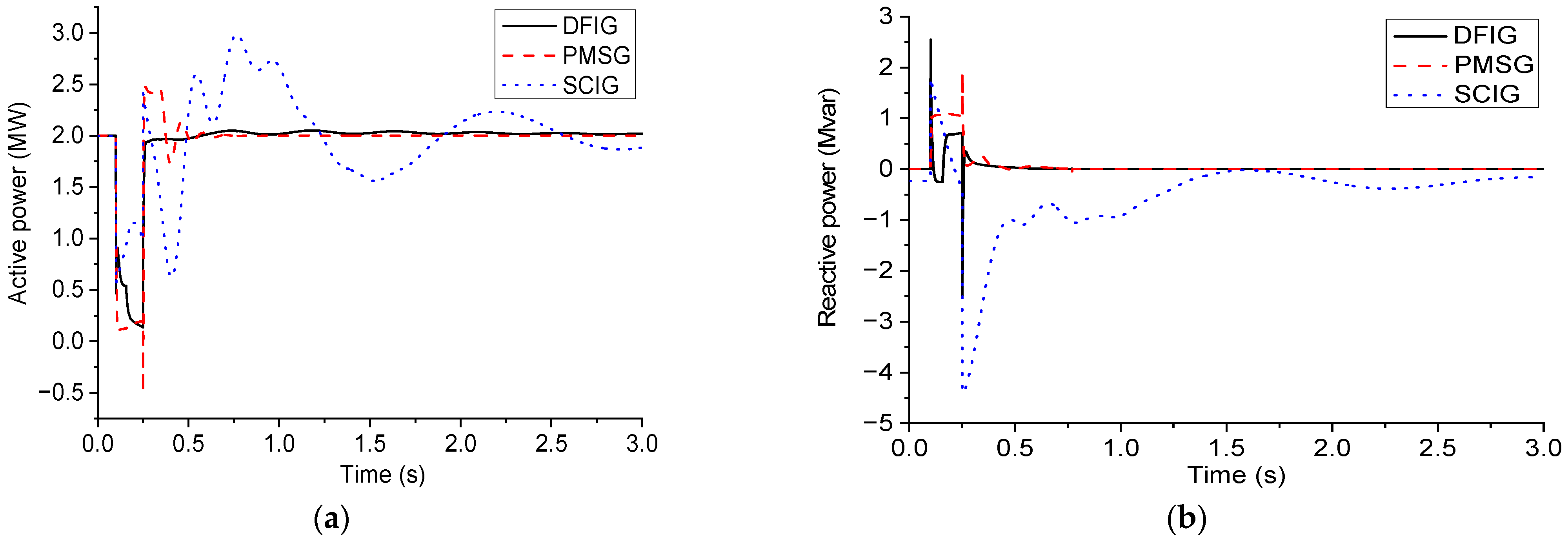
3.2.1. WT Type

As the core device in WFs, WT plays a decisive role in the external characteristics of WFs. In the electromechanical transient process, the dynamic response of the WT mainly depends on its operation control characteristics. Due to the differences in control topology and strategy, different types of WTs have their unique dynamic responses, as shown in Figure 3.

The stator of DFIG is directly connected to the grid, and the rotor is connected to the grid through the power converter. The capacity of the power converter is generally 30% of the capacity of DFIG. To protect the IGBT in the rotor-side converter from electrical and thermal overload, a crowbar circuit is usually added between the rotor and the converter. When the crowbar circuit is activated, the DFIG will lose its power regulation capability, resulting in the WT not only not providing reactive power support to the grid but also needing to absorb part of the reactive power from the grid. After the crowbar circuit is out of service, the DFIG can restore the reactive power support to the grid.

PMSG is connected to the grid through a full-power converter. The increase in the capacity of the power converter makes the power regulation ability and the ability to withstand fault impacts significantly enhanced. Therefore, it is generally only necessary to install a chopper circuit at the DC bus to protect the converter. Compared with DFIG, PMSG can continuously provide reactive power support to the grid during the fault period, and the output reactive power is higher than that of DFIG.

SCIG does not contain a power converter, so its power regulation ability is relatively weak, resulting in relatively intense and lasting active power fluctuations in its dynamic response process. At the same time, it needs to absorb a large amount of reactive power from the grid.

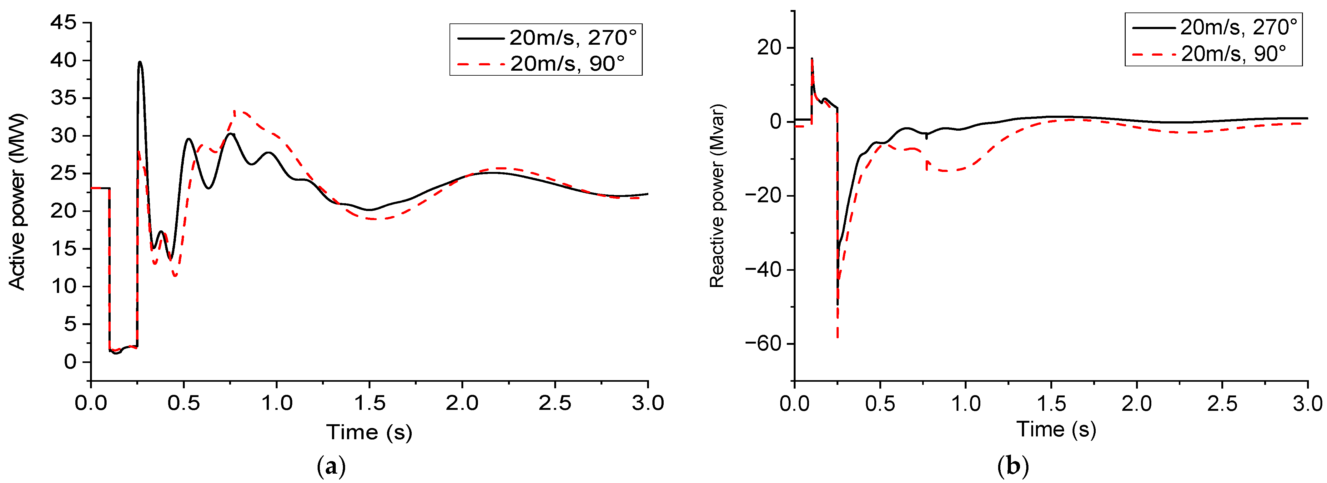
3.2.2. Wind Speed and Direction

In practice, wind power operators will use the wind measurement device to record the wind condition information of WFs, mainly including wind speed and direction. The wind speed reflects the strength of the wind condition, and the wind direction determines the shielding relationship between the upstream and downstream WTs within the WF. Under the wake effect, wind speed and direction jointly determine the operating conditions of WTs and WFs, and the operating conditions of WT and WF before failure will affect their dynamic responses.

It is worth noting that compared with WFs composed of the same WTs, the external characteristics of mixed WFs are more obviously affected by wind conditions due to the difference in WT types. As shown in Figure 4, when the input wind speed is 20 m/s and the wind direction is 270° and 90°, respectively, the distribution of wind resources in the WF has an axisymmetric relationship; however, due to the influence of WT type differences, the external characteristics of the mixed WF show different fluctuation processes.

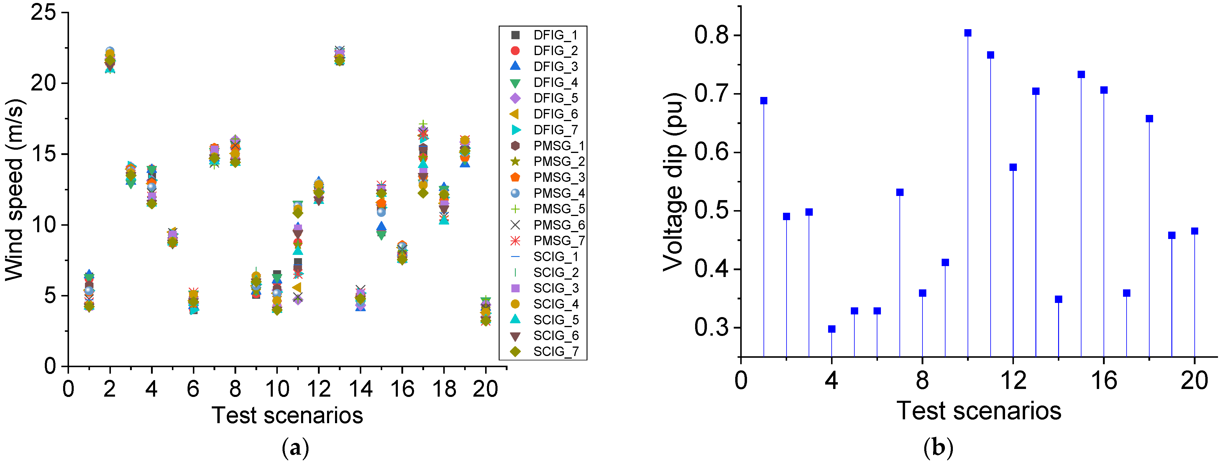
3.2.3. Fault Voltage Dip

As an important fault characteristic quantity, the voltage dip at the POC directly reflects the influence of the grid-side fault on the WF. We know that the voltage dip determines the speed change in the WT, the action of the protection circuit, and the amount of reactive power support provided to the grid, which in turn indirectly affects the external characteristics of the mixed WF, as shown in Figure 5.

3.3. External Characteristic Analysis

In power systems, the fluctuation waveform in time domain simulation is generally in the form of variable period attenuation (divergence), and its characteristic parameters mainly include amplitude, attenuation coefficient, and oscillation period. The external characteristics of mixed WFs are a combination of dynamic response processes of multiple WTs of different types and operating conditions. Although the fluctuation waveforms between WTs are different from each other, the power fluctuation of multiple WTs combined should be smoother than that of a single one due to the smoothing effects. Therefore, for an actual mixed WF, there are regularities in the fluctuation process of its external characteristics. It increases the feasibility of treating the WF as a whole to identify its external characteristics.

4. Equivalent Node Modeling for Mixed Wind Farm

4.1. Equivalent Node Model

In the dynamic equivalent modeling method of power systems, the equivalent model constructed by the coherent theory retains the model structure of the original power device. The advantage is that the existing structure can be directly used for analysis and calculation but the detailed parameters of the system to be equivalent are required in the modeling process. In contrast, the estimation equivalent modeling method directly treats the system as a black box, and the equivalent model is established based on the system identification theory by analyzing the dynamic process of the input and output variables of the system. The equivalent model established using this method is no longer limited to the original model structure of power devices. It provides theoretical support for the equivalent node model of mixed WFs.

The nodes in power systems are described by a set of interrelated variables such as active power, reactive power, voltage amplitude, and phase angle. When the WF is connected to the grid, the change in voltage and frequency at the network node will directly affect the operation state of the WF, that is, the power output from the WF to the network node, which in turn affects the voltage and frequency of the power network. It can be seen that the equivalent node model of the WF should be used to characterize the external power characteristics of the WF. Therefore, the active and reactive power at the POC are selected as the dependent variables of the equivalent node model, i.e., the outputs of the model. According to the analysis in Section 3.2, the external power characteristics of mixed WFs are mainly affected by the WT type, the wind speed and direction, and the fault voltage dip. As a result, these indicators are selected as the independent variables of the equivariant node model, i.e., the inputs of the model.

Considering the expression of WT type information, the wind speed and direction information of the WF is allocated to each WT based on the wake effect, and then we use the input wind speeds of 21 WTs to replace the WT type and the wind speed and direction. Therefore, there are 22 input variables of the equivalent node model of the mixed WF, that is, the input wind speeds of 21 WTs and the fault voltage dip at the POC.

4.2. Experimental Design and Data Collection

The idea of the estimation equivalent modeling method is to extract the intrinsic law of the system by analyzing the sample data, so the selection of the sample must be representative and also pay attention to the balance of the sample category. Based on the principle, the wind direction is evenly divided into 16 azimuths according to the interval. The wind speed is divided into 21 wind speed segments according to the (1 m/s) step size between the cut-in wind speed (3 m/s) and the cut-off wind speed (23 m/s). For the voltage dip, four cases of voltage drop to 0.2 pu, 0.4 pu, 0.6 pu, and 0.8 pu at the POC are considered, with a three-phase short-circuit occurring at 0.1 s, and is removed 0.15 s later. Each combination of wind direction, wind speed, and fault voltage dip constitutes a set of input variables totaling 1344 samples ($16\times 21\times 4=1344$). Furthermore, the wind speed and direction are allocated to each WT based on the wake effect, resulting in 1344 samples of inputs. Actually, there is no specific and rigorous definition for small samples right now, and it is still a topic that needs further exploration and discussion [34,35]. To determine the minimum sample required for an unknown system, a comprehensive judgment should be made from the dimensions of model types, training resources, and accuracy requirements. For the equivalent node model, there are 22 input variables and 1344 samples for training. Based on the ratio of the number of variables to the amount of training samples [36], the dataset with 1344 samples is considered as a small sample condition in this paper.

According to the simulation waveform, during the fault period and the initial stage of fault removal, the external characteristics of the WF fluctuate more violently, and then the fluctuation tends to be stable; therefore, we adopt the variable step size sampling method, that is, in the 0~1 s and 1~3 s periods, the active and reactive power of the WF are collected at intervals of 0.05 s and 0.5 s, respectively.

The sampled data have different physical meanings and different dimensions. To meet the requirements of ANN for training samples, it is necessary to scale the data, that is, the input and output data are limited to [0, 1] or [–1, 1] intervals [37]. In this paper, the linear scale transformation method is used, and the mathematical formula is as follows.

$$x^{\prime }=\frac{x-x_{\min }}{x_{\max }-x_{\min }}$$

(1)

where $x$, $x_{\min }$, $x_{\max }$ are the original value of the training sample, the minimum value, and the maximum value of the training sample, respectively.

4.3. BP-Based Equivalent Modeling

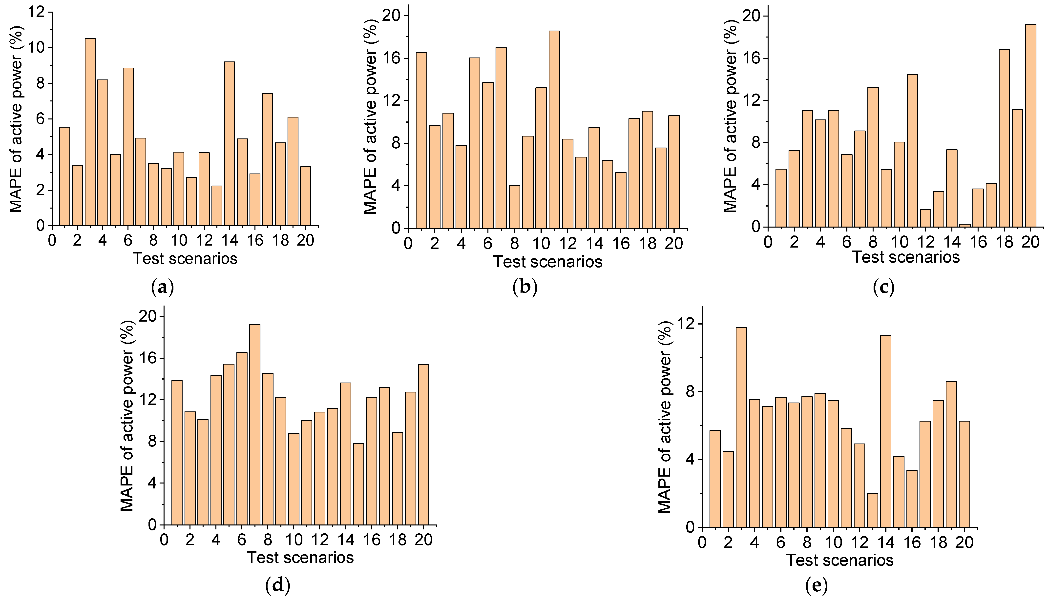
At present, artificial intelligence technology has been widely used in practice. As an important part of ANN, a BP neural network has strong nonlinear mapping ability and parallel information processing capability. In this paper, the back-propagation (BP) neural network is selected to establish the equivalent node model of mixed WFs.

The BP-based equivalent modeling method includes the following contents, i.e., the selection of input and output variables, the determination of the number of implied layers, the number of neurons, and the implementation of the learning algorithm. As mentioned in Section 4.1, the input variables are the wind speeds of 21 WTs and the fault voltage dip at the POC, and the output variables are the active and reactive power of the mixed WF. It is worth noting that the accuracy of the BP neural network can be improved by increasing the number of neurons even if the network structure with a single hidden layer is used. Therefore, we set the number of hidden layers of the neural network to 1, and the number of neurons can be determined using Kolmogorov’s theory [38]. The hyperbolic tangent sigmoid transfer function “tansig” and linear transfer function “purelin” are, respectively, adopted for the hidden layer and output layer. The learning algorithm adopts the error-correction learning algorithm, and the equivalent modeling flow is shown in Figure 6.

5. Example Analysis

The proposed equivalent node modeling method for mixed WFs is implemented in the MATLAB platform, where the number of neurons in the hidden layer is 45 ($2\times 22+1=45$), the learning efficiency is 0.05, and the additional momentum factor is 0.7.

An accurate assessment of the mixed WF equivalent node model requires the construction of appropriate assessment metrics. Considering the numerical characteristics of active and reactive power at the POC, the mean absolute percentage error (MAPE) is used to evaluate the fitting accuracy of the equivalent node model to the active power, and the mean absolute error (MAE) is used to evaluate the fitting accuracy of the equivalent node model to the reactive power. The formulas are shown as follows.

$$E_{\mathrm{MAPE}}=\frac{1}{n}{\displaystyle \sum _{i=1}^n\left|\frac{Y_{fi}(k)-Y_i(k)}{Y_i(k)}\right|}$$

(2)

$$E_{\mathrm{MAE}}=\frac{1}{n}{\displaystyle \sum _{i=1}^n\left|Y_{fi}(k)-Y_i(k)\right|}$$

(3)

where $Y_i(k)$ and $Y_{fi}(k)$ are the electrical quantities of the detailed model and the equivalent model of the WF at the POC, respectively; $n$ is the number of sampling points.

To verify the generalization ability of the established mixed WF equivalent node model, 20 new testing data of wind speed and direction as well as fault voltage dip are generated using simple random sampling. The reason for using simple random sampling is to obtain more balanced testing conditions with fewer testing data. Then, the wind speed of each WT is deduced based on the wake effect, which is shown in Figure 7.

Under the test conditions of Figure 7, the active and reactive power errors of the proposed equivalent node model are calculated according to Equations (2) and (3), respectively. To demonstrate the performance of the proposed model in detail, the differences in accuracy at different stages of the electromechanical transient period, i.e., the pre-fault phase, the early fault phase, the quasi-steady-state phase during the fault, the early fault-recovery phase, and the quasi-steady-state phase during the fault recovery [6,39], are illustrated in Figure 8 and Figure 9. In addition, the average errors during the entire transient process are listed in

Table 1. Model errors (sorted by active power error).

Ranking	$\mathbf{\Delta }\mathit{P}$ (%)	$\mathbf{\Delta }\mathit{Q}$ (Mvar)	Ranking	$\mathbf{\Delta }\mathit{P}$ (%)	$\mathbf{\Delta }\mathit{Q}$ (Mvar)
1	5.78	0.267	11	9.89	0.676
2	6.31	0.383	12	10.05	0.872
3	7.11	0.465	13	10.23	0.765
4	7.50	0.496	14	10.45	0.696
5	7.68	0.561	15	10.86	0.723
6	8.43	0.605	16	11.32	0.705
7	8.60	0.622	17	11.57	0.912
8	9.12	0.593	18	11.68	0.725
9	9.26	0.536	19	12.22	1.160
10	9.53	0.623	20	13.18	1.362

.

As shown in Figure 8 and Figure 9, the active power errors at the early fault phase and early fault recovery phase are relatively large. This is due to the stronger nonlinearity of the dynamic responses during the above time periods. Under the same number of training samples, the fitting performance of BP neural networks is relatively poor compared to the other three time periods. For the overall fitting characteristics of the proposed equivalent node model listed in Table 1, the active and reactive power errors are relatively concentrated, which is mainly because the equilibrium of sample types was considered in the experimental design stage, and the sampled data was subjected to linear scale transformation. Moreover, we adopt the refined equivalent modeling method, in which a BP neural network only predicts the output value at its corresponding time point, instead of directly predicting an entire dynamic curve of the mixed WF. In the proposed method, the error of the whole power curve is jointly determined by all BP neural networks, which in turn reduces the influence of the volatility of the output of a single BP neural network on the error, and ensures that the established equivalent node model of mixed WFs has good stability.

The performance of the equivalent node model at each time point under the ranking first test data, which is the test group with the smallest error, is shown in

Table 2. Output value of the equivalent node model and actual value with the ranking first test data.

Time (s)	Active Power			Reactive Power
	Measured Value (MW)	Output of the Equivalent Node Model (MW)	$\mathbf{\Delta }\mathit{P}$ (%)	Measured Value (Mvar)	Output of the Equivalent Node Model (Mvar)	$\mathbf{\Delta }\mathit{Q}\left(\mathbf{Mvar}\right)$
0.00	12.428	11.821	4.884	1.890	1.866	0.024
0.05	12.428	11.821	4.884	1.890	1.866	0.024
0.10	6.938	6.147	11.401	19.192	19.102	0.089
0.15	8.736	9.353	7.063	20.763	20.971	0.208
0.20	10.073	10.146	0.725	17.947	17.248	0.698
0.25	9.396	9.372	0.255	16.427	16.556	0.129
0.30	17.724	21.361	20.520	−9.978	−10.140	0.162
0.35	13.554	11.903	12.181	−6.177	−5.691	0.486
0.40	8.608	7.638	11.269	−2.853	−2.851	0.002
0.45	10.466	10.095	3.545	−1.594	−1.869	0.275
0.50	14.347	12.836	10.532	−1.269	−1.210	0.059
0.55	14.722	14.509	1.447	−0.415	−0.436	0.021
0.60	12.03	11.551	3.982	0.777	0.670	0.107
0.65	11.45	11.026	3.703	1.200	1.090	0.111
0.70	13.488	12.751	5.464	1.029	0.264	0.764
0.75	14.378	13.611	5.335	1.010	0.961	0.049
0.80	13.165	12.06	8.393	1.417	1.037	0.380
0.85	12.294	12.169	1.017	1.628	0.695	0.933
0.90	12.953	12.392	4.331	1.599	1.090	0.510
0.95	13.541	13.406	0.997	1.525	0.959	0.566
1.00	13.015	12.815	1.537	1.633	0.873	0.760
1.50	12.049	11.287	6.324	1.988	2.075	0.086
2.00	12.749	11.91	6.581	1.831	1.741	0.090
2.50	12.417	11.799	4.977	0.933	1.049	0.116
3.00	12.428	12.022	3.267	1.059	1.083	0.024

. The error at all time points is within an acceptable range, except for the active power error exceeding 20% at 0.3 s. The three-phase short-circuit occurs at 0.1 s, and is removed at 0.25 s. 0.3 s is the first time point after fault recovery. During this stage, the fluctuation of the dynamic curve is more severe, and the corresponding equivalent error is generally large. Under the average action of all BP neural networks, the active power error of the entire curve is 4.884%, which can represent the external characteristics of the mixed WF.

Figure 10 depicts the dynamic responses of the detailed model and the equivalent node model at the POC under the ranking 20th test scenario in Table 1. It can be seen that this error of the equivalent node model is the largest among 20 test scenarios but the dynamic response curve of the proposed model can still match the fluctuation process of the detailed model of the WF in shape and trend. Furthermore, the equivalent node model represents the reactive power curve relatively better compared to the active power curve, which is mainly because the nonlinearity of the reactive power is weaker than the active power during the electromechanical transient process, and, thus, the BP neural network can converge to the globally optimal solution more easily based on the small sample data.

6. Conclusions

From the viewpoint of exploring the nonlinear mapping relationship between the inputs and outputs of mixed WFs, a refined equivalent modeling method based on small sample data is proposed in this paper. This approach uses several BP neural networks to fit the dynamic power responses of the WF, effectively avoiding the phenomenon of significant errors when existing methods only use a single BP neural network to directly generate the entire curve. The equivalent model established using the proposed method has strong applicability. In addition, the inputs and outputs of the equivalent node model are designed based on theoretical analysis and simulation verification. The constructed input variables can take main factors such as WT type, wind speed, wind direction, the wake effect, and fault voltage dip into account.

The simulations were carried out on a personal computer with the following specifications: An 11th Gen Intel(R) Core (TM) i7-1165G7 @ 2.80 GHz, 16 GB of RAM. The average training time was 78 s. For data sampling, the average simulation time for one set of detailed WF was 352 s, and the total simulation time for 1344 sets was approximately 132 h.

The main drawback of this refined equivalent modeling method is that the training algorithm does not have the ability to eliminate measurement errors and the impact of noise since the situation where the training set contains field-measured data has not been considered yet. In future work, advanced small sample learning methods can be combined with filtering methods to further improve the accuracy and engineering utility value of the proposed equivalent node model.

References

1. Global Wind Energy Council. Global Wind Report 2021; Global Wind Energy Council: Brussels, Belgium, 2021; pp. 6–7. [Google Scholar]
2. Wu, J.; Xiao, J.; Hou, J.; Lyu, X. Development potential assessment for wind and photovoltaic power energy resources in the main desert–gobi–wilderness areas of China. Energies 2023, 16, 4559. [Google Scholar] [CrossRef]
3. Agarala, A.; Bhat, S.; Mitra, A.; Zycham, D.; Sowa, P. Transient stability analysis of a multi-machine power system integrated with renewables. Energies 2022, 15, 4824. [Google Scholar] [CrossRef]
4. Skibko, Z.; Hołdynski, G.; Borusiewicz, A. Impact of wind power plant operation on voltage quality parameters—Example from Poland. Energies 2022, 15, 5573. [Google Scholar] [CrossRef]
5. Fernández, L.M.; García, C.A.; Saenz, J.R.; Jurado, F. Equivalent models of wind farms by using aggregated wind turbines and equivalent winds. Energy Convers. Manag. 2009, 50, 691–704. [Google Scholar] [CrossRef]
6. IEC 61400-27-1; Wind Turbines—Part 27-1: Electrical Simulation Models—Wind Turbines. International Electrotechnical Commission: Geneva, Switzerland, 2015.
7. WECC Renewable Energy Modeling Task Force. WECC Wind Power Plant Dynamic Modeling Guidelines; EPRI: Washington, DC, USA, 2014. [Google Scholar]
8. Trudnowski, D.J.; Gentile, A.; Khan, J.M.; Petritz, E.M. Fixed-speed wind-generator and wind-park modeling for transient stability studies. IEEE Trans. Power Syst. 2004, 19, 1911–1917. [Google Scholar] [CrossRef]
9. Chao, P.; Li, W.; Liang, X.; Xu, S.; Shuai, Y. An analytical two-machine equivalent method of DFIG-based wind power plants considering complete FRT processes. IEEE Trans. Power Syst. 2021, 36, 3657–3667. [Google Scholar] [CrossRef]
10. Zou, J.; Peng, C.; Yan, Y.; Zheng, H.; Li, Y. A survey of dynamic equivalent modeling for wind farm. Renew. Sustain. Energy Rev. 2014, 40, 956–963. [Google Scholar] [CrossRef]
11. Akhmotov, V.; Knudsen, H. An aggregate model of a grid-connected, large-scale, offshore wind farm for power stability investigations—Importance of windmill mechanical system. Int. J. Electr. Power Energy Syst. 2002, 24, 709–717. [Google Scholar] [CrossRef]
12. Brochu, J.; Larose, C.; Gagnon, R. Validation of single- and multiple-machine equivalents for modeling wind power plants. IEEE Trans. Energy Convers. 2011, 26, 532–541. [Google Scholar] [CrossRef]
13. Teng, W.; Wang, X.; Meng, Y.; Shi, W. Dynamic clustering equivalent model of wind turbines based on spanning tree. J. Renew. Sustain. Energy 2015, 7, 063126. [Google Scholar] [CrossRef]
14. Zhu, Q.; Ding, M.; Han, P. Equivalent modeling of DFIG-based wind power plant considering crowbar protection. Math. Probl. Eng. 2016, 2016, 8426492. [Google Scholar] [CrossRef]
15. Wu, Z.; Cao, M.; Li, Y. An equivalent modeling method of DFIG-based wind farm considering improved identification of Crowbar status. Proc. CSEE 2022, 42, 603–614. [Google Scholar]
16. Zhu, Q.; Ding, M. Equivalent modeling of PMSG-based wind power plants considering LVRT capabilities: Electromechanical transients in power systems. SpringerPlus 2016, 5, 2037. [Google Scholar]
17. Jin, Y.; Wu, D.; Ju, P.; Rehtanz, C.; Wu, F.; Pan, X. Modeling of wind speeds inside a wind farm with application to wind farm aggregate modeling considering LVRT characteristic. IEEE Trans. Energy Convers. 2020, 35, 508–519. [Google Scholar] [CrossRef]
18. Zou, J.; Peng, C.; Xu, H.; Yan, Y. A Fuzzy clustering algorithm-based dynamic equivalent modeling method for wind farm with DFIG. IEEE Trans. Energy Convers. 2015, 30, 1329–1337. [Google Scholar] [CrossRef]
19. Han, J.; Li, L.; Song, H.; Liu, M.; Song, Z.; Qu, Y. An equivalent model of wind farm based on multivariate multi-scale entropy and multi-view clustering. Energies 2022, 15, 6054. [Google Scholar] [CrossRef]
20. Wang, Y.; Li, Y.; Xie, H.; Wu, B.; Yang, Y. Cluster division in wind farm through ensemble modelling. IET Renew. Power Gener. 2021, 16, 1299–1315. [Google Scholar] [CrossRef]
21. Chandra, D.R.; Kumari, M.S.; Sydulu, M.; Grimaccia, F.; Mussetta, M.; Leva, S.; Duong, M.Q. Impact of SCIG, DFIG wind power plant on IEEE 14 bus system with small signal stability assessment. In Proceedings of the 2014 Eighteenth National Power Systems Conference, Guwahati, India, 18–20 December 2014. [Google Scholar]
22. Nafisa, M.T.; Jahan, E.; Mannan, M.A. Design and analysis of a grid-tied dual rotor PMSG and SCIG-based wind farms. In Proceedings of the 2021 IEEE 9th Region 10 Humanitarian Technology Conference, Bangalore, India, 30 September–2 October 2021. [Google Scholar]
23. Li, H.; Yang, C.; Zhao, B.; Wang, H.S.; Chen, Z. Aggregated models and transient performances of a mixed wind farm with different wind turbine generator systems. Electr. Power Syst. Res. 2012, 92, 1–10. [Google Scholar] [CrossRef]
24. Leon, A.E.; Mauricio, J.M.; Gomez-Exposito, A.; Solsona, J.A. An improved control strategy for hybrid wind farms. IEEE Trans. Sustain. Energy 2010, 1, 131–141. [Google Scholar] [CrossRef]
25. Teninge, A.; Roye, D.; Bacha, S.; Duval, J. Low voltage ride-through capabilities of wind plant combining different turbine technologies. In Proceedings of the 2009 13th European Conference on Power Electronics and Applications, Barcelona, Spain, 8–10 September 2009. [Google Scholar]
26. Lee, S.; Kang, S.; Lee, G.-S. Predictions for Bending Strain at the Tower Bottom of Offshore Wind Turbine Based on the LSTM Model. Energies 2023, 16, 4922. [Google Scholar] [CrossRef]
27. Chen, K.; Hu, J.; He, J. Detection and classification of transmission line faults based on unsupervised feature learning and convolutional sparse autoencoder. IEEE Trans. Smart Grid 2018, 9, 1748–1758. [Google Scholar]
28. Yang, J.; Zheng, S.; Song, D.; Su, M.; Yang, X.; Joo, Y.H. Data-driven modeling for fatigue loads of large-scale wind turbines under active power regulation. Wind. Energy 2021, 24, 558–572. [Google Scholar] [CrossRef]
29. Routray, A.; Reddy, Y.S.; Hur, S.-H. Predictive Control of a Wind Turbine Based on Neural Network-Based Wind Speed Estimation. Sustainability 2023, 15, 9697. [Google Scholar] [CrossRef]
30. Zhang, R.; Yao, W.; Shi, Z.; Ai, X.; Tang, Y.; Wen, J. Encoding time series as images: A robust and transferable framework for power system DIM identification combining rules and VGGNet. IEEE Trans. Power Syst. 2023, 38, 5781–5793. [Google Scholar] [CrossRef]
31. Shen, H. Research on Virtual Sample Generation Technology and Its Application to Industrial Modeling. Master’s Thesis, Beijing University of Chemical Technology, Beijing, China, 2018. [Google Scholar]
32. Chen, S. Study on the equivalent modeling of wind power farm based on LSTM multi-type wind turbine generators. J. Shandong Agric. Univ. 2020, 51, 294–297. [Google Scholar]
33. Ding, X.; Pan, X.; He, D.; Liang, W.; Sun, X.; Guo, J. Wind farm dynamic equivalent modeling by GA-optimized GRU-LSTM-FC combined network. Electr. Power Autom. Equip. 2023, 43, 119–125. [Google Scholar]
34. Saufi, S.R.; Ahmad, Z.A.B.; Leong, M.S.; Lin, M.H. Gearbox fault diagnosis using a deep learning model with limited data sample. IEEE Trans. Ind. Inform. 2020, 16, 6263–6271. [Google Scholar] [CrossRef]
35. Wu, Y.; Liu, L.; Qian, S. A small sample bearing fault diagnosis method based on variational mode decomposition, autocorrelation function, and convolutional neural network. Int. J. Adv. Manuf. Technol. 2023, 124, 3887–3898. [Google Scholar] [CrossRef]
36. Liu, J.; Qu, F.; Hong, X.; Zhang, H. A small-sample wind turbine fault detection method with synthetic fault data using generative adversarial nets. IEEE Trans. Ind. Inform. 2019, 15, 3877–3888. [Google Scholar] [CrossRef]
37. Zou, A.; Yang, C.; Wang, Y. A new method for stability analysis of recurrent neural networks with interval time-varying delay. IEEE Trans. Neural Networ. 2010, 21, 339–344. [Google Scholar]
38. Xu, Z.; Ding, M. Empirical model for capacity credit evaluation of utility-scale PV plant. IEEE Trans. Sustain. Energy 2017, 8, 94–103. [Google Scholar]
39. Zhu, Q.; Tao, J.; Deng, T.; Zhu, M. A general equivalent modeling method for DFIG wind farms based on data-driven modeling. Energies 2022, 15, 7205. [Google Scholar] [CrossRef]
Figure 1. Framework of refined equivalent modeling method.
Energies 16 07191 g001
Figure 2. Mixed WF topology.
Energies 16 07191 g002
Figure 3. Dynamic responses of different types of WTs: (a) Active power; (b) Reactive power.
Energies 16 07191 g003
Figure 4. Characteristics of mixed WF under different wind conditions: (a) Active power; (b) Reactive power.
Energies 16 07191 g004
Figure 5. Characteristics of mixed WF under different voltage dips: (a) Active power; (b) Reactive power.
Energies 16 07191 g005
Figure 6. Flow chart of equivalent modeling for the mixed WF.
Energies 16 07191 g006
Figure 7. Twenty test scenarios: (a) Wind speed scenarios; (b) Voltage dip scenarios.
Energies 16 07191 g007
Figure 8. Active power response error of the proposed models: (a) Pre-fault phase; (b) Early fault phase; (c) Quasi-steady-state phase during the fault; (d) Early fault-recovery phase; (e) Quasi-steady-state phase during the fault recovery.
Energies 16 07191 g008
Figure 9. Reactive power response error of the proposed models: (a) Pre-fault phase; (b) Early fault phase; (c) Quasi-steady-state phase during the fault; (d) Early fault-recovery phase; (e) Quasi-steady-state phase during the fault recovery.
Energies 16 07191 g009
Figure 10. Dynamic power response of the mixed WF at POC: (a) Active power; (b) Reactive power.
Energies 16 07191 g010