Using the Exact Equivalent π-Circuit Model for Representing Three-Phase Transmission Lines Directly in the Time Domain

Abstract

This paper presents a novel three-phase transmission line model for electromagnetic transient simulations that are executed directly within the time domain. This model relies on distributed and frequency-dependent parameters, as well as employs modal transformation for its implementation. The single-phase model of the exact equivalent $\pi$-circuit is utilized for each propagation mode. This model combines discrete components, such as resistors, inductors, and capacitors, to accurately emulate the transmission line behavior via linear circuit elements. This model can be seamlessly integrated into various electrical circuit simulation software, thus allowing easy utilization and incorporating time-varying elements to analyze transmission lines. The JMarti model, which comes by default in the Alternative Transient Program, and the numerical Laplace transform method implemented in MATLAB were utilized to validate the proposed solution across various scenarios. An advantage of this model is its independence from the prior calculation of travel time and its exemption from convolutions, inverse Laplace transforms, and Fourier transforms, thus streamlining the simulation process.

1. Introduction

Multiconductor transmission line (MTL) models used in simulating electromagnetic transients must consider the electromagnetic coupling among the phases to accurately calculate voltages and currents along the transmission line (TL). In this context, two methods are widely used for solving TL equations: the first method involves direct calculations in the phase domain, while the second method performs calculations in the modal domain.

When calculations are performed directly in the phase domain, the universal line model (ULM) emerges as the predominant representation [1]. The ULM considers that the line parameters are distributed along the distance. In addition, it considers the frequency-dependent effect, that is, the skin effect in the conductors and earth is considered when calculating the longitudinal parameters of the TL. The ULM synthesizes a TL through its characteristic admittance matrix Y_c and through its propagation function matrix H. It then transforms both matrices into rational functions to obtain its solution in the time domain using recursive methods. The accuracy of ULM also depends on the previously calculated travel times used to approximate the rational functions of the propagation matrix H [2]. Such travel times are usually obtained based on the minimum-phase method of identification [3].

In TL models, where the calculations are performed in the modal domain, the diverse phases of the MTL are represented in the modal domain by n propagation modes [4,5]. Each of these modes behave as a single-phase TL. Notably, no mutual parameters exist between these propagation modes in the modal domain. The employment of modal transformation permits the utilization of single-phase models to compute currents and voltages within MTLs. This approach widens the array of the available TL models suitable for simulating electromagnetic transients. It also paves the way for developing new single-phase models that are explicitly tailored for MTLs.

To obtain precise responses for voltages and currents, the calculation of modal transformation must be performed for each frequency. Numerous algorithms have been proposed for computing modal transformation matrices in the literature. These include the Newton–Raphson (NR) method [6], the Schur–Cholesky approach [4], sequential quadratic programming techniques [7], and the Levenberg–Marquardt algorithm [8]. To avoid artificial mode switching, especially when dealing with non-transposed TLs [6], the NR algorithm is commonly employed. The NR algorithm features a seamless variation of eigenvectors across frequencies. This advancement significantly enhances transient responses when compared to other methodologies. For the transient analysis in the time domain, the transformation of the results from the frequency domain to the time domain can be performed using inverse Laplace or Fourier transforms [9]. Currently, the most used method in the literature is the numerical Laplace transform (NLT), which was described in [10]. The use of the NLT method is a very popular choice for validating various models of electrical networks [11], such as models of cables and overhead lines [12], power transformer models [13], and power electronic converter models [11]. Nonetheless, the NLT method is only applicable to small systems of power, thus limiting its utilization for examining the interactions within larger power grids.

Although the combination of NR and NLT offers excellent accuracy for the TLs, the voltage and current calculations performed in the frequency domain cannot be conducted with the presence of time-varying elements, such as in fault simulation or circuit breaker switching [14]. Such elements have well-known characteristics in the time domain but do not have their representation in the frequency domain, thus making it difficult to simulate the transient response [15].

Among the MTL models for obtaining the transient response developed directly in the time domain, some of the solutions that rely on modal transformation are, for example, the Bergeron model, the $\pi$ circuit cascade model, and mainly the JMarti model; these are all implemented in transient electromagnetic (EMT) programs such as the Alternative Transient Program (ATP). The use of the JMarti model is very popular for validating new TL models, as shown in [5,16,17].

The model that uses the “nominal $\pi$-circuit” of the TL comes from an approximation of the exact equivalent $\pi$-circuit for short- and medium-length lines [18]. Because it is formed by a resistor, an inductor, and two capacitors, the nominal $\pi$-circuit is simple to implement in circuit simulation software since it allows for the analyzing of the transient response in the time domain for phenomena with frequency ranges on the order of a few hertz. For phenomena with frequency ranges on the order of kilohertz, it is necessary to use a cascade connection of nominal $\pi$-circuits. This solution is often employed when there is no need to account for frequency influence. However, for phenomena where it is necessary to consider frequency influences, as proposed by the authors in [19], the inclusion of frequency dependence in cascaded $\pi$-circuits is recommended. The process is performed by employing a rational approximation of the longitudinal parameters of the line. The synthesis of such parameters allows for obtaining an equivalent electric circuit for the longitudinal parameters of the line while also incorporating the frequency effect. Nonetheless, the cascaded connection of $\pi$-circuits is an approximation as it overlooks the distributed of the line parameters, as noted in [20].

Some of the TL models that are developed directly in the time domain are based on the method of characteristics [21]. The models proposed by J. Marti [22] and Bergeron [23] are among them, thus bringing significant advantages over cascaded $\pi$-circuits when incorporating the distributed parameters per unit length (pul) of the line.

Bergeron’s model was previously used to solve hydraulic systems, but one can apply it to calculating voltages and currents in TLs when using a proper analogy. The original form of Bergeron’s model does not account for the frequency dependence in the longitudinal parameters of the line. Recently, in [23], the frequency dependence was incorporated into Bergeron’s model by the authors. The proposal is grounded in the impedance synthesis Z, which is expressed using circuit elements as a rational approximation.

J. Marti’s model, which incorporates the frequency dependence within line parameters, is one of the most frequently utilized representations. Characterized by the use of a characteristic impedance Z_c and the propagation function H, the model avoids the necessity of having to use the inverse Laplace transform. For both functions, it is possible to perform their respective rational approximations, thus enabling the simulation in the time domain through the recursive convolution method.

In general, a rational approximation can be conducted using the Bode method, as described in [24], and it is similar to the approach taken in ATP software. Alternatively, it can be accomplished using the vector fitting technique, as proposed in [25,26], or via techniques based on Green’s functions, as suggested in [27]. To perform the rational approximation of H, J. Marti’s model, one must associate a time delay $\tau$ to the H function; this refers to the wave propagation time, and it is also used in Bergeron’s and ULM models. However, this dependency on the computation of the time delay $\tau$ can impact the accuracy of the transient response, as highlighted in [28].

In this context, the authors in [29] presented a new single-phase TL model that was developed directly in the time domain, which considers the TL’s pul parameters and the frequency effect. The model synthesizes the exact equivalent $\pi$-circuit of the TL using an electrical circuit composed of an association of discrete elements (resistors, inductors, and capacitors). The equivalent $\pi$-circuit of the TL is widely used in the literature and is sometimes called the exact equivalent $\pi$-circuit [30]. The term “exact” denotes such a representation performed in the frequency domain without the use of approximations [31]. It is also known as the “long $\pi$” model as it represents a long-distance line using a single $\pi$-circuit [32], or simply an $\pi$-circuit equivalent representation [33]. In this way, by using the equivalent $\pi$-circuit directly in the time domain, the authors in [29] overcame some of the limitations of the aforementioned models. This is because the proposed approach allows for the simulation of electromagnetic transients directly in the time domain, and this is achieved without the prior calculation of the delay time $\tau$, as well as without the use of inverse Laplace or Fourier transforms.

However, single-phase TL models do not address practical issues, as they are not in power systems. On the contrary, three-phase TL models are necessary to make them useful and practical for engineers. The three-phase lines are predominantly designed to function under balanced conditions, and to achieve this condition, transposing TLs are commonly employed.

Given the above, the primary goal of this paper is to use the model developed in [29] to represent the symmetrical and ideally transposed three-phase TLs. The procedure is carried out using modal transformation, which allows for the decomposing of the three-phase TL into three propagation modes, each of which behave as an independent single-phase line [34]. Thus, an exact equivalent $\pi$-circuit formed by circuit elements is implemented for each propagation mode. These propagation modes are connected with an arrangement of ideal transformers, which represent the modal transformation, thus resulting in the novel TL model. In order to validate the model, the proposed model is implemented within ATP/ATPDraw. In addition, comparisons are made with the JMarti model, which comes by default within the ATP software (version 7.0p7), as well as with the NLT method implemented in MATLAB. This comparison encompasses various scenarios involving low- and high-frequency transients.

The remainder of this paper is organized as follows. Section 2 presents a synthesis of the admittance curves that constitute the equivalent $\pi$-circuit of the TL using circuit elements. Section 3 describes the modal transformation applied in a three-phase TL. Section 4 presents equations for the admittance curves of $Y_{\pi }$ and $Y_{z\pi }$ in the frequency domain for the three propagation modes. Section 5 describes the procedure for implementing the proposed model in circuit simulation programs such as ATP. Section 6 discusses some of the simulation results. Thus, the admittance curves $Y_{\pi }$ and $Y_{z\pi }$ are obtained as a function of the frequency for a three-phase TL. Their behavior as a function of the number of poles used in the rational approximation is also investigated. The simulation results in the time domain consider low-frequency transients during the line energization, and the high-frequency transient results from the lighting occurring at the sending end are also presented. Section 7 presents the main finding of the study and possible future work.

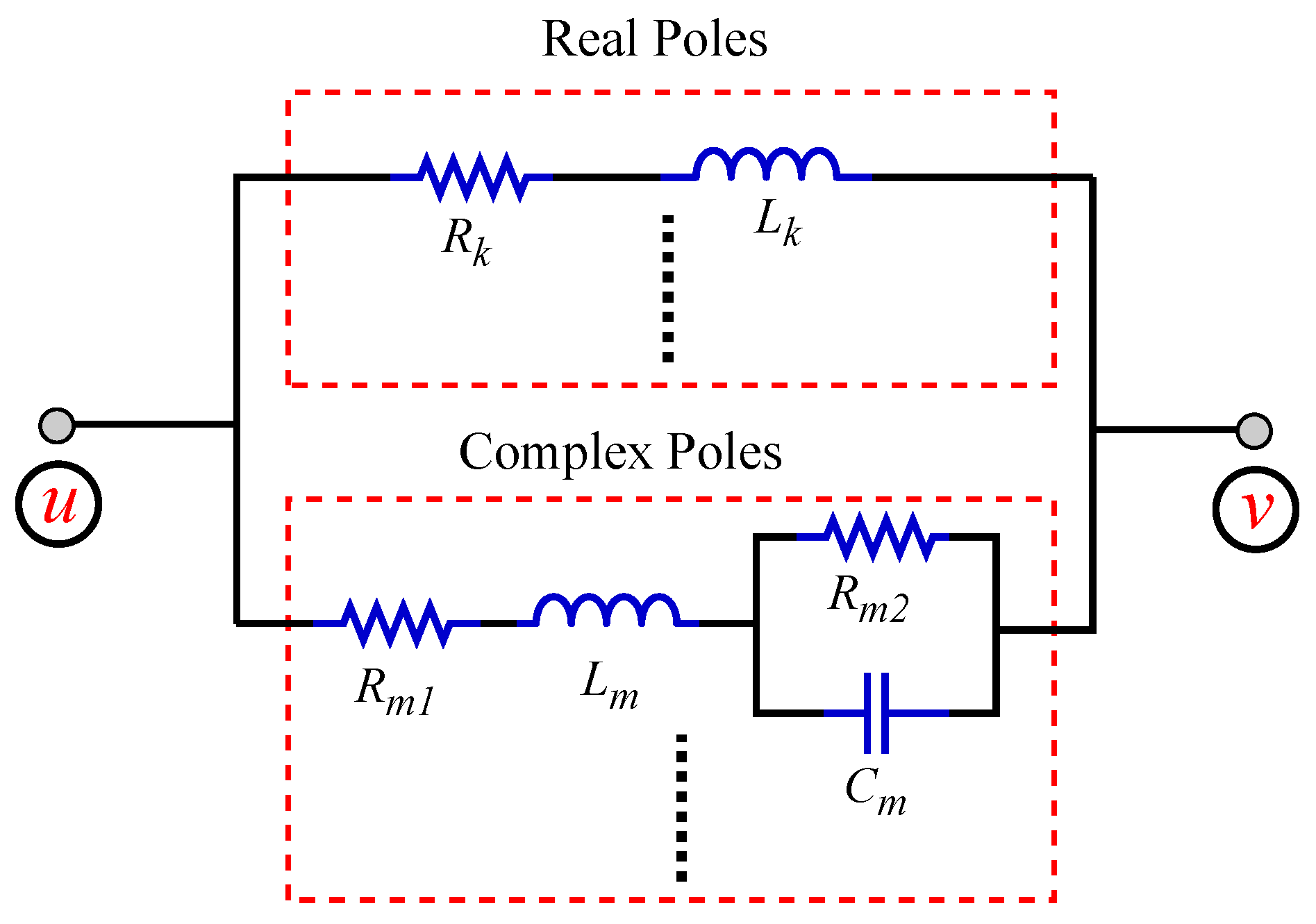
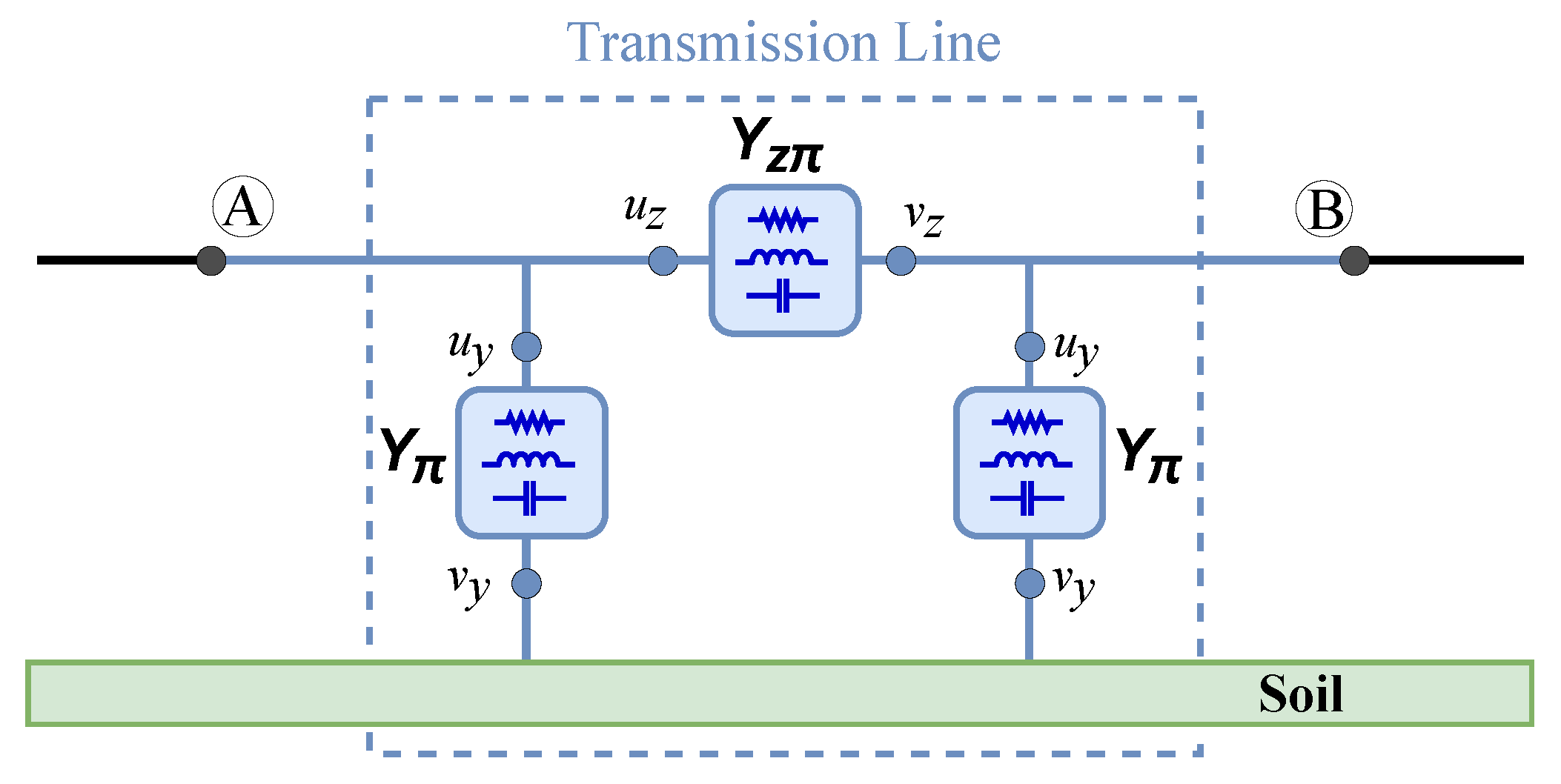
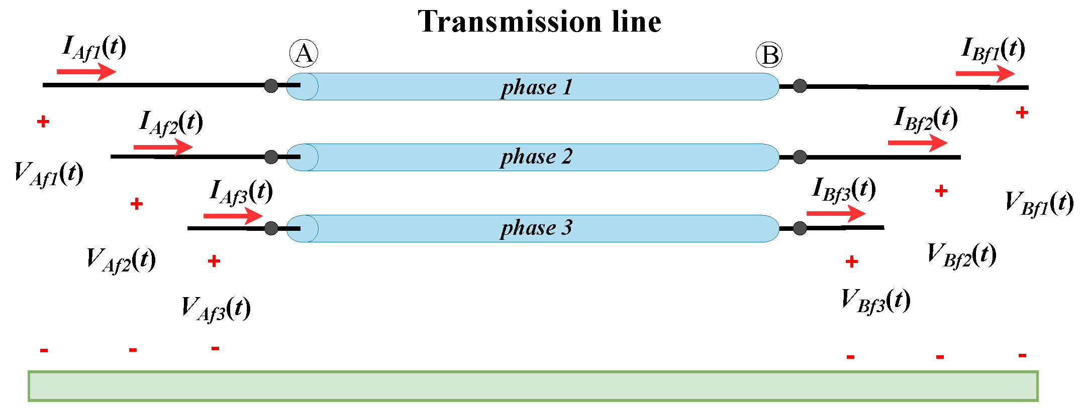
2. Exact Equivalent π-Circuit of a TL Formed by Circuit Elements

The circuit illustrated in Figure 1 represents the exact equivalent $\pi$-circuit of a TL. In this context, terminals A and B represent the sending and receiving of the line. The parameters $I_A$ and $I_B$ are the longitudinal currents, while the transverse voltages at these terminals are designated as $V_A$ and $V_B$. The exact equivalent $\pi$-circuit can be characterized by a series admittance, which is denoted as $Y_{z\pi }$. This admittance is linked between terminals A and B, along with a shunt admittance, and is designated as $Y_{\pi }$, which is connected to both terminals. Expressions (1) and (2) correspond to the admittance curves of $Y_{z\pi }$ and $Y_{\pi }$, respectively.

Figure 1. Representation of the transmission line through the exact equivalent $\pi$-circuit.

Figure 1. Representation of the transmission line through the exact equivalent $\pi$-circuit.

$$Y_{z\pi }\left(\omega \right)=\frac{1}{Z_c\left(\omega \right)sinh\left(\gamma \left(\omega \right)d\right)}$$

(1)

$$Y_{\pi }\left(\omega \right)=\frac{tanh\left(\gamma \right(\omega )d/2)}{Z_c\left(\omega \right)}$$

(2)

where $Z_c$($\omega$) and $\gamma$($\omega$) are the characteristic impedance and the propagation constant, as calculated from (3) and (4), respectively [22].

$$Z_c\left(\omega \right)=\sqrt{\frac{Z\left(\omega \right)}{Y\left(\omega \right)}}$$

(3)

$$\gamma \left(\omega \right)=\sqrt{Z\left(\omega \right)Y\left(\omega \right)}$$

(4)

In Equations (3) and (4), Z($\omega$) and Y($\omega$) represent the longitudinal impedance and transverse admittance of the line in pul, where $\omega$ = 2$\pi f$ is the angular frequency in rad/s, and f is the frequency in Hz.

$$Z\left(\omega \right)=R\left(\omega \right)+j\omega L\left(\omega \right)$$

(5)

$$Y\left(\omega \right)=G\left(\omega \right)+j\omega C\left(\omega \right)$$

(6)

It is observed that the exact equivalent $\pi$-circuit represents the single-phase TL while incorporating the frequency effect, that is, by considering the skin and soil effects on the conductor. However, this model can only be represented in the frequency domain [35]. Its representation in the time domain was recently proposed in [29]. This approach relies on the synthesis of the admittance curves of $Y_{z\pi }$ and $Y_{\pi }$ of the equivalent $\pi$-circuit, as shown in Figure 1; furthermore, this is achieved using only passive elements like resistors, inductors, and capacitors. The method consists of approximating the frequency domain admittance curves of $Y_{z\pi }$ and $Y_{\pi }$ using rational functions through the utilization of the vector fitting (VF) algorithm [36,37,38]. In the algorithm, the general rational function $F\left(s\right)$ in Equation (7) is employed to represent the frequency domain admittance curves of $Y_{z\pi }$ and $Y_{\pi }$, as explained in [39,40].

$$F\left(s\right)=\sum _{j=1}^{N_p}\left(\frac{r_j}{s-p_j}\right)+D+Es$$

(7)

where $r_j$ and $p_j$ denote the j-th residue and j-th pole, respectively, and with $N_p$ representing the number of poles and residues in the rational function. The term s corresponds to the complex angular frequency, while D and E are real coefficients, both of which are considered null in this study. The residues and poles can be either real or complex numbers, and they can result in two distinct types of functions, which form the partial fractions outlined in the general Equation (7). The rational function formed of real numbers is represented as $Y_r\left(s\right)$ in (8), and it corresponds to a series resistor–inductor (RL) circuit, as illustrated in Figure 2a. On the other hand, the other rational function is constructed using a pair of conjugate complex numbers, denoted as $Y_c\left(s\right)$ in (9), and it corresponds to an electrical circuit, as shown in Figure 2b [40].

$$Y_r\left(s\right)=\frac{r_k}{s-p_k}$$

(8)

$$Y_c\left(s\right)={\displaystyle \frac{r_m}{s-p_m}}+{\displaystyle \frac{r_m^{*}}{s-p_m^{*}}}$$

(9)

Expressions (10) and (11) were used to calculate the elements $R_k$ and $L_k$ of the equivalent RL circuit, as shown in Figure 2a. In turn, the Expressions (12) to (15) were used for the calculation of elements $R_{m1}$, $R_{m2}$, $L_m$, and $C_m$ of the equivalent RLC circuit, as shown in Figure 2b, respectively [41].

$$R_k=\frac{p_k}{r_k}$$

(10)

$$L_k=\frac{1}{r_k}$$

(11)

$$L_m=\frac{1}{r_m+r_m^{*}}$$

(12)

$$R_{m1}=-\frac{p_m{r}_m+p_m^{*}{r}_m^{*}}{2{r_m}^2}$$

(13)

$$C_m=\frac{{(r_m+r_m^{*})}^2}{r_m{r}_m^{*}{(p_m-p_m^{*})}^2}$$

(14)

$$R_{m2}=\frac{r_m+r_m^{*}}{C(p_m{r}_m^{*}+r_m{p}_m^{*})}$$

(15)

For each partial fraction that composes Equation (7), an equivalent electrical circuit branch was obtained. Figure 3 shows the connection of the RL and RLC branches, which are associated in parallel and synthesize the generic admittance that represents the rational function $F\left(s\right)$.

The connections of terminals u and v for the admittance curves of $Y_{z\pi }$ and $Y_{\pi }$ in representing the equivalent $\pi$-circuit of the TL are illustrated in Figure 4.

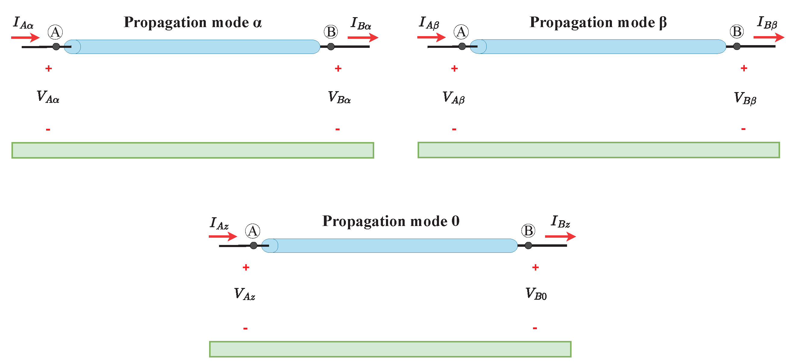
3. Representation of a Perfectly Transposed TL in the Mode Domain

We derived current and voltage equations for a three-phase TL, as shown in Figure 5, while considering the electromagnetic coupling among the phases; this is commonly achieved by expressing the line within the modal domain. In this context, the three-phase TL is represented through its three propagation modes, each of which behave like a single-phase TL, as shown in Figure 6.

The TL shown in Figure 5, when considered ideally transposed, is characterized by its longitudinal impedance matrix $\mathit{Z}$ and its transverse admittance matrix $\mathit{Y}$, which are written as shown in (16).

$$\mathit{Z}=\left[\begin{array}{ccc}{Z}_p& Z_m& Z_m\\ Z_m& Z_p& Z_m\\ Z_m& Z_m& Z_p\end{array}\right];\mathit{Y}=\left[\begin{array}{ccc}{Y}_p& Y_m& Y_m\\ Y_m& Y_p& Y_m\\ Y_m& Y_m& Y_p\end{array}\right]$$

(16)

The conversion from the phase domain to the modal domain is accomplished through a modal transformation matrix ${\mathit{T}}_{\mathit{v}}$. This matrix’s columns consist of the eigenvectors related to the eigenvalues that result from the matrix product $\mathit{Z}\mathit{Y}$, as described in [6]. Consequently, the matrices $\mathit{Z}$ and $\mathit{Y}$ are converted into the modal domain using Equation (17) [42,43].

$${\mathit{Z}}_{\mathit{mod}}=\mathit{T}{{}_{\mathit{v}}}^{-1}\mathit{Z}\mathit{T}{{}_{\mathit{v}}}^{-T};{\mathit{Y}}_{\mathit{mod}}=\mathit{T}{{}_{\mathit{v}}}^{-1}\mathit{Y}\mathit{T}{{}_{\mathit{v}}}^{-T}$$

(17)

In the context of a three-phase and ideally transposed TL, the Clarke matrix expressed in (18) can be used as the matrix ${\mathit{T}}_{\mathit{v}}$ [44].

$${\mathit{T}}_{\mathit{v}}=\left[\begin{array}{ccc}\frac{2}{\sqrt{6}}& 0& \frac{1}{\sqrt{3}}\\ -\frac{1}{\sqrt{3}}& \frac{1}{\sqrt{2}}& \frac{1}{\sqrt{3}}\\ -\frac{1}{\sqrt{6}}& -\frac{1}{\sqrt{2}}& \frac{1}{\sqrt{3}}\end{array}\right]$$

(18)

By substituting the matrix ${\mathit{T}}_{\mathit{v}}$ into Equation (17), one can derive the longitudinal impedance ${\mathit{Z}}_{\mathit{mod}}$ and the transverse admittance of the line ${\mathit{Y}}_{\mathit{mod}}$, which are both represented in the modal domain, as expressed in (19).

$${\mathit{Z}}_{\mathit{mod}}=\left[\begin{array}{ccc}{Z}_{\alpha }& 0& 0\\ 0& Z_{\beta }& 0\\ 0& 0& Z_0\end{array}\right];{\mathit{Y}}_{\mathit{mod}}=\left[\begin{array}{ccc}{Y}_{\alpha }& 0& 0\\ 0& Y_{\beta }& 0\\ 0& 0& Y_0\end{array}\right]$$

(19)

Hence, with the application of the Clarke matrix (18), both matrices $\mathit{Z}$ and $\mathit{Y}$ are decomposed into their precise modes. This approach considers the frequency influence on the TL parameters, regardless of the line’s geometry [4].

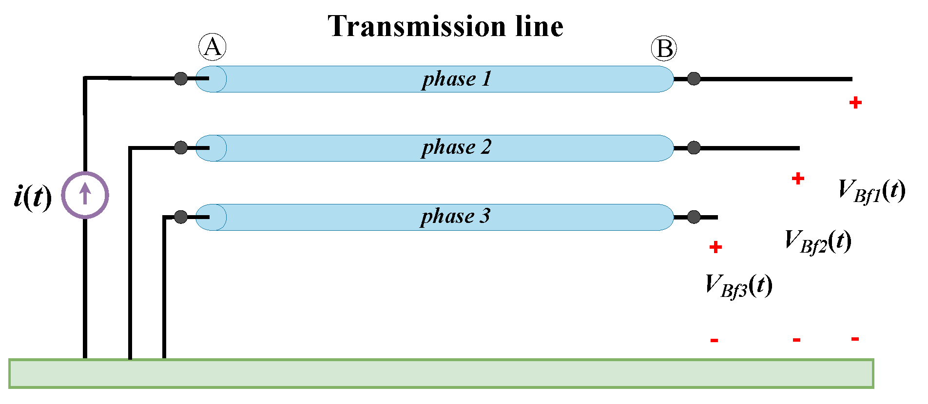
4. Representation of Propagation Modes Using the Exact Equivalent π Circuit

In order to use the exact equivalent $\pi$-circuit in the representation of three-phase lines, the TL represented in the phase domain, as shown in Figure 5, must be decomposed into three propagation modes, that is, $\alpha$, $\beta$, and zero, according to Figure 6. For each propagation mode, an admittance of $Y_{z\pi }$ and an admittance of $Y_{\pi }$ are obtained, which will compose the exact equivalent $\pi$-circuit of the respective mode, as shown in Figure 7. The admittance of $Y_{z\pi }$ for the modes $\alpha$, $\beta$, and zero are obtained from (20), (21), and (22), respectively. The admittance of $Y_{\pi }$ for modes $\alpha$, $\beta$, and zero are obtained from (23), (24), and (25), respectively.

Figure 7. Representation of the propagation modes through exact equivalent $\pi$-circuits.

Figure 7. Representation of the propagation modes through exact equivalent $\pi$-circuits.

$$Y_{z\pi \alpha }\left(\omega \right)=\frac{1}{Z_{c\alpha }\left(\omega \right)sinh\left({\gamma }_{\alpha }\left(\omega \right)d\right)}$$

(20)

$$Y_{z\pi \beta }\left(\omega \right)=\frac{1}{Z_{c\beta }\left(\omega \right)sinh\left({\gamma }_{\beta }\left(\omega \right)d\right)}$$

(21)

$$Y_{z\pi 0}\left(\omega \right)=\frac{1}{Z_{c0}\left(\omega \right)sinh\left({\gamma }_0\left(\omega \right)d\right)}$$

(22)

$$Y_{\pi \alpha }\left(\omega \right)=\frac{tanh({\gamma }_{\alpha }\left(\omega \right)d/2)}{Z_{c\alpha }\left(\omega \right)}$$

(23)

$$Y_{\pi \beta }\left(\omega \right)=\frac{tanh({\gamma }_{\beta }\left(\omega \right)d/2)}{Z_{c\beta }\left(\omega \right)}$$

(24)

$$Y_{\pi 0}\left(\omega \right)=\frac{tanh({\gamma }_0\left(\omega \right)d/2)}{Z_{c0}\left(\omega \right)}$$

(25)

All of the admittance curves of $Y_{z\pi }$ and $Y_{\pi }$ for the three propagation modes are synthesized by circuit elements, and this is achieved using the technique described in Section 2. Thus, one can represent each propagation mode by an exact equivalent $\pi$-circuit, which is formed by circuit elements.

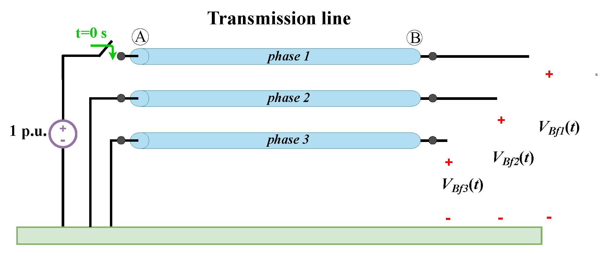
5. Methodology for the Implementation of a Proposed Model in ATP Software

In the implementation of the three-phase model in circuit simulation programs such as ATP, the transformation of voltages and currents from the phase domain to the modal one, and vice-versa, is performed with the use of an arrangement of ideal transformers, as described in [5]. In this method, each ideal transformer’s turns ratio and polarity represent a Clarke matrix component in Equation (18). Figure 8 shows the generic implementation of the three-phase model in ATPDraw software (version 7.0p7).

The ideal transformers connected at end A result in the phase-to-mode and mode-to-phase transformations at the sending end of the line. In the same way, the ideal transformers connected at end B perform the mode-to-phase and phase-to-mode transformations at the receiving end. For each propagation mode of the TL, the circuits formed by the admittance curves of $Y_{z\pi }$ and $Y_{\pi }$ can be implemented in ATPDraw software by manually inserting the RLC circuits, or by creating a routine to automate and generate the RLC circuits within the LIB component, as shown in [29,45]. In this work, the LIB component was used.

Thus, the simulations of the three-phase model were carried out entirely in circuit simulation programs, in which voltages and currents were simultaneously available in the phase and modal domains.

Figure 8. Implementation of proposed model in the ATPDraw software.

Figure 8. Implementation of proposed model in the ATPDraw software.

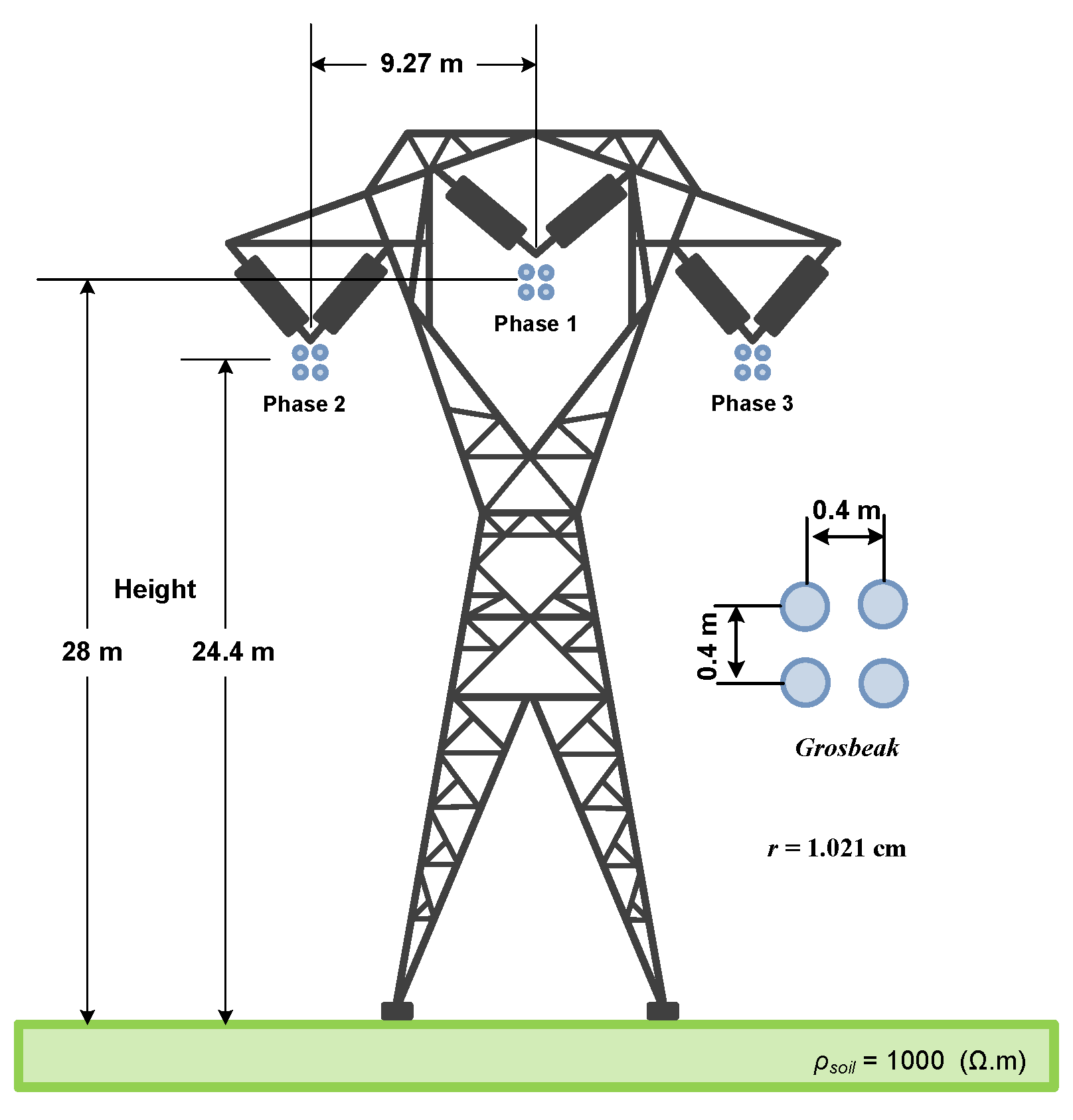
6. Results and Discussion

The simulation results were obtained by considering a TL with the profile shown in Figure 9. Each phase (1, 2, and 3) comprised four conductors, each with a radius of 1.021 cm, a spacing of 0.40 m, and a resistivity of 0.0799 Ω/km. The soil resistivity was assumed to be 1000 Ω·m. Longitudinal parameters were calculated by considering the soil and skin effects, with frequency values varying between 0.1 Hz and 100 kHz.

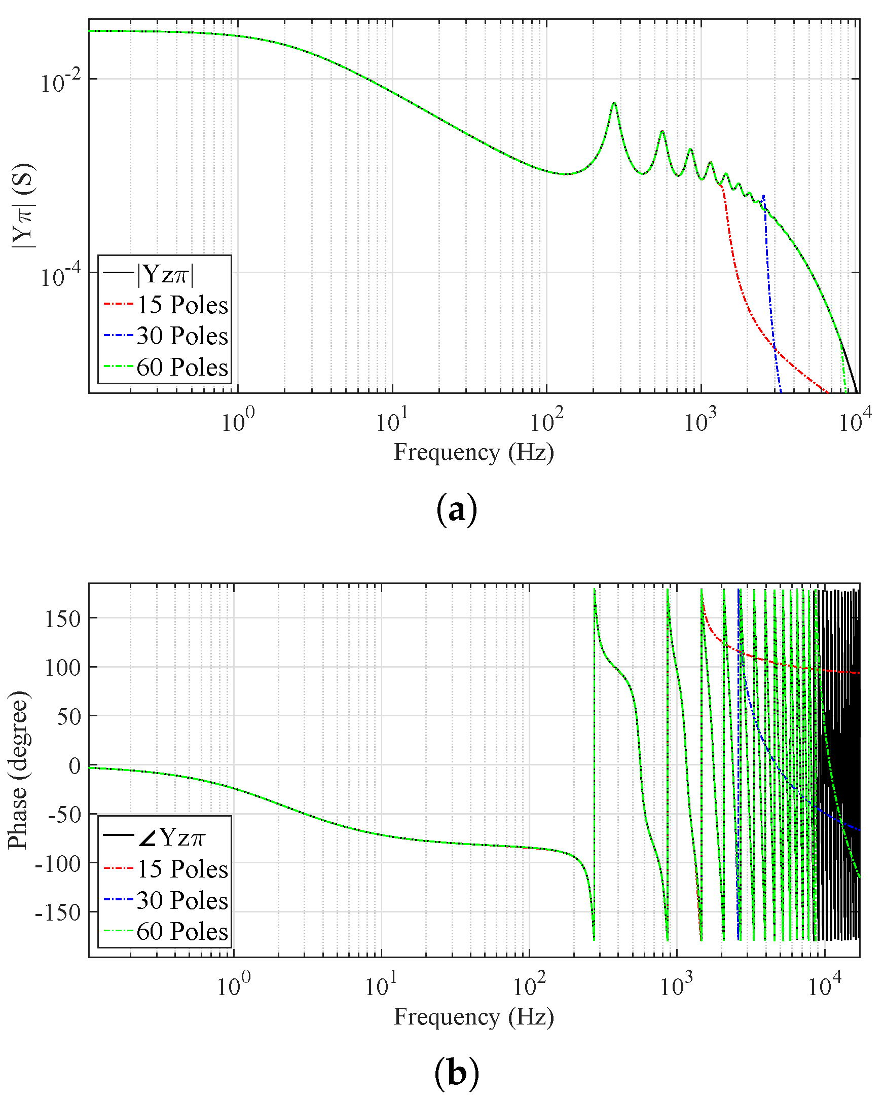
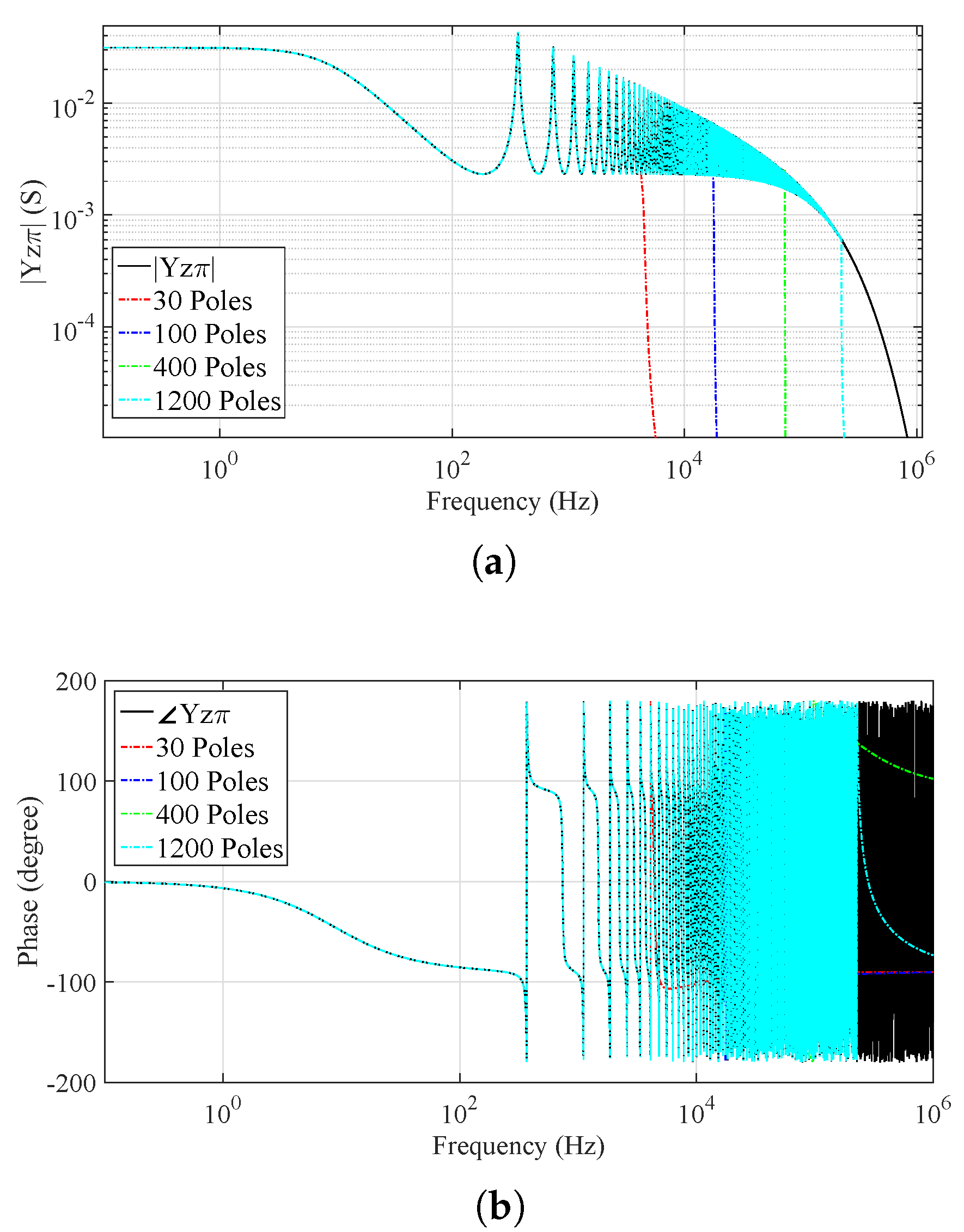
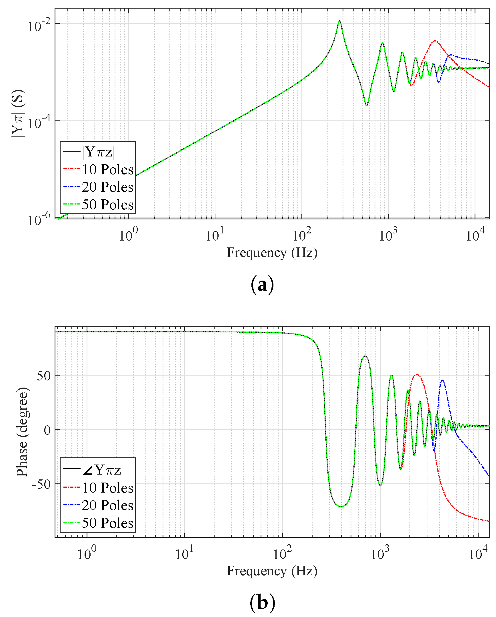
6.1. Rational Approximation of the Admittance Curves of $Y_{z\pi }$ and $Y_{\pi }$ in the Propagation Modes

The admittance curves of $Y_{z\pi }$ and $Y_{\pi }$ for the three propagation modes were obtained for a TL of 400 km. The number of poles used to approximate the two admittance curves and their respective propagation modes are shown in

Table 1. The number of poles for the settings of $Y_{z\pi }$ and $Y_{\pi }$ for the propagation modes.

Poles
	Modes $\mathit{\alpha }$ and $\mathit{\beta }$		Mode 0
Settings	${\mathit{Y}}_{\mathit{z}\mathit{\pi }}$	${\mathit{Y}}_{\mathit{\pi }}$	${\mathit{Y}}_{\mathit{z}\mathit{\pi }}$	${\mathit{Y}}_{\mathit{\pi }}$
1	30	20	60	50
2	100	80	60	50
3	400	260	60	50
4	1200	570	60	50

.

Figure 10 shows the magnitude and phase of the exact admittance of $Y_{z\pi }$ for the modes $\alpha$ and $\beta$, which correspond to $Y_{z\pi \alpha }$ and $Y_{z\pi \beta }$, respectively, as well as with the curves that represent their approximate functions with 30, 100, 400, and 1200 poles. According to Table 1, the numbers of poles were chosen randomly but in ascending order (up to 1200 poles), whereas the curve was adjusted until the end of the resonance peaks. It was observed that the curve with 400 poles overlapped with the reference value over a wide range of frequencies. In turn, it did not match the reference for frequencies at which the magnitude of admittance $Y_{z\pi \alpha }$ was already more attenuated.

The zero-mode admittance $Y_{z\pi 0}$ presented few resonance peaks. Consequently, the number of poles used to perform the rational approximation was much smaller, as seen in Figure 11. This plot shows the magnitude and phase for the zero mode of the exact admittance $Y_{z\pi 0}$, as well as for the curves of their approximate functions with 15, 30, and 60 poles.

Figure 12 shows the magnitude and phase of the exact admittance curves of $Y_{\pi \alpha }$ and $Y_{\pi \beta }$ for the $\alpha$ and $\beta$ propagation modes, as well as for the curves of their approximate functions with 20, 80, 260, 570, and 1500 poles. The numbers of poles were chosen according to those that could adjust the admittance of $Y_{\pi }$, and the number chosen was the amount necessary to adjust $Y_{\pi }$ to the same frequency ranges as the admittance of $Y_{z\pi }$. It was observed that the adjusted curve with 1500 poles overlapped with the reference value until the end of the resonance peaks.

Figure 11. Admittance $Y_{z\pi }$ of the zero mode: (a) Magnitude. (b) Phase.

Figure 11. Admittance $Y_{z\pi }$ of the zero mode: (a) Magnitude. (b) Phase.

Figure 12. Admittance $Y_{\pi }$ of the $\alpha$ and $\beta$ modes: (a) Magnitude. (b) Phase.

Figure 12. Admittance $Y_{\pi }$ of the $\alpha$ and $\beta$ modes: (a) Magnitude. (b) Phase.

Figure 13 shows the magnitude and phase of the exact admittance for the zero mode, $Y_{\pi 0}$, as well as for the curves of its functions that were approximated with 10, 20, and 50 poles. It was observed that the admittance of $Y_{\pi 0}$ required a much smaller number of poles for the approximation, as did the zero-mode admittance of $Y_{z\pi 0}$.

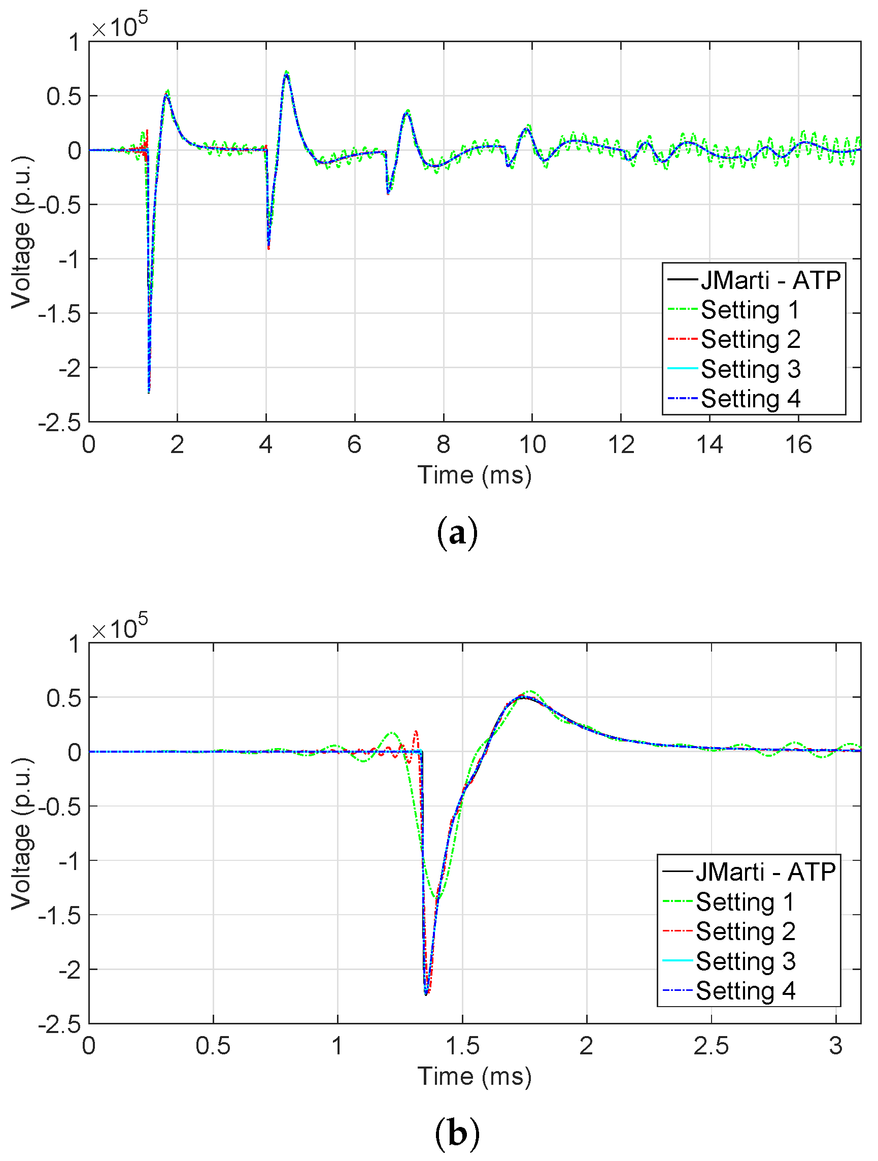
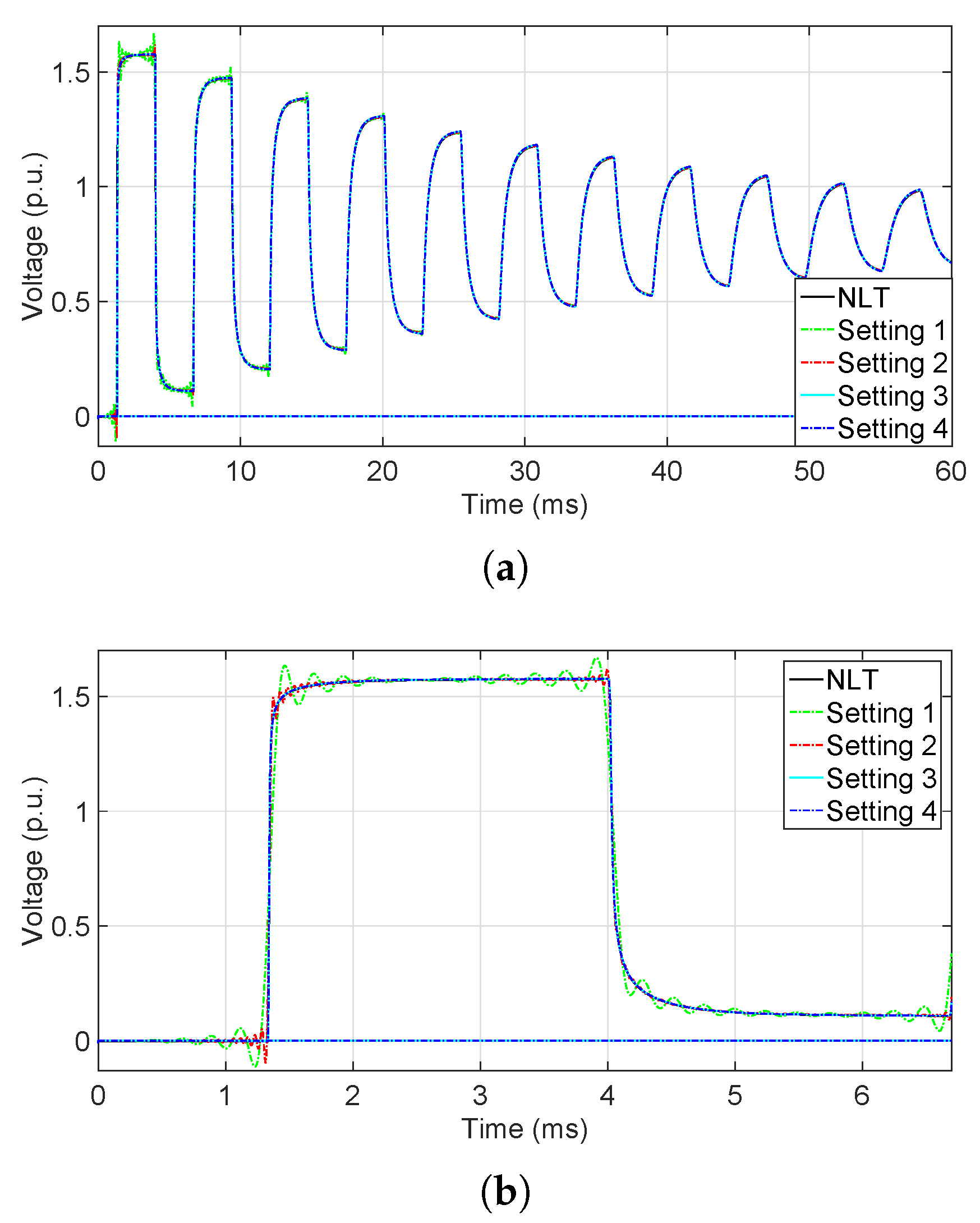
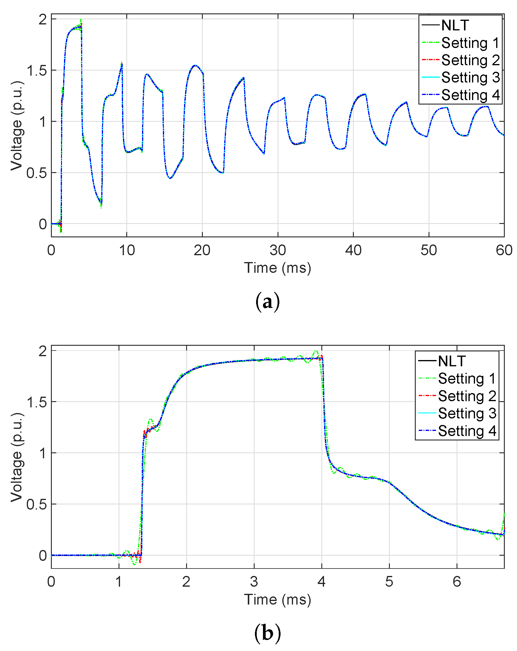
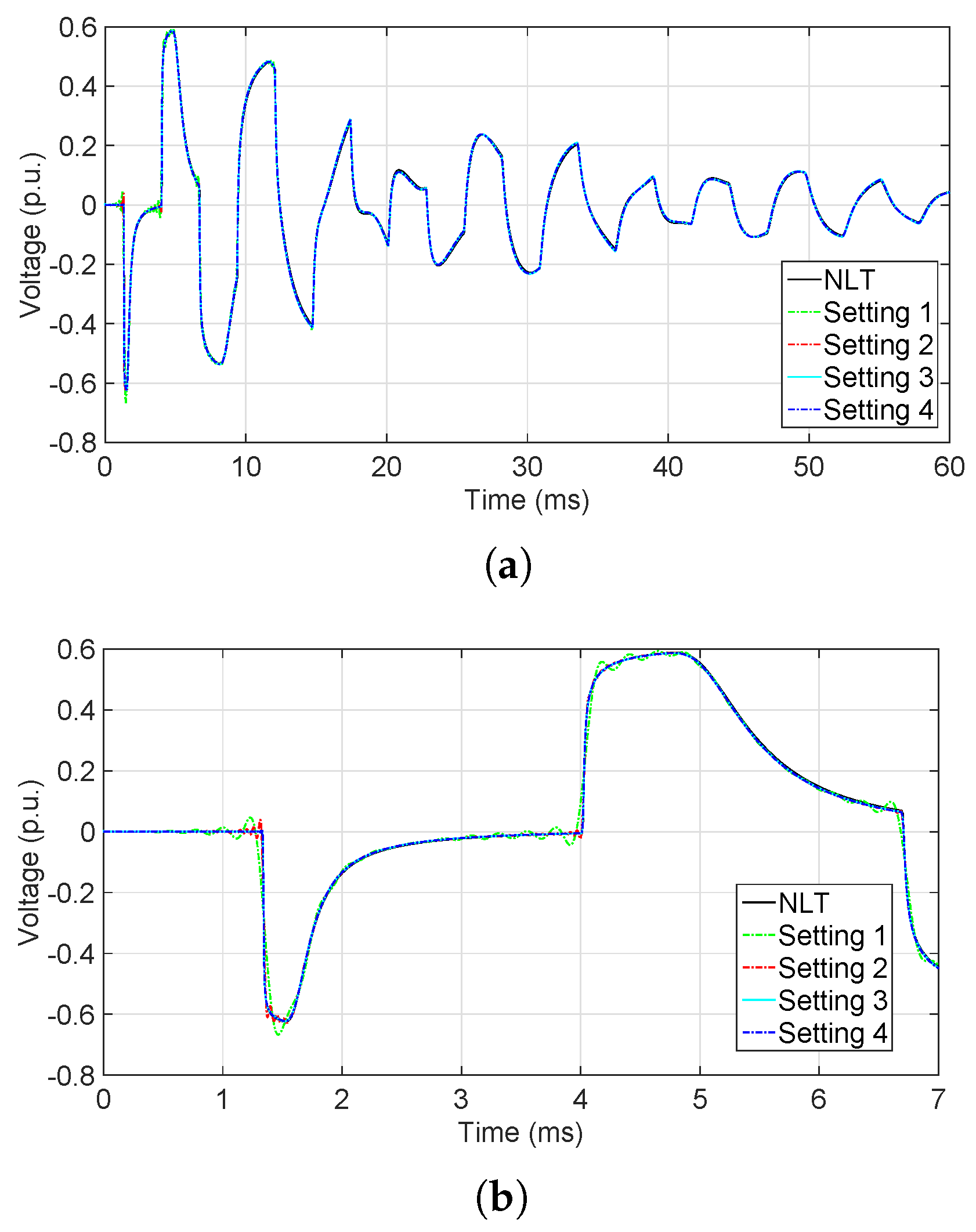
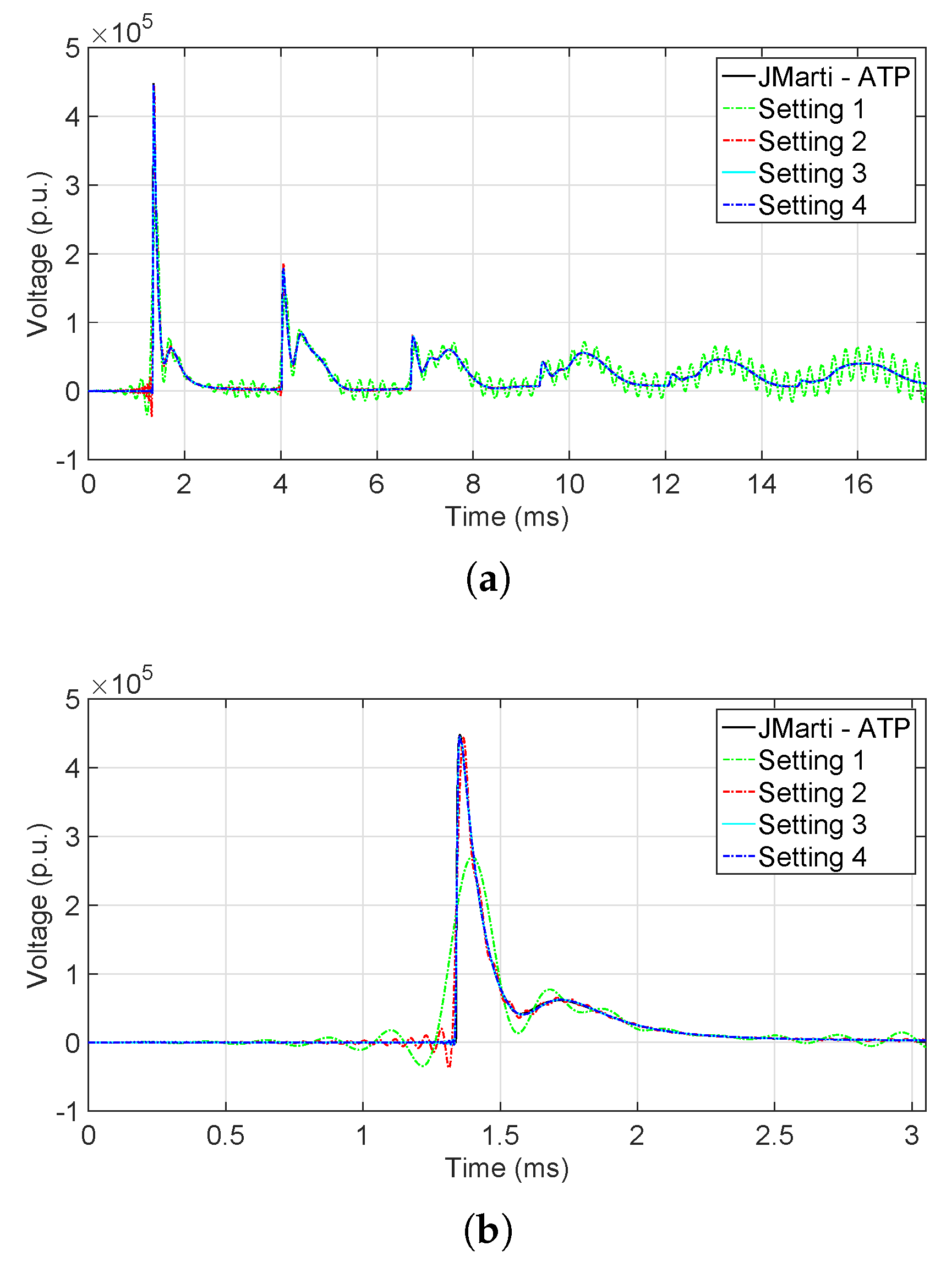
6.2. Time-Domain Analysis

The three-phase TL formed by circuit elements was implemented and simulated within the ATP/ATPDraw environment to analyze the transients in the time domain. From the approximate admittance curves of the 400 km three-phase TL defined in Section 6.1, the equivalent $\pi$-circuits were formed for each propagation mode, and they were synthesized with the number of poles shown in Table 1.

The simulation in ATP/ATPDraw was performed using a notebook with an Intel^® i7-3630QM processor (Intel, Sao Paulo, Brazil) and 4 GB of random access memory (RAM) while always considering a time step $\Delta t=0.1\mathsf{\mu }\mathrm{s}$. Despite the huge amount of circuit elements, the simulation time for setting 3 (400 poles) was around one minute, whereas for setting 4 (1200 poles) it was around three minutes. Settings 1 and 2 took around 20 s and 45 s, respectively.

6.2.1. Low-Frequency Analysis

The low-frequency transient simulations were initiated by energizing the line with a DC voltage source of 1 pu. When a switch connected to the sending end of the TL was closed at t = 0 s, only phase 1 was connected, while phases 2 and 3 were short-circuited. The receiving end of the line was left open, as illustrated in Figure 14. To assess the results obtained with the proposed model, reference values were calculated utilizing the NLT.

Figure 15 shows the voltages at the receiving ends, specifically $V_{B\alpha }$(t) and $V_{B\beta }$(t) for the $\alpha$ and $\beta$ modes in the time domain, respectively. In both cases, the reference voltage was computed using the NLT, and it was then compared with the corresponding voltage, $V_{B\beta }$(t), which was obtained from the ATP/ATPDraw software. The voltages in the $\beta$ mode, that is, $V_{B\beta }$(t) were zero.

Despite the significant difference in the number of poles between settings 1 and 4, Figure 15 evidences that the difference between the voltage curves for those two settings in the $\alpha$ mode was insignificant.

Figure 16 shows the voltage at the receiving end of the zero mode in the time domain that corresponded to $V_{B0}$(t), as well as to the voltages obtained by simulating the novel model in ATP/ATPDraw. According to Table 1, all settings have the same number of poles, thus leading to identical results. The same number of poles was used because, with only a few poles, the settings achieved an excellent result during the transient analysis. As such, this strategy was adopted in the study to analyze only the influence of the $\alpha$ and $\beta$ modes on the voltage results in the phase domain, and this was performed because the number of poles used in these propagation modes was much larger.

Figure 17 and Figure 18 show the voltages at the receiving end in the phase domain. From the analysis of the curves, it is possible to observe that, for setting 1, the distortions in the phase domain are not so severe, despite the small number of poles compared to setting 4. Setting 3 already presents an excellent result for low-frequency transients. It was observed that the voltages $V_{Bf1}$(t) and $V_{Bf2}$(t) did not have distortions in the case of setting 4; this was also especially the case for setting 3, which was not adjusted until the end of the resonance peaks for the admittance of $Y_{z\pi }$. The curve obtained with setting 3 was found to be identical to that of setting 4 and the reference curve.

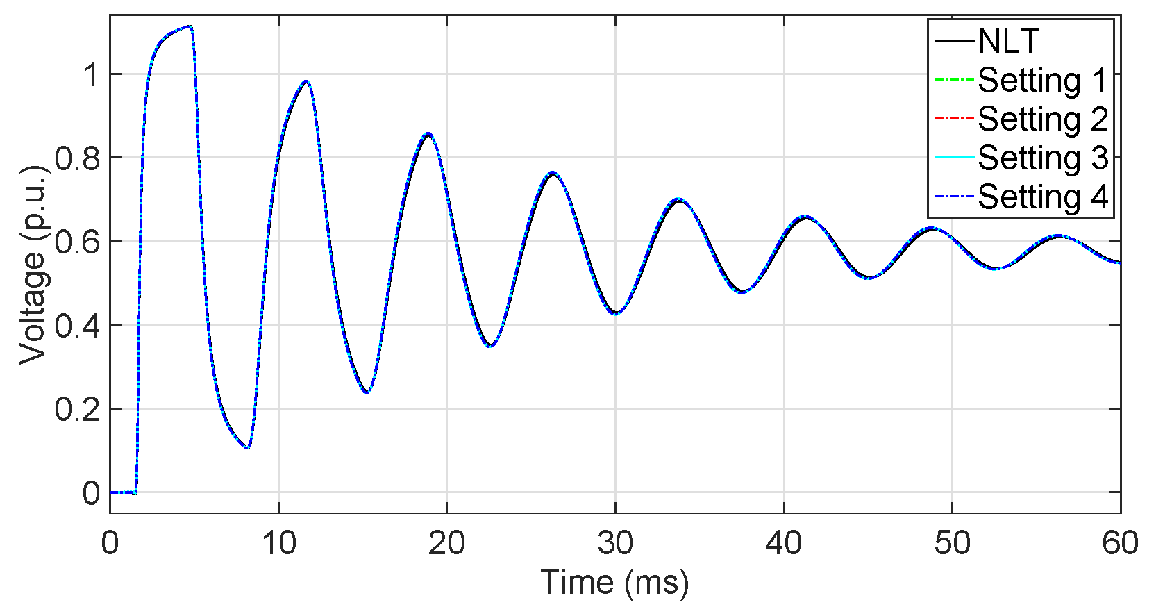
6.2.2. High-Frequency Analysis

The electromagnetic transients at higher frequencies result by applying an atmospheric impulse to phase 1 at the sending end of the TL. In contrast, phases 2 and 3 remain short-circuited, and the receiving end of the line is left open, as depicted in Figure 19.

Lightning is characterized by a current source that represents a double exponential function with an amplitude of 1 kA, a front time of 1.20 µs, and a tail time of 50 µs [46]. When considering a three-phase TL of 400 km, the equivalent $\pi$-circuits were synthesized with the number of poles according to Table 1.

J. Marti’s model was chosen as a reference benchmark for all the simulation results in ATP/ATPDraw. Figure 20 shows the voltage at the receiving end at phase 1. Figure 21 represents the voltages at the receiving ends of phases 2 and 3, which had the same behavior. The curve corresponding to setting 1 denoted the behavior of a model that used only a few poles, and which, consequently, had a distorted response.

The difference between the other settings is easier to observe in Figure 20b and Figure 21b. Even with a much smaller number of poles, the curve for Setting 2 produced a very satisfactory result. The curves for settings 3 and 4 overlapped with the reference value. This behavior evidences that, with the number of poles used in setting 3, it is already possible to obtain an excellent high-frequency response for the three-phase TL when using the proposed model.

Figure 21. Open-circuit voltage at the receiving end of phases 2 and 3 during an atmospheric impulse event: (a) transient behavior up to t = 16 ms; (b) occurrence of the first reflection wave.

Figure 21. Open-circuit voltage at the receiving end of phases 2 and 3 during an atmospheric impulse event: (a) transient behavior up to t = 16 ms; (b) occurrence of the first reflection wave.

7. Conclusions

This paper presents a novel model for representing the perfectly transposed three-phase transmission lines in the time domain. The model, developed in the modal domain, was obtained from synthesizing the exact equivalent $\pi$-circuit for each propagation mode, which was achieved using a combination of discrete passive elements. The model considers the distributed parameters of the transmission line and considers the frequency dependence in the line. In other words, the calculation of longitudinal parameters incorporates skin effects and soil influences. Moreover, in addition to considering constant soil parameters, the proposed model allows for the inclusion of frequency-dependent soil electrical parameters. The synthesis process employs the vector fitting (VF) technique to obtain the poles and zeros of the rational functions that approximate the admittance curves of $Y_{z\pi }$ and $Y_{\pi }$, which are of the respective exact, equivalent $\pi$-circuits.

The main disadvantage of the proposed model is the presence of numerous resonance peaks in propagation modes $\alpha$ and $\beta$, which necessitates a high number of poles and, consequently, a larger number of circuit elements for synthesizing the equivalent $\pi$-circuit. Nevertheless, the required simulation time interval in ATP/ATPDraw remains manageable.

The proposed model was tested by considering electromagnetic transients composed of a wide range of frequencies, thus leading to accurate results. By modeling the transmission line using only ideal transformers and linear circuit elements, one can implement the model in most electrical circuit simulation software, and this is achieved using time-varying elements to simulate the transmission lines.

In summary, the novel approach incorporates the essential characteristics of the exact, equivalent $\pi$-circuit by accounting for distributed and frequency-dependent parameters. The primary advantage lies in the ability to simulate electromagnetic transients directly in the time domain, thus obviating the need for calculating the propagation time $\tau$ in advance, and thus not requiring a resort to complex mathematical operations such as convolutions, inverse Laplace transforms, or Fourier transforms.

Future work will include optimizing the simultaneous adjustment of the admittance curves of $Y_{z\pi }$ and $Y_{z\pi }$ through a more in-depth study, all the while considering the maximum frequencies of adjustment by aiming at reducing the number of poles and, consequently, the number of circuit elements used in the model. Additionally, there is an intention to extend the model’s applicability to encompass non-transposed and asymmetric transmission lines. Finally, the plan is to compare the proposed model with experimental results, as was presented in [17].

References

1. Morched, A.; Gustavsen, B.; Tartibi, M. A universal model for accurate calculation of electromagnetic transients on overhead lines and underground cables. IEEE Trans. Power Deliv. 1999, 14, 1032–1038. [Google Scholar] [CrossRef]
2. Vega, M.G.; Naredo, J.; Ramos-Leaños, O. Minimum Delay Systems for the Modeling of Transmission Lines at EMT Power System Studies. Signal 2017, 10, 11. [Google Scholar]
3. Kocar, I.; Mahseredjian, J. New procedure for computation of time delays in propagation function fitting for transient modeling of cables. IEEE Trans. Power Deliv. 2015, 31, 613–621. [Google Scholar] [CrossRef]
4. Torrez Caballero, P.; Marques Costa, E.C.; Kurokawa, S. Modal decoupling of overhead transmission lines using real and constant matrices: Influence of the line length. Int. J. Electr. Power Energy Syst. 2017, 92, 202–211. [Google Scholar] [CrossRef]
5. Colqui, J.S.L.; Eraso, L.C.T.; Caballero, P.T.; Pissolato Filho, J.; Kurokawa, S. Implementation of Modal Domain Transmission Line Models in the ATP Software. IEEE Access 2022, 10, 15924–15934. [Google Scholar] [CrossRef]
6. Wedepohl, L.; Nguyen, H.; Irwin, G. Frequency-dependent transformation matrices for untransposed transmission lines using Newton-Raphson method. IEEE Trans. Power Syst. 1996, 11, 1538–1546. [Google Scholar] [CrossRef]
7. Nguyen, T.; Chan, H. Evaluation of modal transformation matrices for overhead transmission lines and underground cables by optimization method. IEEE Trans. Power Deliv. 2002, 17, 200–209. [Google Scholar] [CrossRef]
8. Chrysochos, A.I.; Papadopoulos, T.A.; Papagiannis, G.K. Robust Calculation of Frequency-Dependent Transmission-Line Transformation Matrices Using the Levenberg–Marquardt Method. IEEE Trans. Power Deliv. 2014, 29, 1621–1629. [Google Scholar] [CrossRef]
9. Uribe, F.A.; Naredo, J.L.; Moreno, P.; Guardado, L. Electromagnetic transients in underground transmission systems through the numerical Laplace transform. Int. J. Electr. Power Energy Syst. 2002, 24, 215–221. [Google Scholar] [CrossRef]
10. Moreno, P.; Ramirez, A. Implementation of the Numerical Laplace Transform: A Review Task Force on Frequency Domain Methods for EMT Studies. IEEE Trans. Power Deliv. 2008, 23, 2599–2609. [Google Scholar] [CrossRef]
11. Alameri, H.A.; Gomez, P. Laplace Domain Modeling of Power Components for Transient Converter-Grid Interaction Studies. In Proceedings of the 2021 North American Power Symposium (NAPS), College Station, TX, USA, 14–16 November 2021; pp. 1–6. [Google Scholar] [CrossRef]
12. Camara, F.; Lima, A.C.; Correia de Barros, M.T.; da Silva, F.F.; Bak, C.L. Admittance-based modelling of cables and overhead lines by idempotent decomposition. Electr. Power Syst. Res. 2023, 224, 109596. [Google Scholar] [CrossRef]
13. Mikulović, J.Č.; Šekara, T.B. The numerical method of inverse Laplace transform for calculation of overvoltages in power transformers and test results. Serbian J. Electr. Eng. 2014, 11, 243–256. [Google Scholar] [CrossRef]
14. Mamiş, M. Computation of electromagnetic transients on transmission lines with nonlinear components. IEE Proc.-Gener. Transm. Distrib. 2003, 150, 200–204. [Google Scholar] [CrossRef]
15. Marti, L. Simulation of transients in underground cables with frequency-dependent modal transformation matrices. IEEE Trans. Power Deliv. 1988, 3, 1099–1110. [Google Scholar] [CrossRef]
16. De Conti, A.; Emídio, M.P.S. Extension of a modal-domain transmission line model to include frequency-dependent ground parameters. Electr. Power Syst. Res. 2016, 138, 120–130. [Google Scholar] [CrossRef]
17. Challa, K.K.; Gurrala, G. Development of an Experimental Scaled-Down Frequency Dependent Transmission Line Model. IEEE Access 2021, 9, 64639–64652. [Google Scholar] [CrossRef]
18. Macias, J.R.; Exposito, A.G.; Soler, A.B. A comparison of techniques for state-space transient analysis of transmission lines. IEEE Trans. Power Deliv. 2005, 20, 894–903. [Google Scholar] [CrossRef]
19. Kurokawa, S.; Yamanaka, F.N.; Prado, A.J.; Pissolato, J. Inclusion of the frequency effect in the lumped parameters transmission line model: State space formulation. Electr. Power Syst. Res. 2009, 79, 1155–1163. [Google Scholar] [CrossRef]
20. Araujo, A.; Silva, R.; Kurokawa, S. Comparing lumped and distributed parameters models in transmission lines during transient conditions. In Proceedings of the 2014 IEEE Pes T&d Conference and Exposition, Chicago, IL, USA, 14–17 April 2014; pp. 1–5. [Google Scholar]
21. Ametani, A. Electromagnetic transients program: History and future. IEEJ Trans. Electr. Electron. Eng. 2021, 16, 1150–1158. [Google Scholar] [CrossRef]
22. Martí, J.R. Accurate Modeling of Frequency-Dependent Transmission Lines in Electromagnetic Transient Simulations. IEEE Power Eng. Rev. 1982, PER-2, 29–30. [Google Scholar] [CrossRef]
23. Caballero, P.T.; Costa, E.C.M.; Kurokawa, S. Frequency-dependent line model in the time domain for simulation of fast and impulsive transients. Int. J. Electr. Power Energy Syst. 2016, 80, 179–189. [Google Scholar] [CrossRef]
24. Bode, H.W. Network Analysis and Feedback Amplifier Design; D.V. Nostrand: New York, NY, USA, 1945. [Google Scholar]
25. Bañuelos-Cabral, E.; Gutiérrez-Robles, J.; García-Sánchez, J.; Sotelo-Castañón, J.; Galván-Sánchez, V. Accuracy enhancement of the JMarti model by using real poles through vector fitting. Electr. Eng. 2019, 101, 635–646. [Google Scholar] [CrossRef]
26. Colqui, J.S.L.; Araújo, A.R.J.D.; Pascoalato, T.F.G.; Kurokawa, S.; Filho, J.P. Transient Analysis on Multiphase Transmission Line Above Lossy Ground Combining Vector Fitting Technique in ATP Tool. IEEE Access 2022, 10, 86204–86214. [Google Scholar] [CrossRef]
27. De Lauretis, M.; Ekman, J.; Antonini, G.; Romano, D. Enhanced delay-rational Green’s method for cable time domain analysis. In Proceedings of the 2015 International Conference on Electromagnetics in Advanced Applications (ICEAA), Turin, Italy, 7–11 September 2015; pp. 1228–1231. [Google Scholar] [CrossRef]
28. Gustavsen, B. Optimal time delay extraction for transmission line modeling. IEEE Trans. Power Deliv. 2016, 32, 45–54. [Google Scholar] [CrossRef]
29. Balestero, P.J.R.; Colqui, J.S.L.; Kurokawa, S. Using the Exact Equivalent π-Circuit of Transmission Lines for Electromagnetic Transient Simulations in the Time Domain. IEEE Access 2022, 10, 90847–90856. [Google Scholar] [CrossRef]
30. Singh, A.; Marti, J.R.; Srivastava, K.D. Algorithms for fast simulation of transformer windings for diagnostic testing of power transformers. IEEE Trans. Power Deliv. 2010, 25, 1564–1572. [Google Scholar] [CrossRef]
31. Dommel, H.W. EMTP Theory Book; Microtran Power System Analysis Corporation: Vancouver, BC, Canada, 1996. [Google Scholar]
32. Portela, C.; Tavares, M. Modeling, simulation and optimization of transmission lines. Applicability and limitations of some used procedures. In Proceedings of the 2002 Transmission and Distribution Latin America Conference, Sao Paulo, Brazil, 18–22 March 2002. [Google Scholar]
33. Glover, J.D.; Sarma, M.S.; Overbye, T. Power System Analysis & Design, SI Version; Cengage Learning: Boston, MA, USA, 2012. [Google Scholar]
34. Paul, C.R. Decoupling the multiconductor transmission line equations. IEEE Trans. Microw. Theory Tech. 1996, 44, 1429–1440. [Google Scholar] [CrossRef]
35. Marti, J.; Marti, L.; Dommel, H. Transmission line models for steady-state and transients analysis. In Proceedings of the Joint International Power Conference Athens Power Tech, Athens, Greece, 5–8 September 1993; Volume 2, pp. 744–750. [Google Scholar]
36. Gustavsen, B.; Semlyen, A. Rational approximation of frequency domain responses by vector fitting. IEEE Trans. Power Deliv. 1999, 14, 1052–1059. [Google Scholar] [CrossRef]
37. Deschrijver, D.; Mrozowski, M.; Dhaene, T.; De Zutter, D. Macromodeling of multiport systems using a fast implementation of the vector fitting method. IEEE Microw. Wirel. Compon. Lett. 2008, 18, 383–385. [Google Scholar] [CrossRef]
38. Gustavsen, B. Improving the pole relocating properties of vector fitting. IEEE Trans. Power Deliv. 2006, 21, 1587–1592. [Google Scholar] [CrossRef]
39. Gustavsen, B.; Semlyen, A. Enforcing passivity for admittance matrices approximated by rational functions. IEEE Trans. Power Syst. 2001, 16, 97–104. [Google Scholar] [CrossRef]
40. Gustavsen, B. Computer code for rational approximation of frequency dependent admittance matrices. IEEE Trans. Power Deliv. 2002, 17, 1093–1098. [Google Scholar] [CrossRef]
41. Antonini, G. SPICE equivalent circuits of frequency-domain responses. IEEE Trans. Electromagn. Compat. 2003, 45, 502–512. [Google Scholar] [CrossRef]
42. Budner, A. Introduction of Frequency-Dependent Line Parameters into an Electromagnetic. IEEE Trans. Power Appar. Syst. 1970, PAS-89, 88–97. [Google Scholar] [CrossRef]
43. Portela, C.; Tavares, M. Six-phase transmission line-propagation characteristics and new three-phase representation. IEEE Trans. Power Deliv. 1993, 8, 1470–1483. [Google Scholar] [CrossRef]
44. Clarke, E. Circuit Analysis of A–C Power Systems: Graph. Darst; Wiley: Hoboken, NJ, USA, 1950. [Google Scholar]
45. Sajid Leon Colqui, J.; Carlos Timaná, L.; Kurokawa, S.; Ricardo Justo De Araújo, A.; Pissolato Filho, J. Lightning Current on the Frequency-Dependent Lumped Parameter Model Representing Short Transmission Lines. In Proceedings of the 2021 35th International Conference on Lightning Protection (ICLP) and XVI International Symposium on Lightning Protection (SIPDA), Colombo, Sri Lanka, 20–26 September 2021; Volume 1, pp. 1–8. [Google Scholar] [CrossRef]
46. Jia, W.; Xiaoqing, Z. Double-exponential expression of lightning current waveforms. In Proceedings of the 2006 4th Asia-Pacific Conference on Environmental Electromagnetics, Dalian, China, 1–4 August 2006; pp. 320–323. [Google Scholar]
Figure 2. Representation of rational function equivalents: (a) real pole; (b) complex poles.
Energies 16 07192 g002
Figure 3. Representation of a circuit for a generic admittance representing a rational function.
Energies 16 07192 g003
Figure 4. Representation of a transmission line through circuits that represent the admittance.
Energies 16 07192 g004
Figure 5. Representation of the three-phase transmission line.
Energies 16 07192 g005
Figure 6. Propagation modes of the three-phase transmission line.
Energies 16 07192 g006
Figure 9. Perfectly transposed three-phase TL geometry.
Energies 16 07192 g009
Figure 10. Admittance Y z π of the α and β modes: (a) Magnitude. (b) Phase.
Energies 16 07192 g010
Figure 13. Admittance Y π of the zero mode: (a) Magnitude. (b) Phase.
Energies 16 07192 g013
Figure 14. DC voltage source connected to phase 1.
Energies 16 07192 g014
Figure 15. Open-circuit voltages at the receiving end of modes α and β : (a) transient up to t = 60 ms; (b) first reflection wave.
Energies 16 07192 g015
Figure 16. Open-circuit voltages at the receiving end of the zero mode.
Energies 16 07192 g016
Figure 17. Open-circuit voltage at the receiving end of phase 1 during an energization: (a) transient behavior up to t = 16 ms; (b) occurrence of the first reflection wave.
Energies 16 07192 g017
Figure 18. Open-circuit voltages at the receiving end of phases 2 and 3 during an energization: (a) transient behavior up to t = 16 ms; (b) occurrence of the first reflection wave.
Energies 16 07192 g018
Figure 19. Open-circuited TL with an atmospheric impulse applied at the sending end of phase 1.
Energies 16 07192 g019
Figure 20. Open-circuit voltage at the receiving end of phase 1 during an atmospheric impulse event: (a) transient behavior up to t = 16 ms; (b) occurrence of the first reflection wave.
Energies 16 07192 g020