Research on Pipeline Leakage Calculation and Correction Method Based on Numerical Calculation Method

Abstract

The hazard coefficient for leakage diffusion of gas transmission pipeline is extremely high, which can easily lead to explosive accidents. The amount of gas leakage is an important factor in the safety assessment of pipeline leakage. Therefore, this paper considers the influence of gas interactions inside and outside the pipeline on pipeline leakage and establishes a three-dimensional leakage diffusion model that is coupled with the pipeline and air domain. Through the use of theoretical, experimental, and numerical simulation methods, this paper investigates the effects of leak hole diameter, leak hole shape, and changes in transport pressure on pipeline leakage. Finally, based on simulated leakage data, we analyze the sources of error and propose a high-precision formula for calculating leakage from small holes in pipelines. The results show that an increase in the diameter of the leak hole leads to a decrease in the central velocity of the leak hole and a sharp increase in leakage volume. The leakage volume of different leak hole shapes is ranked in the following order: rectangle > diamond > circle. When the leak holes are rectangle and diamond, the leakage velocity distribution range of the leak hole is larger and more regular than that of the circular leak hole. Also, the volume of gas leakage increases with the increase in delivery pressure, while the central velocity of the leak hole remains relatively unchanged. Based on the proposed pipeline leakage correction formula, it is calculated that under the same working condition, the relative error range between the numerical simulated leakage rate and the theoretically corrected leakage rate is significantly reduced from −8.40%~18.03% to −1.58%~2.60%, and the calculation accuracy is significantly improved.

1. Introduction

As the most commonly used mode of transportation for fossil fuels such as natural gas, pipelines play a critical role in facilitating the “green” and high-speed growth of the economy [1,2]. After the natural gas pipelines are put into service, leakage occurs due to its own defects, corrosion of the transport medium, and acidic medium in the soil, or construction damage by third parties, which may affect the operation of the pipeline network or cause an explosion [3]. Therefore, an efficient and accurate leakage calculation method can provide an effective scientific basis for relevant personnel to develop pipeline leakage risk control measures [4,5].

At present, the leakage of gas transmission pipelines is usually calculated using empirical formulas, physical experiments, and numerical simulations. Research scholars have studied gas leakage modelling dating back to the 1870s and 1880s. Levenspie et al. [6,7,8] originally proposed models for gas leakage based on pores and pipes. Subsequently, Helena et al. [9] built on this foundation by combining the small-hole and broken tube models to derive a leakage model for large holes that takes into account the critical flow state. Xiang et al. [10,11] analyzed and verified leakage examples under each critical flow state to derive application-specific discriminant conditions for each model. However, due to empirical formulas based on various assumptions, resulting in the leak hole model of temperature and pressure calculation of certain errors, in order to improve the accuracy of pipeline leakage calculation under different conditions, many scholars have used theoretical formulas and introduced the compression factor and other pressure–temperature parameters [12,13]. For example, Hou et al. [14,15] considered the gas flow rate and hydrothermal parameter changes in the pipeline caused by leakage, used gas-phase pipeline leakage experiments to collect gas leakage data under different conditions, and corrected the existing pipeline leakage formula. Due to the large engineering volume and high risk factor of physical pipeline leakage experiments, which cannot visually represent the state of gas diffusion, in recent years, there has been an increasing number of studies using numerical modelling methods to simulate pipeline leakage diffusion [16]. Whether the turbulence model chosen in the simulation is appropriate or not and calculating whether the dimensionality of the model is reasonable directly affect the accuracy and realism of the simulation. In this regard, Tauseef et al. [17,18] used different turbulence models to simulate the relevant flow examples and combined them with the theoretical results of the different turbulence models of the selection criteria and the scope of application of the division. Amir et al. [19] modelled both above-ground and buried pipelines in 2D and 3D, and by simulating pipeline leakage, it was found that the 2D model was not sufficient to accurately calculate gas leakage from underground pipelines. Leakage diffusion in pipelines is actually a process of mass and momentum exchange between the medium inside and outside the pipeline. Therefore, the physical parameters of the medium inside and outside the pipe also affect the leakage diffusion of gases. Gao et al. [20] considered changes in the physical parameters of natural gas after hydrogen doping, calculated the adiabatic index and relative molecular mass of hydrogen/methane gas under different hydrogen doping ratios, and simulated leakage diffusion of hydrogen-doped natural gas pipelines under different conditions. Liu et al. [21,22] considered the effects of different soil leakage rates and propagation rates on the diffusion of natural gas, established a three-dimensional model for the leakage and diffusion of buried pipelines in soil media, and derived the effects of different soil characteristics on the gas diffusion gradient. Li et al. [23,24] simulated the leakage diffusion of a submarine gas pipeline by using the bubble plume flow field model, and obtained the leakage diffusion law of natural gas in water under different factors.

From the above analysis, it can be seen that the current simulation of leakage diffusion in high-pressure natural gas pipelines mostly focuses on the influence of different influencing factors on the diffusion state of gas leakage. However, the accuracy of the calculation of pipeline leakage has not been verified, and the field requires specific analyses of the factors affecting the gas leakage. Therefore, this paper establishes a three-dimensional leakage diffusion model based on the numerical calculation method, coupling the gas inside the pipe and the air domain outside the pipe, comprehensively simulates the flow and leakage diffusion of the gas inside the pipe under different initial conditions, and analyzes the leakage diffusion law of the gas inside the pipe under different influencing factors. The theoretical and simulated leakage results are combined to analyze the reasons for the errors, and the theoretical formula for small-hole leakage under high-pressure transport conditions is corrected using the simulated leakage data to improve the accuracy of the theoretical calculation of gas leakage.

2. Theoretical and Simulation Calculations

2.1. Theoretical Calculation of Pipeline Gas Leakage Based on Hole Model

2.1.1. Theoretical Analysis of Pipeline Leakage under Different Leakage Aperture Ratios

The pipeline structure, as shown in Figure 1, has a diameter of D. The gas flows from the inlet end to the outlet end. A leak occurs at a distance of L from the inlet, and the diameter of the leak hole is d₀. The pressure and temperature of the gas are p and T, respectively, and point k represents a point in the center of the circle of the leakage position of the pipeline.

In order to calculate the leakage volume of the pipeline, the following assumptions are made:

①

When the temperature of the gas inside and outside the pipeline is similar, the flow of the gas inside the pipe is regarded as adiabatic flow;

②

In the leak hole of the pipeline, due to the gas leakage velocity being larger, the flow is regarded as isentropic flow;

③

External work performed in the process of the leakage of the gas, as well as friction loss, is ignored.

The flow of gas in the pipeline in the ideal state can be regarded as an adiabatic and reversible process, but the actual long-distance pipelines are mostly high-pressure and low-temperature pipelines; there is a great difference between the gas in the pipeline and the ideal gas, and the compression factor Z is introduced into the calculation to eliminate this difference; the compression factor Z is when the delivery pressure in the pipeline is p [25]:

$$Z=\frac{1}{1+\frac{5.072 \times {10}^6 \times p \times {10}^{1.785\Delta }}{T^{3.825}}}$$

(1)

where ∆ is the ratio of the density of the transported gas to the density of air under the same pressure and temperature conditions.

By describing the leakage process of free expansion of compressible gas in the tube through the equation of mechanical energy conservation, the gas leakage rate is obtained by integrating the leakage gas at the leak hole as follows [26]:

$$Q=C_d{p}_k\cdot \frac{\pi d_0^2}{4}\sqrt{\frac{M}{ZRT}\cdot \frac{2k}{k-1}\cdot \left[{\left(\frac{p_a}{p_k}\right)}^{\frac{2}{k}}-{\left(\frac{p_a}{p_k}\right)}^{\frac{k+1}{k}}\right]}$$

(2)

where Q is the gas leakage rate (kg/s); C_d is the hole discharge coefficient; M is the molar mass of the gas (kg/mol); R is the gas constant, which is equal to 8.314 J/(mol·k); k is the adiabatic index, which is generally taken as 1.3 for methane and 1.41 for air.

(1)

Analysis of the impact of pipeline transport pressure

From Equation (2), it can be seen that when the pressure inside and outside the pipe is equal or the pressure inside the pipe is much larger than the pressure outside the pipe, the leakage rate of the gas in the pipe is 0, which means that as the delivery pressure inside the pipe increases, there is a maximum value of the leakage rate, and at this time, the leakage rate of the gas is the speed of sound. The critical delivery pressure p_ic is:

$$p_{ic}=p_a{\left(\frac{k+1}{2}\right)}^{\frac{k}{k-1}}$$

(3)

where p_ic is the critical delivery pressure (Pa).

①

When p_k > p_ic, the flow state at the leak hole is critical flow, the pressure at the center of the leak hole is equal to the critical pressure, and the gas leakage per unit time is:

$$Q=C_d{p}_k\cdot \frac{\pi d_0^2}{4}\sqrt{\frac{kM}{ZRT}\cdot {\left(\frac{2}{k+1}\right)}^{\frac{k+1}{k-1}}}$$

(4)

②

When p_k ≤ p_ic, the flow state at the leak hole is subcritical, leak hole center pressure is equal to atmospheric pressure, and gas leakage per unit of time is calculated using Equation (2).

(2)

Analysis of the impact of pipeline leakage aperture ratio

The larger the leakage aperture of the pipeline, the greater the impact of the leakage on the pressure change inside the pipeline, resulting in changes in the critical flow state of the gas inside and outside the pipeline, so a different leakage aperture under the calculation of the gas leakage rate is not the same. At present, the gas leakage calculation model is mainly selected according to the size of the leakage aperture ratio.

①

When d₀/D ≤ 0.2, it is defined as small-hole leakage model. As the leakage aperture is small, the pressure inside the tube is less affected by the leakage, and the gas leakage rate is constant; at this time, p_k = p_i; when p_i > p_ic, the gas flow inside and outside the leak hole is at critical flow, using Equation (4) to calculate the gas leakage rate; when p_i ≤ p_ic, the gas flow inside and outside the leak hole is subcritical flow, using Equation (2) to calculate the gas leakage rate.

②

When 0.2 ≤ d₀/D < 1, it is defined as a large-hole leakage model. When the leakage aperture is relatively small, pk is slightly reduced by the leakage pressure; at this time, p_ic ≪ p_k < p_i, the gas flow inside the pipe is subcritical flow, and the gas flow at the leak hole is at critical flow; the gas leakage rate is calculated using Equation (4); with the increase of the leakage aperture, the pk is affected by the leakage and is reduced drastically; at this time, p_k ≪ p_i and p_k < p_ic, the gas flow inside and outside the leak hole is at subcritical flow, using Equation (2) to calculate the gas leakage rate.

③

When d₀/D = 1, which is the pipeline cross-section fracture, defined as a broken pipe leakage model, the leakage rate is equal to the mass flow rate of the pipeline cross-section per unit time.

2.1.2. Calculation of Pipeline Leakage Based on Theoretical Calculation Methods

This paper takes the pipeline data in the literature [27] as an example to calculate and analyze the leakage volume of the pipeline; in the literature [27], the experimental pipeline diameter is 25 mm, the medium conveyed in the pipe is compressed air (air is used here for the leakage test because natural gas is a flammable and explosive gas), the ambient temperature is 21.1 °C, and the leak holes are shaped as circles, with diameters of 1 mm, 1.5 mm, and 2 mm. Gas leakage experiments were carried out by means of a gas-phase pipeline leakage simulation system, and gas leakage data were obtained at different delivery pressures.

Through the analysis of the different leakage aperture ratios shown in Section 2.1, it can be seen that the leakage of the experimental pipeline belongs to the leakage of small holes; when the delivery pressure is 0.133 MPa, p_i < p_ic, using Equation (2) to calculate the amount of gas leakage; when the delivery pressure is 0.710 MPa, 0.560 MPa, 0.498 MPa, 0.248 MPa, p_i > p_ic, all using Equation (4) to calculate the amount of gas leakage. The experimental collection of leakage under different conditions and the calculated theoretical leakage data are shown in

Table 1. Summary of leakage rate under different conditions (experimental—theoretical).

Delivery Pressure (MPa)	1 mm Aperture			1.5 mm Aperture			2 mm Aperture
	Qtest	Qtheo	Relative Error	Qtest	Qtheo	Relative Error	Qtest	Qtheo	Relative Error
0.710	1.248	1.369	9.70%	1.970	3.081	56.40%	2.590	5.478	111.51%
0.560	0.994	1.072	7.85%	1.570	2.411	53.57%	2.211	4.287	93.89%
0.498	0.943	0.950	0.74%	1.460	2.137	46.37%	1.970	3.800	92.89%
0.248	0.421	0.467	10.93%	0.711	1.050	47.68%	0.900	1.867	107.44%
0.133	0.192	0.249	29.69%	0.305	0.560	83.61%	0.404	0.995	146.29%

Note: “Q_test” is the leakage rate collected from the experiment and “Q_theo” is the theoretical calculated leakage rate (unit: 10⁻³ kg·s⁻¹).

.

From the data in Table 1, it can be seen that the larger the leakage aperture, the larger the gas leakage under the same pressure, and the larger the delivery pressure, the larger the leakage under the same aperture. Due to the low pressure inside the pipe, the theoretical calculation does not take into account the interaction between the gas inside and outside the pipe, resulting in a large calculated leakage value under the pressure of the corresponding aperture. With the increase in leakage aperture, the relative error of the calculation increases sharply, and when the aperture diameter increases to 2 mm, the relative error range increases to between 92.89% and 146.29%. The main reason for this trend is that the change in leakage aperture and delivery pressure affects the flow state of the gas in the pipeline, which in turn affects the leakage of the gas, leading to a larger relative error in theoretical calculation.

2.2. Calculation of Pipeline Gas Leakage Based on Numerical Calculation Methods

From the comparative analysis of theoretical pipeline leakage in Section 2.1, it can be seen that in the case of small-hole leakage, there is a large error in the calculation of pipeline leakage using the theoretical formula, while experimental testing of pipeline leakage consumes a lot of resources, and the risk factor is extremely high, which cannot intuitively show the leakage state of the gas. Therefore, this paper adopts the numerical simulation method to simulate the leakage diffusion of the gas pipeline in order to explore the leakage diffusion law of the gas pipeline under different influencing factors.

2.2.1. Establishment of Pipeline Leakage Model Considering Three-Dimensional Structure

Taking the structural parameters of the experimental pipeline in Section 2.1.2 as an example, a three-dimensional leakage diffusion model coupled with the pipeline and air domain is established. Considering the influence of the viscosity of the medium in the pipe on the calculation results, the computational domain is divided by a structured grid, and the grids at the leak holes are locally encrypted due to drastic changes in the flow field around the leak holes. The inlet at the upper end of the pipe is set as the mass flow inlet, and the gauge pressure is set as the corresponding transport pressure in the pipe; the lower end of the pipe is set as the pressure outlet, and the bottom surface of the pipe and the bottom surface of the air domain are set as symmetrical boundaries. In order to accurately describe the flow process of the gas in the pipeline, the pipe is set as a nonslip and nonseepage wall boundary. In order to simulate the gas leakage diffusion process in the pipe, it is assumed that there is a sufficiently large finite leakage space, so that the outlet boundary connected to the atmosphere is formed, the outlet boundary (boundaries other than the bottom surface of the airspace) is set to be a pressure outlet, and the pressure is set at the standard atmospheric pressure. The material and thickness of the pipe are ignored, and the pipe is treated as a simple thin shell. According to St. Venant’s principle, in order to reduce the influence of boundary conditions on the calculation, the length of the simulated pipe should be greater than 10 times the diameter of the pipe [28], so take the length of the calculated pipe as 2 m, and with reference to the arrangement of the leak holes in the experimental pipe, the leak holes are placed in 1/2 of the pipe, and the size of the calculation domain is 2 m × 2 m × 0.015 m; the mesh delineation and the experimental pipeline model are shown in Figure 2.

Considering that the diffusion behavior of the gas leakage from the pipe into the air belongs to the complex unsteady turbulent motion, the turbulent pulsation term is time-averaged using the Reynolds averaging (RANS) method in the simulation, and in order to make the N-S control equation closed, the time-averaged Reynolds turbulence model (realizable k-ε) under the standard wall function is used to describe the model, which solves the turbulent kinetic energy equation and the turbulent dissipation equation to obtain the solution of turbulent kinetic energy k and dissipation rate ε. Then, the turbulent viscosity is calculated by using the obtained values of k and ε. Finally, the Reynolds stress value is obtained by applying the Boussinesq equation approximation. The methane–air mixture component of the component transport model was also chosen to simulate the transport medium in the pipeline. For the solver setup, a semi-implicit solution based on the pressure coupling equations in the discrete solver method is chosen, and the calculation results are continuously corrected through repeated iterations to arrive at a converged solution for the pressure and velocity in the computational domain.

2.2.2. Comparative Analysis of Pipeline Leakage

The leakage of the experimental pipeline under different pressures and hole diameters is simulated by changing the corresponding models and boundaries. The leakage volume obtained from the simulation and the leakage volume of the experimental collection under the corresponding conditions are shown in

Table 2. Summary of leakage rate under different conditions (experimental—simulation).

Delivery Pressure (MPa)	1 mm Aperture			1.5 mm Aperture			2 mm Aperture
	Qtest	Qtheo	Relative Error	Qtest	Qtheo	Relative Error	Qtest	Qtheo	Relative Error
0.710	1.248	1.164	−6.73%	1.970	1.821	−7.56%	2.590	2.366	−8.65%
0.560	0.994	0.944	−5.03%	1.570	1.463	−6.82%	2.211	2.044	−7.55%
0.498	0.943	0.886	−6.04%	1.460	1.344	−7.95%	1.970	1.814	−7.92%
0.248	0.421	0.389	−7.60%	0.711	0.659	−7.31%	0.900	0.837	−7.00%
0.133	0.192	0.180	−6.25%	0.305	0.279	−8.52%	0.404	0.370	−8.42%

Note: “Q_sim” is the simulated calculated leakage rate (unit: 10⁻³ kg·s⁻¹).

, which, combined with the theoretically calculated leakage volume in Table 1, results in the comparative curves of the pipeline leakage volume under different conditions, as shown in Figure 3b.

From the data in Table 2, it can be seen that under the same delivery pressure, the gas leakage gradually increases with the increase in aperture diameter, and the relative error of the calculation also increases. Under the same aperture diameter, the leakage volume gradually increases with the increase in delivery pressure, and the overall relative error between the experimental leakage volume and the simulated leakage volume ranges from −5.03% to −8.65%. As can be seen from Figure 3a, the fluid velocity is greater near the leak holes in the pipeline, while the velocity in other regions is lower and evenly distributed. As shown in Figure 3b, under different pressures of the same hole diameter, the leakage value theory > simulation > experiment, and the leakage trend under each hole diameter is consistent. The theoretical leakage calculation is based on too many assumptions, resulting in a larger error compared with the experimental and simulated leakage, and with the increase in aperture diameter and delivery pressure, the trend of increasing error is more and more obvious. However, the experimental leakage rate and the simulated leakage rate fit well, and the absolute value of the relative error is less than 10%, thus verifying the accuracy of the numerical calculation model in this paper.

2.2.3. Simulation of Small-Hole Leakage in High-Pressure Pipelines

In this paper, a numerical simulation method is used to analyze the leakage diffusion of a high-pressure gas pipeline under different influencing factors using FLUENT software. Referring to the typical parameters of long-distance natural gas pipeline structure in recent years, the diameter of a section of pipeline is set at 1016 mm and the design pressure at 10 MPa, the shape of the leak hole is round, and the diameter of the leak hole is 20 mm. Since the methane content of natural gas is as high as between 85% and 95%, the gas transported in the pipeline is set to methane for ease of calculation, the temperature at 300 K, the molar mass at 16.04 g/mol, and the density under the standard state at 0.717 kg/m³. The high-pressure pipeline leakage diffusion model is shown in Figure 4. Setting the length of the calculated pipeline at 8 m, the leak holes are arranged at 1/2 pipeline, and the size of the calculated domain is 8 m × 8 m × 0.6 m.

The medium in the pipeline is set to be a single methane gas, and the entire computational domain is initialized, with the methane gas mass fraction in the air domain being 0. In order to highlight the pressure and velocity gradient changes in the computational domain, multiple monitoring points were chosen to be established in the vertical direction of the leakage holes, which are densely distributed due to the drastic pressure–temperature variation at the leak hole and sparsely distributed on the side away from the leak hole, and the corresponding pressure and velocity values are outputted at each time step in the computational process. Monitoring points 1~9 are taken from the inlet to the outlet on the central line of the pipeline cross-section, and the distance between adjacent observation points is 1 m, of which observation point 5 is directly opposite to the leak hole of the pipeline. Take the center of the leak hole as observation point a, and establish observation points b~j in the vertical direction between the leak hole and the pipeline; the distance between observation points 5 and b is 0.6 m, the distance between observation points b and d is 0.2 m, and the distance between observation points d and j is 1 m.

The methane leakage velocity cloud in the computational domain after the calculation is stabilized is shown in Figure 5a, and the methane mass distribution is shown in Figure 5b.

The calculated methane leakage per unit time after stabilization is 6.2654 kg/s, and the leakage velocity at point a in the center of the leak hole reaches a stable value of 304.71 m/s in about 10 ms. As can be seen from Figure 5a, the maximum value of the leakage velocity occurs in the vicinity of the leak hole and the value of the velocity is much larger than that in the center of the leak hole. This is due to the rapid expansion of the high-pressure methane gas in the pipeline as it leaks into the air, and the initial kinetic energy is at maximum in the vicinity of the leak hole. This is due to the rapid expansion of high-pressure methane gas in the pipeline after leaking into the air, and the initial kinetic energy is the largest in the vicinity of the leak hole; with the increase in injection distance, the leakage velocity gradually decreases, and the isosurface has a triangular distribution. As can be seen from Figure 5b, the mass fraction distribution of methane gas in the vertical direction of the air domain is approximately symmetrical about the leak hole, with a decreasing trend along the injection direction, and the contour lines in the high concentration area are approximately elliptical; with the increase in leakage time, the width and length of the methane jet gradually increase, and the jet distance is 2272.62 mm when the leakage occurs for 0.1 s. When the leakage occurs for 0.3 s, methane gas has already spread to the upper boundary of the calculation domain. As the leakage time increases, the width and length of the methane jet gradually increase. When the leakage occurs at 0.1 s, the jet distance is 2272.62 mm; when leakage occurs up to 0.3 s, methane gas has been diffused to the upper boundary of the computational domain, and the jet distance is 3395.81 mm; until leakage occurs at 0.4 s, the entire vertical cross-section is distributed with methane gas.

3. Results and Discussion

3.1. Analysis of Leakage Dispersion in High-Pressure Gas Pipelines under Different Influencing Agents

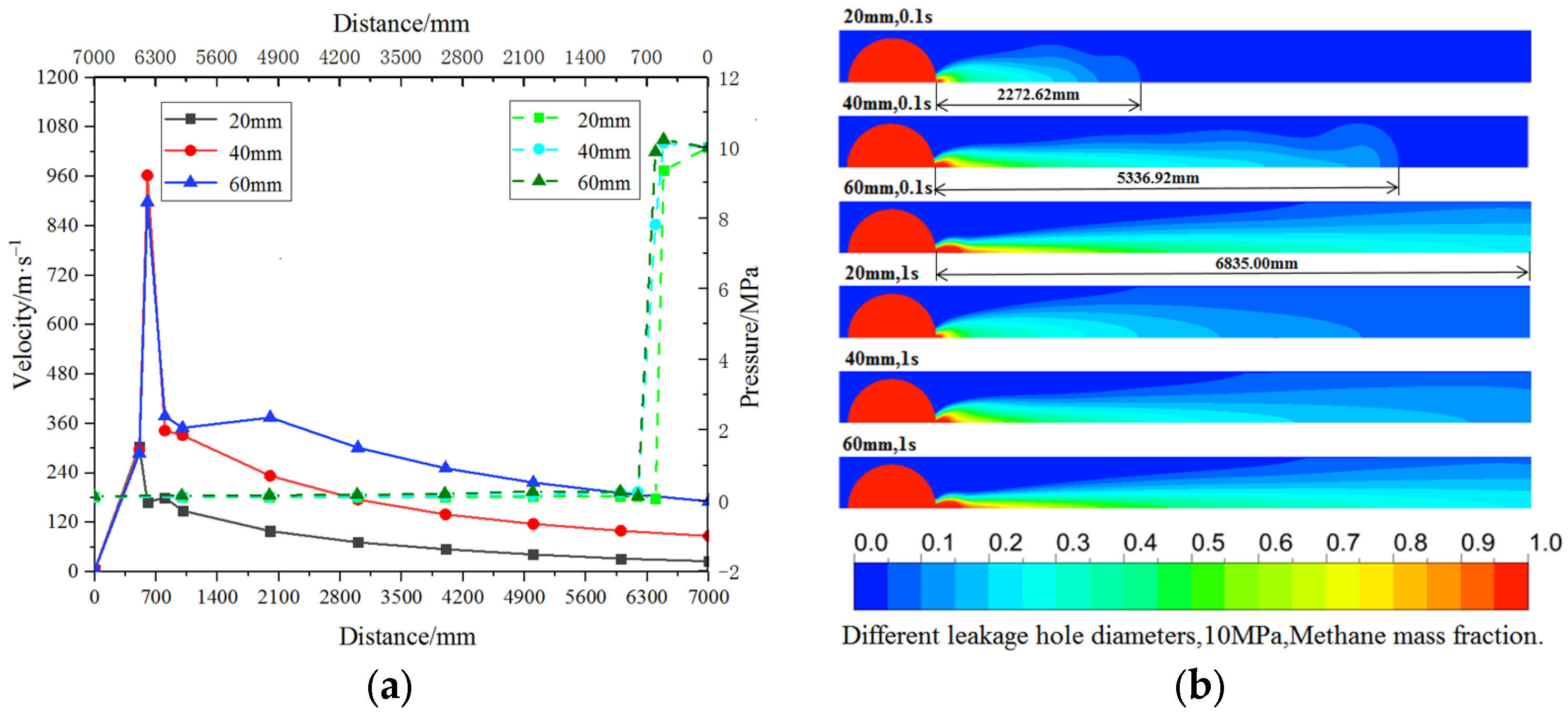
3.1.1. The Influence of Leakage Aperture on the Diffusion of Leakage in High-Pressure Gas Pipeline

The size of the pipe leak hole directly affects the gas leakage diffusion; the leakage diffusion of circular leak holes with leak hole diameters of 20 mm, 40 mm, and 60 mm were simulated, and the calculated methane leakage volume and leak hole center pressure and velocity are shown in

Table 3. Methane leakage level under different leakage apertures.

Leak Hole Diameter (mm)	Simulated Leakage Rate (kg·s−1)	Leak Hole Center Velocity (m·s−1)	Leak Hole Center Pressure (MPa)
20	6.2654	304.71	9.3448
40	22.6718	296.50	10.1317
60	48.5244	287.90	10.2261

. After calculation and stabilization, the leakage pressure-velocity changes at the monitoring points in the vertical direction between the leak holes and the pipeline, and the methane mass distribution cloud diagrams on the cross section of the pipeline are shown in Figure 6.

From the data in Table 3, it can be seen that the simulated leakage volume increases sharply with the increase in leak hole diameter, while the central velocity of the leak hole decreases, and the central velocity of the leak hole decreases by 16.81 m/s when the diameter of the leak hole is increased from 20 mm to 60 mm. From Figure 6a, it can be seen that the trend of velocity change of each monitoring point is the same in different holes, and the velocity is larger near the leak hole, and gradually decreases with the increase in distance. In the side away from the leak hole, the larger the leak hole diameter is, the larger the velocity of the corresponding monitoring point is. At different hole diameters, the maximum value of pressure is near the leak hole, and then decreases sharply with the increase in injection distance; in the calculation domain 800 mm away from the pipe center, the pressure value of each hole diameter is slightly higher than the standard atmospheric pressure, and the pressure of the corresponding monitoring point increases slightly with the increase in hole diameter. Combined with the mass distribution of methane in the pipeline cross-section in Figure 6b, it can be seen that with the increase in leakage aperture, the leakage area of methane gas in the direction of the thickness of the computational domain in the same time is larger, the area of high concentration of methane in the computational domain is larger, and the spray distance is also increased; when the leakage time is 0.1 s, and the leakage aperture diameter is 20 mm, the jet distance is 2272.62 mm; when the leakage aperture is increased to 40 mm, the jet distance is increased to 5336.92 mm; when the leakage aperture is increased to 60 mm, the methane gas is distributed throughout the vertical cross-section.

3.1.2. The Influence of Leak Hole Shape on Leakage Diffusion in High-Pressure Gas Pipeline

Different leak hole shapes affect the ejection state of the leaking gas, which in turn affects the level of gas leakage, so three common pipe leak hole shapes, as shown in Figure 7, were selected for the simulation and analysis of leakage diffusion.

When the area of the leak hole is 3.14 × 10⁻⁴ m² and the delivery pressure is 10 MPa, the leakage levels under the three leak hole shapes are calculated as shown in

Table 4. Leakage level under different leak hole shapes.

Leak Hole Shape	Simulated Leakage Amount (kg·s−1)	Leak Hole Center Velocity (m·s−1)	Leak Hole Center Pressure (MPa)
Circular	6.2654	304.71	9.3448
Rectangular	6.7168	310.28	8.8314
Diamond	6.6988	298.77	9.2245

; after computational stabilization, the leakage velocity–pressure curves of the monitoring points in the perpendicular direction between the leak holes. The pipeline and methane mass distribution maps on the pipeline cross-section are shown in Figure 8.

From the data in Table 4, it can be seen that for different leak hole shapes, the leakage volume is rectangular > diamond > circular; the velocity at the center of the leak hole is rectangular > circular > diamond. As can be seen from Figure 8a, the velocity change trend of each monitoring point under different leak hole shapes is the same and the velocity value of the corresponding monitoring point under each shape is not much different; in the vicinity of the leak hole, the different size and shape of the methane jet core area at different hole diameters resulted in fluctuating values of the leakage velocity at this location; under different leak hole shapes, the pressure values of each monitoring point are not much different, and the rule of change is the same. As can be seen from Figure 8b, the jet shape of the methane jet is different under different leak hole shapes, and the distribution range of methane jet is larger in the vertical cross-section within the same time in the diamond holes, followed by the circular holes; compared with the circular leak holes, the shape distribution of methane leaked from the rectangular and diamond holes is more regular. For the jet distance, when the leakage time is 0.1 s, the jet distance is 2150.87 mm when the shape of the leak hole is diamond; when the shape of the leak hole is circular, the jet distance increases to 2272.62 mm; when the shape of the leak hole is rectangular, the jet distance is farthest at 2581.05 mm.

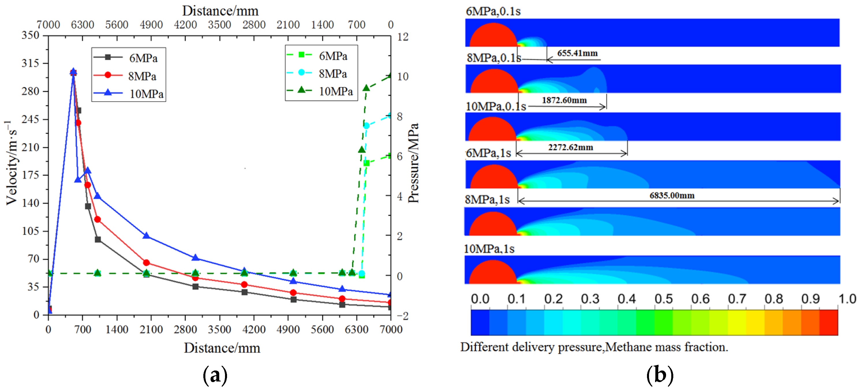
3.1.3. Influence of Delivery Pressure on the Spread of Leaks in High-Pressure Gas Pipelines

In order to investigate the relevant laws of natural gas pipeline leakage under different transmission pressures, between 6 MPa~10 MPa transmission pressure (the leak hole is a circular hole with a diameter of 20 mm), simulation calculations were carried out by taking different transmission pressures. The calculation results are shown in

Table 5. Leakage levels at different delivery pressures.

Delivery Pressure (MPa)	Simulated Leakage Amount (kg·s−1)	Leak Hole Center Velocity (m·s−1)	Leak Hole Center Pressure (MPa)
6	3.8444	303.52	5.6351
8	5.0598	303.93	7.4978
10	6.2654	304.71	9.3448

, and the leakage velocity–pressure change curves of the monitoring points in the vertical direction of the leak holes and pipelines under different transmission pressures and the mass distribution of methane in the pipeline cross-section are shown in Figure 9.

From the data in Table 5, it can be seen that the simulated methane leakage rate gradually increases with the increase in delivery pressure, the pressure at the center of the leak hole increases with the increase in delivery pressure, while the methane leak velocity at the center of the leak hole remains essentially unchanged. Combined with the theoretical formula for the leakage velocity of small holes, it can be seen that the ratio of the leak hole to the diameter of the pipeline is small, ignoring the pressure drop caused by the leakage of the pipeline. When the pressure at the center of the leak hole is higher than the critical pressure, the size of the leakage velocity is related to the ratio of pressure and density, and the ratio of pressure and density of compressible gas at the same temperature is a fixed value. Therefore, after the leakage reaches a steady state, the center velocity of the leak hole is basically the same at all pressures.

As can be seen from Figure 9a, the trend of the velocity change in each monitoring point under different pressures is basically the same; on the side away from the leak hole, the larger the delivery pressure is, the larger the corresponding gas leakage velocity of the monitoring point; when the delivery pressure increases, the pressure value near the leak hole increases; in the calculation domain beyond 800 mm from the center of the pipeline, the change in delivery pressure has little effect on the pressure change at the monitoring point, and the pressure value at each monitoring point is slightly larger than the standard atmospheric pressure. As can be seen from Figure 9b, the larger the delivery pressure, the larger the area of leakage gas spreading in the thickness cross-section of the calculation domain at the same time, the larger the area of high methane concentration in the propagation range, and the shorter the time required for leakage gas to spread to the boundary of the calculation domain; when the leakage time is 0.1 s and the delivery pressure is 6 MPa, the leakage gas jet distance is 655.41 mm, and when the delivery pressure is increased to 8 MPa, the jet distance increases to 1872.41 mm; when the delivery pressure increases to 10 MPa, the farthest jet distance is 2272.62 mm.

3.2. Correction of Pipeline Small Hole Leakage Calculation Based on Numerical Calculation Method

By comparing the error analysis of different calculation methods and experimental pipeline leakage in Section 2.1 and Section 2.2, it can be seen that the error of calculating pipeline leakage using theoretical formulas is larger, and the numerical simulation calculation of pipeline leakage is more accurate, so in order to accurately calculate the leakage of small holes in the gas transmission pipeline, it is necessary to correct the theoretical calculation formula of pipeline leakage from small holes.

3.2.1. Correction of the Influence Coefficient of Pipeline Leakage Pressure

Using the theoretical calculation formula for small hole leakage in Section 2.1, the theoretical leakage under different delivery pressures was calculated for the circular hole with a diameter of 20 mm for the leak hole, and the calculated leakage values are shown in

Table 6. Summary of leakage rate from pipelines of different transport pressures.

Delivery Pressure (MPa)	Simulated Leakage Rate (kg·s−1)	Theoretical Leakage Rate (kg·s−1)	Leakage Difference (kg·s−1)	Relative Error
6	3.8444	3.3454	0.4990	−12.98%
6.5	4.1634	3.6370	0.5264	−12.64%
7	4.4538	3.9314	0.5224	−11.73%
7.5	4.7616	4.2278	0.5338	−11.21%
8	5.0598	4.5258	0.5340	−10.55%
8.5	5.3606	4.8267	0.5339	−9.96%
9	5.6622	5.1291	0.5331	−9.42%
9.5	5.9742	5.4338	0.5404	−9.05%
10	6.2654	5.7390	0.5264	−8.40%

.

As can be seen from the comparative leakage data in Table 6, the theoretically calculated leakage under different delivery pressures is smaller than the simulated leakage. With the increase in delivery pressure, the error between the theoretical leakage and the simulated leakage gradually decreases, and the difference in leakage under each pressure is between 0.49 kg·s⁻¹ and 0.55 kg·s⁻¹, with the overall range of the relative error being between −8.40% and 12.98%.

By analyzing the difference between the theoretical formula and the simulated leakage calculation, the main reasons for this error are discussed:

(1)

The theoretical formula for calculating the leakage rate of the pipeline is only applicable in cases where the gas pressure inside the pipeline is constant during the leakage process, and when the leakage of the pipeline causes the pressure inside the pipeline to change, the calculation accuracy of the model is reduced.

(2)

The theoretical calculation model is based on assumptions, such as that the gas in the pipe is regarded as an incompressible ideal gas, and the gas flow process in the pipe is regarded as an adiabatic flow, which is inconsistent with the leakage process in an actual situation.

As can be seen from Equation (2), when the external ambient temperature, leak hole diameter is the same, the amount of leakage is only related to the pressure in the pipe. Therefore, the introduction of pressure-related correction coefficient α, the corrected theoretical leakage calculation formula is as follows:

$$Q_x=\frac{Q}{\alpha }$$

(5)

Using the leakage data in Table 6 to calculate the correction coefficients under different delivery pressures, the correction coefficients for pressure p_k were obtained by fitting the calculation results based on the least squares method: $\alpha =0.01166p_k+0.8001$. Then, the corrected theoretical calculation formula for the leakage volume of high-pressure gas transmission pipeline is:

$$Q_x=\frac{C_d{p}_k\cdot \frac{\pi d_0^2}{4}\sqrt{\frac{kM}{ZRT}\cdot {\left(\frac{2}{k+1}\right)}^{\frac{k+1}{k-1}}}}{0.01166p_k+0.8001}$$

(6)

Using Equation (6) to calculate the leakage rate under different delivery pressures, the relative errors before and after correction are shown in

Table 7. Summary of relative errors in leakage rate before and after corrections for different delivery pressures.

Leak Hole Shape	Delivery Pressure (MPa)	Simulated Leakage Rate (kg·s−1)	Theoretical Leakage after Pressure Correction.(kg·s−1)	Relative Error before Correction	Relative Error after Correction
Circular	6	3.8444	3.8451	−12.98%	0.02%
	6.5	4.1634	4.1524	−12.64%	−0.26%
	7	4.4538	4.4588	−11.73%	0.11%
	7.5	4.7616	4.7635	−11.21%	0.04%
	8	5.0598	5.0665	−10.55%	0.13%
	8.5	5.3606	5.3677	−9.96%	0.13%
	9	5.6622	5.6673	−9.42%	0.09%
	9.5	5.9742	5.9655	−9.05%	−0.15%
	10	6.2654	6.2616	−8.40%	−0.06%

.

As can be seen from the data in Table 7, the relative error between the leakage calculated by the corrected theoretical formula and the simulated leakage is significantly reduced, with the error range decreasing from −8.40%~−12.98% to between −0.26% and 0.13%.

3.2.2. Correction of the Influence Coefficient of Pipeline Leak Hole Shape

Based on the correction results of circular leak holes under different pressures in Section 3.2.1, the influence of different leak hole shapes on gas leakage flow rate was analyzed. Simulations of rectangular and diamond-shaped holes with the same area under different transport pressures were conducted, and the calculated results are summarized in

Table 8. Summary of leakage rate from pipes with different leak hole shapes.

Leak Hole Shape	Delivery Pressure (MPa)	Simulated Leakage Rate (kg·s−1)	Theoretical Leakage Rate after Pressure Correction (kg·s−1)	Relative Error
Rectangular	6	4.1348	3.8451	−7.01%
	8	5.4134	5.0659	−6.42%
	10	6.7124	6.2605	−6.73%
Diamond	6	4.0882	3.8451	−5.95%
	8	5.3940	5.0659	−6.08%
	10	6.6988	6.2605	−6.54%

.

From the data in Table 8, it can be seen that the error in calculating the leakage of rectangular and diamond-shaped holes using the modified circular hole leakage formula is still large, and the relative error range is between −6.08% and −7.01%. In order to eliminate the influence of the shape of the leak hole, the hole flow coefficient C_d was introduced, calculated to obtain the rectangular and diamond hole correction coefficient of 1.072 and 1.066. The relative errors of leakage from different shaped leak holes before and after correction are shown in

Table 9. Summary of relative errors in leakage rate before and after correction for different leak hole shapes.

Leak Hole Shape	Delivery Pressure (MPa)	Simulated Leakage Rate (kg·s−1)	Theoretical Leakage Rate after Hole Correction (kg·s−1)	Relative Error before Correction	Relative Error after Correction
Rectangular	6	4.1348	4.1219	−7.01%	−0.31%
	8	5.4134	5.4306	−6.42%	0.32%
	10	6.7124	6.7113	−6.73%	−0.02%
Diamond	6	4.0882	4.0988	−5.95%	0.26%
	8	5.3940	5.4002	−6.08%	0.11%
	10	6.6988	6.6737	−6.54%	−0.38%

.

From the data in Table 9, it can be seen that the relative error between the leakage calculated by the theoretical formula and the simulated leakage after the hole correction is significantly reduced, with the error range between −0.38% and 0.32%; the rectangular and diamond-shaped holes have calculated leakage values that are significantly closer to the simulated leakage with higher accuracy after considering the hole flow coefficients.

3.2.3. Correction of the Coefficient of Influence of the Diameter of the Leak Hole of the Pipeline

Based on the correction results for circular leak holes under different pressures in Section 3.2.1, the influence of different leak hole shapes on gas leakage was analyzed, and the leakage of rectangular and diamond leak holes of the same area under different delivery pressures were simulated, respectively. The relative error between theoretical and simulated leakage under different leak hole diameters is shown in

Table 10. Summary of leakage rate from pipes with different leakage apertures.

Leak Hole Diameter (mm)	Delivery Pressure (MPa)	Simulated Leakage Rate (kg·s−1)	Theoretical Leakage Rate after Pressure Correction (kg·s−1)	Relative Error
40	6	13.6930	15.3802	12.32%
	8	18.1847	20.2636	11.43%
	10	22.6718	25.0422	10.46%
60	6	29.3189	34.6055	18.03%
	8	38.9684	45.5931	17.00%
	10	48.5244	56.3449	16.12%

.

From the data in Table 10, it can be seen that when the leakage aperture changes, the relative error range of the leakage volume obtained by using the pressure-corrected leakage volume calculation formula in Section 3.2.1 is between 10.46% and 18.03%. Therefore, the correction coefficient λ, related to the aperture diameter, was introduced in the correction formula, and the corrected theoretical leakage calculation formula is:

$$Q_x=\frac{Q}{\alpha \lambda }$$

(7)

The correction coefficients under different leak hole diameters were calculated using the leakage rate data in Table 10, and the correction coefficients were obtained by fitting the calculation results based on the least squares method to obtain the equation of the correction coefficients with respect to the leak hole diameters d₀: $\lambda =0.00425d_0+0.92475$. Combining the results of the corrections in Section 3.2.1 and Section 3.2.2, the corrected theoretical formula for leakage from small holes in the gas transmission pipeline is derived as follows:

$$Q_x=\frac{C_d{p}_k\cdot \frac{\pi d_0^2}{4}\sqrt{\frac{kM}{ZRT}\cdot {\left(\frac{2}{k+1}\right)}^{\frac{k+1}{k-1}}}}{\left(0.01166p_k+0.8001\right)\cdot \left(0.00425d_0+0.92475\right)}$$

(8)

The conditions under which Equation (8) applies:

①

p_i > p_ic.

②

d₀/D ≤ 0.2 (when leak holes are rectangular or diamond-shaped, calculate equivalent round hole diameter by area.)

③

Select the corresponding hole flow coefficient according to the shape of the leak hole.

④

The formula applies only to the leakage of gas from the pipe into the atmosphere; the leakage of buried pipelines or pipelines under other laying conditions should be analyzed separately.

Using the corrected theoretical formula, the leakage rate under different leak hole diameters was calculated, and the relative errors before and after correction are shown in

Table 11. Summary of relative errors in leakage rate before and after correction for different hole sizes.

Leak Hole Diameter (mm)	Delivery Pressure (MPa)	Simulated Leakage Rate (kg·s−1)	Theoretical Leakage Rate after Aperture Correction (kg·s−1)	Relative Error before Correction	Relative Error after Correction
40	6	13.6930	14.0460	12.32%	2.60%
	8	18.1847	18.5098	11.43%	1.79%
	10	22.6718	22.8748	10.46%	0.90%
60	6	29.3189	29.3329	18.03%	0.05%
	8	38.9684	38.6464	17.00%	−0.83%
	10	48.5244	47.7600	16.12%	−1.58%

.

As can be seen from the data in Table 11, the relative error between the leakage calculated using the aperture-corrected formula and the simulated leakage rate is significantly reduced, with the error range falling from 10.46%~18.03% to between −1.58% and 2.60%.

4. Conclusions

This paper simulates the experimental process of small hole leakage of pipelines under different pressures, analyzes the influence of different influencing factors on the leakage spread of high-pressure pipelines, corrects the theoretical formula of small-hole leakage of pipelines based on the simulated leakage rate, and draws the following conclusions:

(1)

Considering the complex flow process of gas in the pipeline and the influence of the gas interaction between inside and outside the pipeline on the leakage of the pipeline, a three-dimensional leakage diffusion model coupling the pipeline and the air domain was established based on the component transport model and the selection of methane–air mixture components, and the leakage of the experimental pipeline was simulated and analyzed under different influencing factors, which resulted in the relative error range of the experimental leakage and the simulated leakage from −5.03% to −8.65%, which verifies the accuracy of the numerical calculation model of this paper.

(2)

Comparative analysis of the leakage diffusion process of high-pressure pipelines under different influencing factors shows that when the hole diameter increases from 20 mm to 60 mm, the gas leakage velocity at the center of the leak hole decreases by 16.81 m/s, and the leakage volume increases by 42.259 kg/s⁻¹. For leak holes in the same area, the order of leakage is rectangle > diamond > circle; compared with circular leak holes, the shapes of gas leakage velocity distribution of rectangular and diamond leak holes are more regular, and the range of leakage velocity distribution is larger. With the increase in delivery pressure, the amount of gas leakage gradually increases; when the conveying pressure increased from 6 MPa to 10 MPa, the leakage 0.1 s gas injection distance increased by 1617.21 mm.

(3)

Using the least squares method to linearly fit the error between the simulated leakage and the theoretical leakage, the correction coefficients for the delivery pressure, the shape of the leak hole, and the diameter of the leak hole were solved, and the corrected leakage formula was obtained. The theoretical leakage calculated by the corrected formula was closer to the simulated leakage, and the relative error range between the two was reduced from −8.40%~18.03% before correction to −1.58%~2.60%, which significantly improves accuracy.

Based on the numerical calculation method, this paper proposed a correction method for the calculation of pipeline small-hole leakage under the overhead scenario, which provides data support for the quantitative risk evaluation of natural gas pipelines. The correction results will be further verified using relevant experimental tests in the future. Since the leakage involved in this paper is small-hole leakage, the pressure change in the pipeline is small at this time, which can be approximated as steady-state leakage. When the leakage hole diameter is larger or the pipe is broken, the cutoff valve of the pipe is closed, and the pressure in the pipe gradually decreases with the leakage. This kind of dynamic leakage process of the pipe is the key direction of the next research, and at the same time, the leakage diffusion of the pipeline under different laying conditions will be explored to supplement and improve the correction results.

References

1. Hou, Z.M.; Luo, J.S.; Cao, C.; Ding, G.S. Development and contribution of natural gas industry under China’s carbon neutrality target. Eng. Sci. Technol. 2023, 55, 243–252. (In Chinese) [Google Scholar]
2. Li, J.; She, Y.G.; Gao, Y.; Li, M.P.; Yang, G.I.; Shi, Y.J. Natural gas industry in China: Development situation and prospect. Nat. Gas. Ind. 2020, 7, 604–613. [Google Scholar] [CrossRef]
3. Zhu, Z.; Liao, Q.; Qiu, R.; Liang, Y.T.; Song, Y.; Xue, S. Technical and economic analysis of long-distance hydrogen pipeline transportation. Petrol. Sci. Bull. 2023, 1, 112–124. (In Chinese) [Google Scholar]
4. He, D.B.; Jia, C.G.; Wei, Y.S.; Guo, J.L.; Ji, G.; Li, Y.L. World natural gas industry situation and development trend. Nat. Gas. Ind. 2022, 42, 1–12. (In Chinese) [Google Scholar]
5. Ding, Y.Q.; Zhou, H.Y.; Lu, Y.; Cheng, J.H.; Ye, B.T.; Li, W.W.; Ma, Q.R. Study on the influence of dynamic response of buried pipeline explosion based on multiphase coupling. Chem. Mach. 2019, 46, 425–432. (In Chinese) [Google Scholar]
6. Levenspiel, O. Engineering Flow and Heat Exchange; Plenum Press: New York, NY, USA, 1984. [Google Scholar]
7. Crowl, D.A. Chemical Process Safety: Fundamentals with Application; Prentice-Hall: Upper Saddle River, NJ, USA, 1990. [Google Scholar]
8. Woodward, J.L.; Mudan, K.S. Liquid and gas discharge rates through holes in process vessels. J. Loss Prev. Process Ind. 1991, 4, 161–165. [Google Scholar] [CrossRef]
9. Montiel, H.; Vilchez, J.A.; Casal, J.; Arnaldos, J. Mathematical modeling of accidental gas release. J. Hazard. Mater. 1998, 59, 211–233. [Google Scholar] [CrossRef]
10. Xiang, S.P.; Feng, L.; Zhou, Y.C. Leakage model of natural gas pipeline. Nat. Gas. Ind. 2007, 27, 100–102. (In Chinese) [Google Scholar]
11. Wang, Z.Q.; Feng, W.X.; Li, Z.R.; Xiang, X.Q.; Li, B.J.; Cheng, W.Y. High Pressure Gas Pipeline Leakage Model. Oil Gas. Storage Transp. 2009, 28, 28–30. (In Chinese) [Google Scholar]
12. Zhang, P.; Zhou, L.; Lu, C.; He, L.; Wang, X.L.; Zhao, H. GERG-2008 equation was used to calculate natural gas compression factor and hydrocarbon dew point. Nat. Gas. Ind. 2021, 41, 134–143. (In Chinese) [Google Scholar]
13. Chen, Q.; Xing, X.K.; Jin, C.; Zuo, L.L.; Wu, J.H.; Wang, W.S. A novel method for transient leakage flow rate calculation of gas transmission pipelines. J. Nat. Gas. Sci. Eng. 2022, 77, 103261. [Google Scholar] [CrossRef]
14. Hou, Q.M.; Yang, D.H.; Li, X.Y.; Xiao, G.H.; Ho, S.C.M. Modified Leakage Rate Calculation Models of Natural Gas Pipelines. Math. Probl. Eng. 2020, 2020, 6673107. [Google Scholar] [CrossRef]
15. Sun, J.F. Research on Natural Gas Pipeline Leakage Process Simulation and Leakage Calculation. Master’s Thesis, China University of Petroleum, Beijing, China, 2020; pp. 15–20. (In Chinese). [Google Scholar]
16. Hu, H.B. Analysis of the current situation of natural gas pipeline leakage research. Contemp. Chem. Ind. 2016, 45, 352–354. (In Chinese) [Google Scholar]
17. Tauseef, S.M.; Rashtchian, D.; Abbasi, S.A. CFD-based simulation of dense gas dispersion in presence of obstacles. J. Loss Prev. Process Ind. 2011, 24, 371–376. [Google Scholar] [CrossRef]
18. Ma, J.; Liu, H.S.; Liu, L.; Xie, M. Simulation study on the cryogenic liquid nitrogen jets: Effects of equations of state and turbulence models. Cryogenics 2021, 117, 103330. [Google Scholar] [CrossRef]
19. Amir, E.M.; Mahmood, F.J.; Ahmad, A.; Ali, J.M. CFD analysis of natural gas emission from damaged pipelines: Correlation development for leakage estimation. J. Clean. Prod. 2018, 199, 257–271. [Google Scholar]
20. Gao, B.; Zhao, R.T.; Kuai, C.T.; Hu, M.Y.; Wang, G.F. Numerical simulation study on leakage diffusion and failure consequences of high pressure hydrogen-doped natural gas pipeline. J. Liaoning. Univ. Petrochem. Technol. 2023, 43, 60–67. (In Chinese) [Google Scholar]
21. Liu, C.W.; Liao, Y.H.; Liang, J.; Cui, Z.X.; Li, Y.X. Quantifying methane release and dispersion estimations for buried natural gas pipeline leakages. Process. Saf. Environ. Prot. 2021, 146, 552–563. [Google Scholar] [CrossRef]
22. Javad, B.; Esmaeil, F.; Ali, R. CFD investigation of natural gas leakage and propagation from buried pipeline for anisotropic and partially saturated multilayer soil. J. Clean. Prod. 2020, 277, 123940. [Google Scholar]
23. Li, X.H.; Chen, G.M.; Zhang, R.Z.; Zhu, H.W.; Fu, J.M. Simulation and assessment of underwater gas release and dispersion from subsea gas pipelines leak. Process. Saf. Environ. Prot. 2018, 119, 46–57. [Google Scholar]
24. Shi, Y.D.; Ge, T.M.; Zhang, Z.F. Study on gas leakage and diffusion simulation and influencing factors of submarine gas pipeline. Chem. Eng. Oil Gas. 2020, 49, 109–115. (In Chinese) [Google Scholar]
25. Duan, C.G. Gas Transmission and Distribution; China Construction Industry Press: Beijing, China, 2001. (In Chinese) [Google Scholar]
26. Cong, Z.W.; Ma, T.X.; Yu, D.L.; Wu, D.R. Characterization of natural gas pipeline leak diffusion in foothill terrain. J. Saf. Environ. 2022, 22, 2078–2085. (In Chinese) [Google Scholar]
27. Wang, C.P. Study on Leakage Simulation and Risk Control Measures of Long-Distance Natural Gas Pipeline. Master’s Thesis, China University of Petroleum, Beijing, China, 2014; pp. 17–19. (In Chinese). [Google Scholar]
28. Teng, Z.C. Finite Element Simulation of Saint-Venant’s Principle. Value Eng. 2018, 37, 188–190. (In Chinese) [Google Scholar]
Figure 1. Schematic diagram of gas pipeline leakage.
Energies 16 07255 g001
Figure 2. (a) Numerical simulation diagram of global coupling in experimental pipelines; (b) partial enlarged view of experimental pipeline.
Energies 16 07255 g002
Figure 3. (a) Cloud map of velocity distribution inside the experimental pipeline; (b) comparison curve of pipeline leakage rate under different conditions.
Energies 16 07255 g003
Figure 4. Schematic diagram of leakage diffusion model for high-pressure gas pipeline.
Energies 16 07255 g004
Figure 5. (a) Cloud map of methane leakage velocity distribution; (b) cloud map of methane mass fraction distribution.
Energies 16 07255 g005
Figure 6. (a) Velocity–pressure variation curve under different apertures; (b) cloud map of methane mass fraction distribution.
Energies 16 07255 g006
Figure 7. Schematic diagram of pipe leak hole shape.
Energies 16 07255 g007
Figure 8. (a) Velocity–pressure variation curve under different leak hole shapes; (b) cloud map of methane mass fraction distribution.
Energies 16 07255 g008
Figure 9. (a) Velocity–pressure variation curve under different delivery pressures; (b) cloud map of methane mass fraction distribution.
Energies 16 07255 g009