Optimizing Instrument Transformer Performance through Adaptive Blind Equalization and Genetic Algorithms

Abstract

In real-world scenarios, deviations in the frequency response of instrumentation transformers can lead to distorted harmonic measurements, highlighting the critical role harmonic measurement plays in assessing power quality. The blind channel equalization technique offers a potential solution to improve the frequency response of a large number of instrumentation transformers already installed in substations. These transformers were designed to accurately measure only the fundamental phasor component. Therefore, in order to use them for harmonic phasor measurement, methodologies for reducing frequency distortion must be applied. In this work, we propose a novel approach to improve the frequency response of the instrument transformer using adaptive blind equalization. The blind technique can compensate for distortions caused by voltage and current transducers without requiring prior knowledge of input signals or circuit characteristics. The proposed methodology uses a Linear Prediction Filter to convert the colored noise present at the channel output into white noise. Furthermore, a genetic algorithm is used to find a pole to cancel possible zeroes present in the frequency response of some transducers. The main advantage of blind equalization with the genetic algorithm is its independence, operating without clear information about the channel or the input signal. Through extensive experimentation, we demonstrate the effectiveness of the proposed methodology in significantly reducing the absolute error in ratio and phase caused by current and voltage transformers. Simulated and laboratory experiments are presented in this paper.

1. Introduction

Accurate estimation of harmonic components has become essential for assessing Power Quality (PQ), as the insertion of harmonic distortion into Electric Power Systems (EPS) has grown significantly [1]. This increase is the result of the growing presence of nonlinear loads and renewable energy sources in EPS. These combined factors contribute to the deterioration of PQ, resulting in issues such as voltage drops, excessive heating, and malfunctioning of sensitive devices [2]. Therefore, the identification and effective mitigation of harmonic components are crucial to ensure the reliability and proper performance of modern grids [3,4].

Monitoring current and voltage harmonics is essential for analyzing their propagation in the network and identifying critical situations. To improve the PQ, it is important to carry out large-scale harmonic measurements and it is also possible to use advanced signal processing techniques that allow the identification of users responsible for harmonic pollution, making it possible to plan actions for the mitigation of the harmonic state of the network [5]. To access the harmonic distortion at the high voltage (HV) and medium voltage (MV) primary side, the Instrument Transformers (IT) play a crucial role. The accuracy of these transformers is essential to ensure the precision of harmonic measurements and, consequently, the reliability of PQ analyses [6]. Nevertheless, the majority of installed IT have accuracy classes suitable only for the fundamental frequency [7]. This limitation can result in substantial distortions in the secondary signal, since the frequency response of these IT is not constant within the frequency range of interest [8].

Numerous methods have been presented in the literature to correct errors introduced by Instrument Transformers (IT) in non-fundamental components. A significant proportion of these techniques requires laboratory calibration, which involves measuring the frequency response of the transducer [9,10,11]. This approach entails measuring the transformer’s response under different operating conditions and determining the necessary corrections. Nonetheless, it is crucial to bear in mind that the adjustments achieved in the lab may not be wholly applicable in real-world field conditions, as diverse environmental and operational variables come into play. Factors like applied loads, ambient temperature, and other external influences can affect the transformer’s performance in distinct ways compared to a controlled laboratory setting [12,13,14,15,16,17].

Another widely used technique is the utilization of post-compensation filters, which can be digital filters such as Finite Impulse Response (FIR), Infinite Impulse Response (IIR), or Fourier Filters [18,19,20,21,22]. Their implementation is straightforward, involving finding the inverse function of the transducer. However, this methodology requires the identification of the transducer’s transfer function, which is typically conducted in a laboratory setting, thereby extending the limitations of load and temperature effects. Additionally, the obtained system may be unstable, which can hinder proper implementation.

Other methods in the literature take into account the nonlinear characteristics of transducers, which not only introduce new harmonics on the secondary side, even if the primary signal is undistorted, but also amplify those already present in the primary side signal. Although this is a significant problem currently being researched in the literature [23,24,25,26,27,28], there is still a substantial gap to be investigated, considering only frequency distortions caused by the purely linear model, as is the case in the research presented in this article.

In [29], a technique called non-blind equalization was proposed to correct frequency distortion caused by transducers. This approach involves adaptively determining the inverse filter, typically a FIR filter, to be used in conjunction with the channel. By utilizing adaptive filtering algorithms such as Recursive Least-Squares (RLS) and Least-Mean-Squares (LMS), the equalization process is performed online, resulting in a FIR that behaves as an inverse filter. This implies that if temperature or load variations affect the frequency response, the method will automatically seek to correct this issue. However, the non-blind equalization method requires knowledge of the signal on the primary side of the transformer, which may be accessed by the installation of a Reference Transducer (RT) with a suitable frequency response. This requirement adds complexity to the equalization process due to the need for installing and maintaining the RT.

To overcome the mentioned problem, this work proposes a methodology called blind equalization. This approach is innovative in enhancing transducer performance, as it eliminates the need to have knowledge about the signal on the primary side of the transducer. Unlike traditional methods, this blind equalization technique does not require a reference transducer to generate the training signal for the equalizer. Instead, it employs a forward Linear Prediction Error (LPE) filter, also known as a whitening filter, for transducer equalization. By assuming the presence of white noise with a Gaussian distribution on the primary side of the IT, the method separates the signal component (fundamental plus harmonics) from the noise component on the secondary side of the transducer. The adaptive predictive filter is designed to “whiten” the noise, effectively equalizing the transducer by compensating for the coloring effect caused by the IT on the white noise.

The limitation of the above methodology occurs in case the IT transfer function presents zeros close to the unit circle. In this case, a pole must be included in the equalizer to cancel the zero. However, the FIR filter is not able to include poles. To address this issue, it was necessary to forcibly introduce a pole. The Genetic Algorithm (GA) was employed to autonomously find this pole and stabilize the system for an equalization purpose.

The methodology was tested using simulation and laboratory testing. In the simulation, test transducers whose transfer functions were known beforehand were used. Following this simulation phase, a laboratory experiment was conducted to assess the method’s performance using a real transducer. The results obtained in this study were extremely promising, demonstrating the feasibility of the developed research. It is crucial to emphasize that this paper exclusively addresses the linear characteristics of IT. Consequently, we do not take into account the nonlinear effects resulting from core saturation.

The rest of this paper is organized as follows. An overview of applied techniques are described in Section 2. Section 3 presents the proposed methodology of this work. Section 4 presents the application and results obtained. The conclusion is presented in Section 5.

2. Overview of Applied Techniques

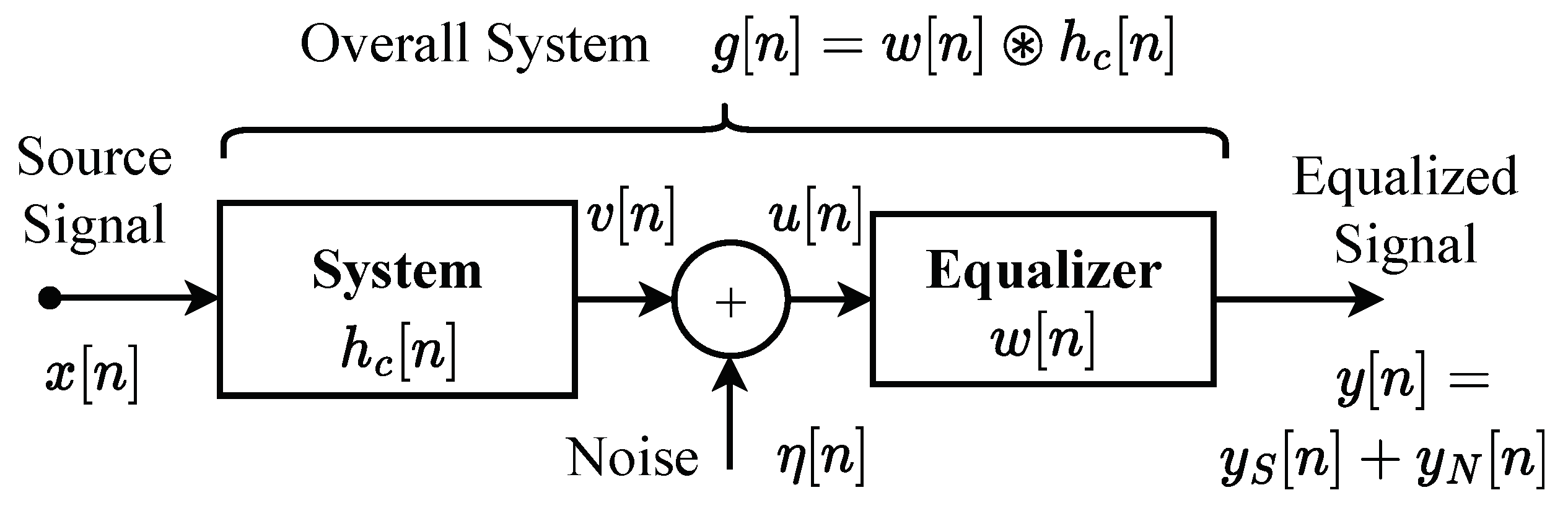
2.1. Blind Equalization

For the processing of adaptive equalization, the communication channel, while processing the received signal, seeks to obtain the inverse impulse response of the channel. In the supervised equalizers or non-blind equalizers [30], the information from the primary side of the channel (transducer) must be known.

The equalizers referred to as non-supervised or blind do not need access to the signal at the channel input in order to perform equalization. Instead of using the signal itself, they rely on statistical information, such as second-order (SOS) or higher-order (HOS) statistics, to achieve the equalization process.

Consider the system shown in Figure 1. Suppose that $x\left[n\right]$ represents the input signal that passes through a Single Input Single Output (SISO) Linear Time Invariant (LTI) system $h_c\left[n\right]$, $v\left[n\right]$ denotes the noise-free signal at the channel output, and $\eta \left[n\right]$ represents the additive noise accounting for measurement noise as well as unexplained physical effects on $v\left[n\right]$. Blind equalization of the $h_c\left[n\right]$ system is a signal processing procedure that aims to restore the original signal $x\left[n\right]$ using only the data $u\left[n\right]$ and certain statistical information about the original signal $x\left[n\right]$.

Continuing with Figure 1, the problem of blind SISO equalization aims to design a filter with an impulse response given by $w\left[n\right]$, utilizing certain assumed characteristics of $x\left[n\right]$, in order to obtain the output of the equalizer $y\left[n\right]$, in which $y_S\left[n\right]$ corresponds to the signal component, and $y_N\left[n\right]$ corresponds to the measurement noise component. The objective is to make $y\left[n\right]$ approximate $x\left[n\right]$ as closely as possible, and the filter $w\left[n\right]$ is referred to as the blind equalizer.

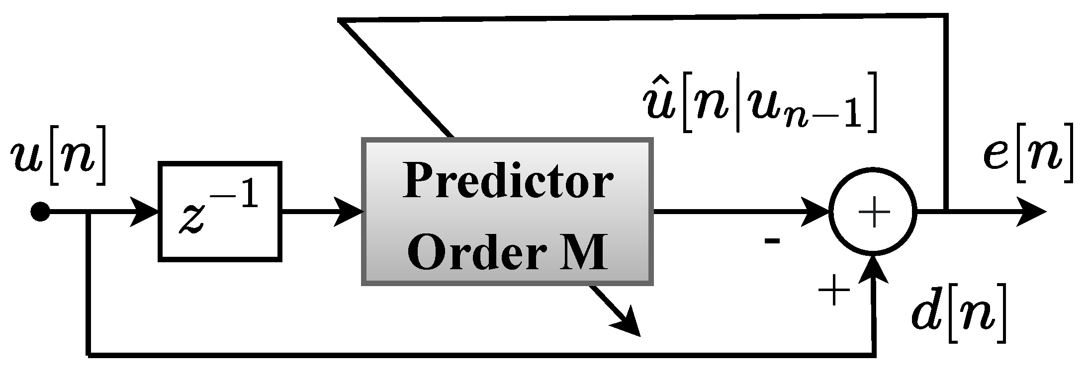
2.2. Linear Prediction Error (LPE) Filter

An approach to blind equalization, relying on second-order statistics (SOS), involves the utilization of LPE filters. The forward LPE filter will be used, in this work, for blind equalization. The forward LPE filter utilizes a prediction procedure to adjust the relevant parameters to minimize the error. Additionally, the LPE filter is also known as a whitening filter, capable of transforming colored noise into white noise.

Figure 2 illustrates the block diagram of a forward LPE filter, which processes the signal to estimate the “present” sample $u\left(n\right)$ by linearly combining the “past” samples ${\mathbf{u}}_{n-1}={[u[n-1],u[n-2],\cdots ,u[n-M]]}^t$, where M represents the order of the filter. The output of the filter, named $\widehat{u}\left[n\right|{\mathbf{u}}_{n-1}]$, is the estimate for $d\left[n\right]=u\left[n\right]$. Then, the error signal $e\left[n\right]$ is minimized, using some statistical criterion, in order to obtain an optimum predictor filter.

To perform blind equalization using the LPE filter, the objective is to design an optimal filter that minimizes the error in terms of Mean Squared Error (MSE). For this, certain assumptions need to be made [30]:

• The SISO LTI system represented by $h_c\left[n\right]$ must be stable and have a minimum phase.
• The source signal $x\left[n\right]$ is a Wide Sense Stationary (WSS) white process with a variance of ${\sigma }_x^2$.
• The noise $\eta \left[n\right]$ is a zero-mean WSS white process with a variance of ${\sigma }_{\eta }^2$.
• The source signal $x\left[n\right]$ is statistically independent of the noise $\eta \left[n\right]$.

In the context of equalizing instrumentation transformers, where access to the primary signal is not available, it becomes possible to equalize the transducer using only the noise signal at its output. In this scenario, the output noise will exhibit coloration due to the propagation of white noise through the channel. Consequently, the predictor filter, by “whitening” the noise, estimates the inverse response of the channel and performs equalization accordingly.

2.3. Genetic Algorithm

Genetic Algorithms (GA) are known as function optimization algorithms, based on Charles Darwin’s theory of evolution and operating on principles similar to the mechanisms of species evolution through genetic combination and alteration [31]. They were introduced by Holland [32] and popularized by Goldberg [33], offering a simplified approach to formulating and solving complex problems with multiple variables [34].

The objective of GA is to choose the most adapted individuals in the population, considering all their characteristics, to achieve the best possible combinations. Although the evolutionary process of the algorithm is random, it follows a determined selection structure based on the adaptation of the individuals [34].

The flowchart of Figure 3 illustrates the adopted scheme in this work for the operation of the GA. The algorithm starts by generating an initial random population of individuals, representing potential solutions to the problem, and then proceeds through several generations. In each iteration of the algorithm, the population generation is updated, and the fitness function, or objective function, is evaluated to assess the individuals’ performance.

The objective function used in this work was the Mean Absolute Error (MAE) of the RLS and LMS algorithms for both simulated and real cases. This error represents the difference between the output of the algorithms RLS and LMS and the desired output (reference) for each iteration. Therefore, the pole value that results in the lowest mean absolute error will be chosen as the individual to be used in the Pre-Filter function ($H_p$). The objective function will be further explained in Section 3.

The individuals will be modified through genetic operators, where the operations of crossover, mutation, evaluation, fitness calculation, selection, and elitism are performed in sequence. A new population with the same number of individuals is generated for the next iteration (generation).

In the stage known as crossover, the population is divided into two parts. Individuals are generated by crossing pairs of parents randomly. For each formed pair of parents, it is determined with a probability of 0.5 whether a crossover process will occur or not. When crossover occurs, a new individual, represented as $x_g$, is generated from the parents, $x_1$ and $x_2$, using a weighted combination controlled by the parameter $\alpha$. The formula expressing this combination is $x_g=\alpha x_1+(1-\alpha )x_2$, with $\alpha$ varying in the range of $(-0.1$ to $1.1)$. The parameter $\alpha$ plays a crucial role in determining the relative influence of each parent on the offspring, allowing the creation of new individuals that inherit characteristics from both parents. The algorithm continues to generate new individuals until the desired population size is reached, preserving genetic diversity while optimizing fitness.

The mutation determines whether the individual will undergo mutation or not, with a probability of 0.02. If a mutation occurs, a vector $\delta$ is added to the individual x, where ${\delta }_i=0.05{\beta }_i{\left(x_R\right)}_i$. Here, ${\beta }_i$ is a random number with a Gaussian distribution, mean zero, and variance one, and $x_R$ is the vector of differences between the maximum and minimum values of the parameters $x_R=(x_U-x_L)$.

In the evaluation step, each individual is assessed in the objective function, where each individual (pole) has a mean error value. This step is detailed in Section 3. The objective function is then incorporated into the fitness function, as proposed in [33], yielding a fitness value for each individual. A value of $\gamma =1.8$ was adopted.

Subsequently, a selection of N individuals among the existing individuals is performed, and each individual can be selected more than once. The probability of an individual being selected each time is equal to the fraction of its fitness value relative to the sum of fitness values of all individuals. In this work, the selection criterion by a roulette wheel was used. The process involves calculating the selection probabilities based on the fitness values of each individual and then selecting the individuals with higher probabilities. In this work, $20\%$ of the best individuals are selected. If the best individual has not been selected for the new population, it is added to the population, and a random individual is excluded. This operation is called elitism.

Finally, it is necessary to employ a stopping criterion. Some options for the stopping criterion can be based on the maximum number of generations, the processing time limit, or the stabilization of the objective function value. In this work, the stopping criterion chosen is the stabilization of the objective function, considering the stabilization when the objective function varies less than 0.1% of its value in the last five iterations.

3. Proposed Methodology

The present study proposes an innovative approach by combining adaptive blind equalization with the Genetic Algorithm (GA) to equalize Voltage Transformers (VT) and Current Transformers (CT). This strategy has been under explored in the literature but shows great promise. To apply the discussed blind equalization theory and correct the frequency response of VT and CT, where the GA finds the value of the pole, specific considerations and manipulations were required, some of which are presented in Section 2.2.

The objective function is shown in Figure 4. This block diagram represents the proposed blind equalization scheme. The block $H_c\left(s\right)$ represents the transfer function of the channel (transducer) to be equalized. All blocks within the gray rectangle are in the discrete-time domain, so the transducer’s output signal, $z\left(t\right)$, must be discretized by an analog-to-digital converter. The signal on the High Voltage (HV) or Medium Voltage (MV) side consists of the fundamental component $f\left(t\right)$ distorted by harmonics $h\left(t\right)$ and corrupted by Additive White Gaussian Noise (AWGN) $x\left(t\right)$, or

$$s\left(t\right)=f\left(t\right)+h\left(t\right)+x\left(t\right)$$

(1)

The signal defined by Equation (1) does not satisfy the second assumption presented in Section 2.2. Therefore, the first step is to filter the fundamental and harmonic components of the input signal to isolate only the output noise. This filtering process is performed in the frequency domain by the “FFT Estimator” block, which generates the discrete colored version of the white noise $x\left(t\right)$. In Figure 4, this colored noise is denoted as $u_v\left[n\right]$. The colored noise will later be “whitened” using the predictor filter.

Before the whitening process, the colored noise passes through a pre-filter block $H_p\left(z\right)$, whose purpose is to find the suitable pole value for equalization. The pre-filter block is included if the frequency response of the real transducer has a null response, meaning it has zeros close to the unit circle in the z-plane. This is because equalization using an FIR filter cannot generate poles and, therefore, cannot cancel zeros. The inclusion of the pre-filter is justified as the Genetic Algorithm (GA) can search for the optimal pole value, thereby improving equalization performance. Additionally, it is essential to remember that blind equalization using a predictor filter requires the system under equalization to be stable and have minimum phase, i.e., with poles and zeros inside the unit circle [30].

Next, $u\left[n\right]$ will be the input signal for the predictor filter, and the desired signal $d\left[n\right]$, where the signal will be delayed by a previous sample $u_d\left[n\right]$, and will be equalized by the FIR filter. The adaptive algorithms RLS and LMS will be used to estimate the system coefficients. Finally, the objective function will have the value of the mean error $mean\left(e\right[n\left]\right)$, which represents the difference between the desired signal $d\left[n\right]$ and the equalized output $y\left[n\right]$. This implies that various pole values are tested in $H_p$, and the smaller the error value, the more suitable the pole value is for the system.

4. Discussion and Results

The results for blind equalization with GA applied to a VT using the LPE filter and employing RLS and LMS algorithms cover two distinct scenarios. Firstly, the focus was on the simulated system, where this scenario involved a theoretical computer-based setup, and a simulated RLC model was used to represent the transformer. Additionally, we employed the Monte Carlo method for statistical analysis, conducting a total of 100 experiments. In a second phase, adaptive blind equalization tests were conducted using a real system. The statistical treatment of real system cases involved segmenting the signal to obtain average coefficients, aiming to minimize the error and reduce estimation noise.

In the signal used with the fundamental frequency of 50 Hz, the following harmonics were added: $5,13,21,40,$ and 45, which will consequently be analyzed. The evaluation of results will adhere to the guidelines of the IEC 61869-1 [35] and IEC/TR 61869-103 [36] standards, which defines precision limits for ratio and phase errors of instrument transformers. According to these standards, the allowable range for ratio error is 5%, and the phase error should be within 5 degrees (90 mrad) from the third to the 50th harmonic.

The percentage ratio error and phase error displacement are given, respectively, by:

$$\mathrm{Ratio}\mathrm{Error}(\%)=\left|\frac{\left|\mathrm{Ideal}\mathrm{Ratio}\left(\mathrm{h}\right)-\mathrm{Equalized}\mathrm{Ratio}\left(\mathrm{h}\right)\right|}{\mathrm{Ideal}\mathrm{Ratio}\left(\mathrm{h}\right)}\right|\times 100\%$$

(2)

$$\mathrm{Phase}\mathrm{Error}\left(\mathrm{degrees}\right)=\left|\frac{\left|\mathrm{Ideal}\mathrm{Phase}\left(\mathrm{h}\right)-\mathrm{Equalized}\mathrm{Phase}\left(\mathrm{h}\right)\right|}{\pi }\right|\times 180$$

(3)

where (h) is the harmonic.

All simulations were conducted using Matlab^®, with a sample rate of 128 samples per cycle, corresponding to a sampling frequency of 6400 Hz (128 × 50). For all cases, three signal-to-noise ratio (SNR) levels were tested: 30 dB, 40 dB, and 50 dB, and all 40 dB cases will be illustrated. In all cases, a signal containing the fundamental component and 2% of harmonics of order 5, 13, 21, 40, and 45, corrupted by AWGN, was used. The details of each case are provided below.

4.1. Synthetic Experiments

The RLC model of the transformer used for the first six cases, corresponding to the synthetic experiments, is shown in Figure 5. This model can provide a good approximation of the frequency response of a real transformer, even without considering nonlinear behaviors. In Figure 6, you can observe the frequency response of the transformer (black) and also the results of the RLS algorithm (red) and LMS algorithm (blue), which belong to Case 2. An improvement in the frequency response can be observed due to the proposed method.

Cases 1, 2, and 3 show the results for ratio and phase errors, presented with the empirically inserted pole value $0.133\pm 0.981i$. This value was determined through the pole-zero diagram, Figure 7, where the poles for all cases are illustrated. Additionally, it is noticeable in Figure 7 that there is a pair of zeros outside the unit circle at $0.133\pm 1i$ (red circle), indicating that this transformer model is not minimum-phase. The purpose of the GA is to find a pole to cancel this zero, used in the Pre-Filter ($H_p$) block, but this pole must be inside the unit circle, thus characterizing a stable minimum-phase system, and thus satisfying the first condition for blind equalization in Section 2.2. The zero shown in the Pole-Zero Diagram, Figure 7 can also be observed in Figure 6, where the model has a zero in the frequency response near 1.5 kHz, as well as a resonance near 1.13 kHz.

Figure 7 displays the poles found by the GA for all cases, including the real experiment. As the algorithm found a zero value for the real experiment, it is likely that this transformer is a stable minimum-phase system. However, it is important to note that the transformer’s characteristics are unknown to confirm this assertion. Furthermore, it is evident that the poles found by the GA for the simulated cases are very close to the value that needs to be canceled, indicating that the GA is operating coherently.

The absolute ratio and phase errors for Case 2, with an SNR of 40 dB, are shown in Figure 8a,b. The maximum error for RLS stayed below 1.5%, while for LMS it stayed below 1% for all harmonics. In contrast, for example, for the 21st harmonic, the error reached 250% without equalization. For the phase, both RLS and LMS values stayed below 3 degrees, whereas without equalization, the values approached 14 degrees.

Cases 4, 5, and 6 show the results with the pole value found by the GA, where for Case 4: $0.1442+0.9672i$, Case 5: $0.1384+0.9703i$, and Case 6: $0.1362+0.9569i$, with these values depicted in Figure 7. Case 5 will be illustrated with an SNR of 40 dB in Figure 9a,b. The results of Case 5 indicate that the maximum error for the ratio stayed below $3.9\%$, while the maximum error for phase stayed below 4 degrees. These results are for the 21st harmonic, where without equalization, the error could reach $250\%$ and 14 degrees.

It is important to note that in all six simulated cases, the equalization results were effective in reducing both ratio and phase errors, aligning them with the criteria set by the IEC 61869-1 and IEC/TR 61869-103 standards [35,36].

4.2. Real Experimental

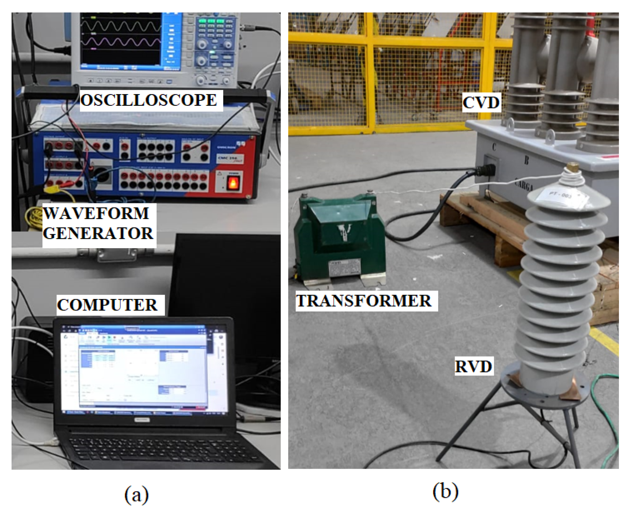
4.2.1. Laboratory Implementation

For the tests conducted under real conditions, a configuration was set up in the laboratory environment. The block diagram representation of the equipment under the test can be observed in Figure 10. In this setup, an arbitrary waveform generator was used to create a sinusoidal signal with Additive White Gaussian Noise (AWGN). This signal is introduced into the secondary winding of a voltage transformer, with its primary winding connected to a Resistive Voltage Divider (RVD) in parallel with a Capacitive Voltage Divider (CVD). The RVD acts as the reference transducer for the sake of comparison results. Since one has access to both the input (waveform generator) and the output (resistive divider), the equalization may be performed in two ways: (i) with the switch open, the step-up transformer equalization is performed; with the switch closed, the equalization of the whole system is performed. To save space, in this article, we presented only the results for equalizing the entire system. The test conducted, although limited, serves as the initial experimental validation of the methodology. Therefore, the frequency distortion considered in the experiment includes the distortion from both the step-up transformer and the capacitive divider.

Figure 11a provides an overview of the processing and acquisition systems. At the heart of this setup is the arbitrary waveform generator, the data acquisition system consisting of an oscilloscope, and the data processing system encompassing a notebook where the equalization algorithm is executed. The representation in Figure 11b highlights the experimental setup, where three devices are visible: the voltage step-up transformer, RVD, and CVD. The step-up transformer is an instrumentation transformer with class 0.3% P75, and turns ration 1:70. The resistive divider is 1000:1. The point A was used as input and B and C as output.

4.2.2. Results for Real Experimental

This section presents results from real cases involving blind equalization (Cases 7, 8, and 9). For these cases, the GA found a pole value equal to “0”, as illustrated in Figure 7. Comprehensive results are presented in

Table 1. Results for Absolute Ratio Error of the harmonic indices of the cases discussed.

Spectrum			Absolute Ratio Error (%)
Harmonic Index			1	5	13	21	40	45
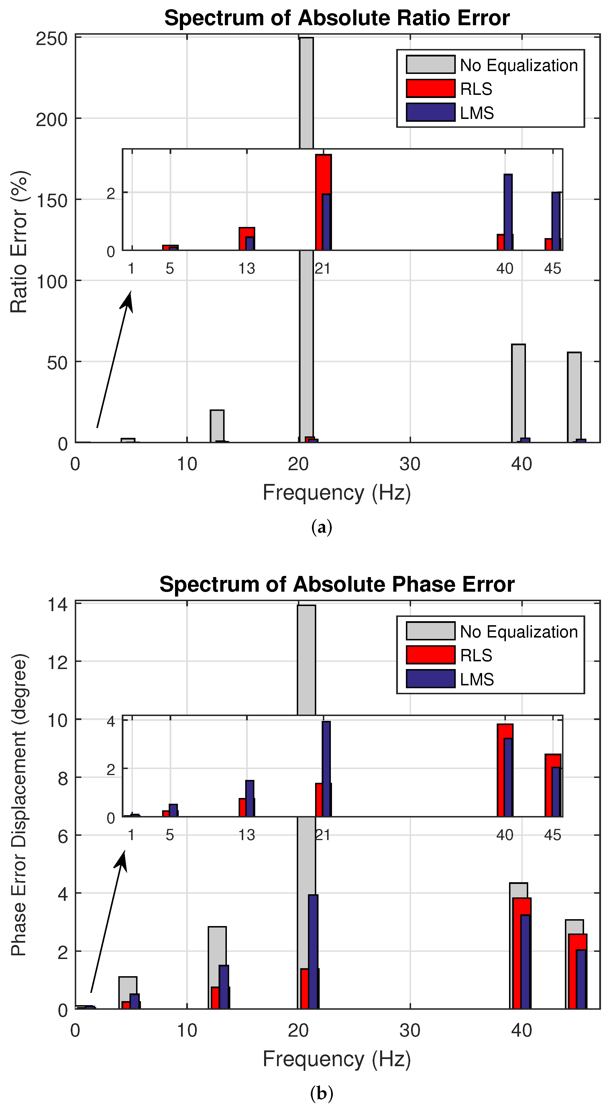
Blind Synthetic Experiments	Case 1	No Equalization	0.17	5.00	27.93	290.64	61.18	55.29
		RLS	0.00	0.03	0.24	2.15	0.12	0.14
		LMS	0.00	0.09	0.58	3.82	0.78	1.27
	Case 2	No Equalization	0.08	2.23	19.79	248.99	60.38	55.50
		RLS	0.00	0.01	0.07	1.46	0.55	0.44
		LMS	0.00	0.01	0.13	0.84	0.09	0.30
	Case 3	No Equalization	0.07	2.35	20.48	253.08	60.44	55.38
		RLS	0.00	0.03	0.26	2.25	0.05	0.21
		LMS	0.00	0.06	0.52	3.64	0.70	1.16
	Case 4	No Equalization	0.16	3.23	20.26	245.42	59.15	55.85
		RLS	0.00	0.40	1.53	4.87	2.87	1.30
		LMS	0.00	0.29	0.97	2.52	3.84	2.58
	Case 5	No Equalization	0.09	2.39	19.96	249.63	60.51	55.56
		RLS	0.00	0.16	0.78	3.29	0.54	0.39
		LMS	0.00	0.10	0.45	1.93	2.61	1.99
	Case 6	No Equalization	0.06	1.93	19.50	247.55	60.22	55.33
		RLS	0.00	0.04	0.43	2.13	1.55	0.78
		LMS	0.00	0.03	0.31	0.24	1.57	0.85
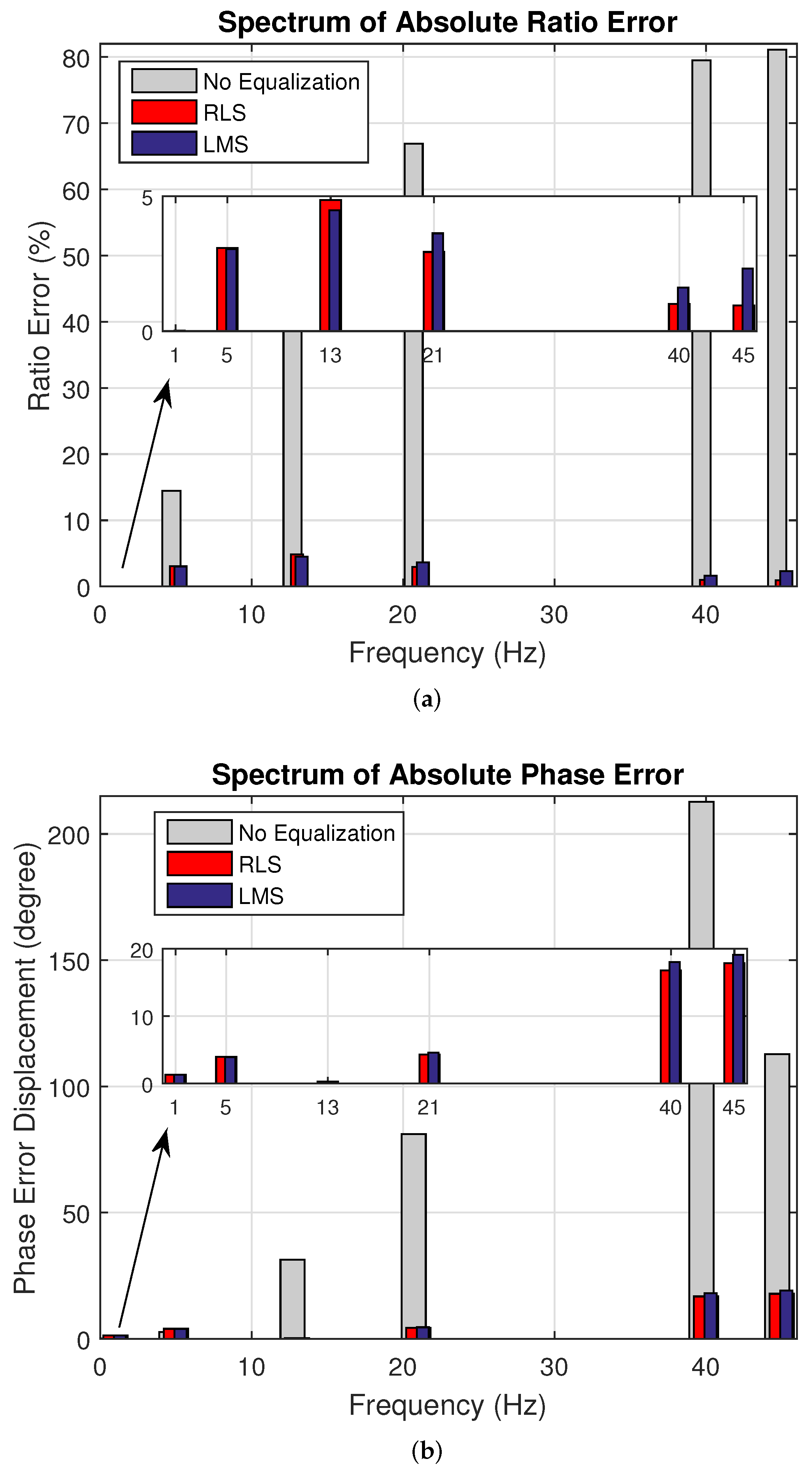
Blind Real Experiments	Case 7	No Equalization	0.04	14.43	50.00	66.46	79.27	80.79
		RLS	0.00	1.30	1.03	1.93	4.44	9.13
		LMS	0.04	0.39	2.04	4.52	4.24	9.52
	Case 8	No Equalization	0.01	14.44	49.72	66.88	79.50	81.10
		RLS	0.00	3.08	4.86	2.93	1.00	0.95
		LMS	0.01	3.04	4.48	3.62	1.61	2.32
	Case 9	No Equalization	0.05	14.38	49.46	66.97	79.70	80.98
		RLS	0.00	3.65	4.02	4.31	3.70	5.44
		LMS	0.05	4.55	3.67	0.52	3.62	8.77

and

Table 2. Results for Absolute Phase Error of the harmonic indices of the cases discussed.

Spectrum			Absolute Phase Error (Degree)
Harmonic Index			1	5	13	21	40	45
Blind Synthetic Experiments	Case 1	No Equalization	0.10	1.61	1.51	9.22	6.79	5.21
		RLS	0.02	0.17	0.51	0.24	2.34	1.52
		LMS	0.00	0.09	0.32	0.16	2.83	1.94
	Case 2	No Equalization	0.10	0.91	2.53	13.12	3.62	2.43
		RLS	0.04	0.23	0.70	0.61	2.06	1.28
		LMS	0.04	0.23	0.84	2.56	2.53	1.65
	Case 3	No Equalization	0.10	0.67	1.91	11.48	1.23	0.70
		RLS	0.02	0.15	0.47	0.07	2.15	1.38
		LMS	0.01	0.07	0.30	0.33	2.60	1.77
	Case 4	No Equalization	0.11	2.54	5.33	18.28	12.89	10.18
		RLS	0.03	0.35	0.90	0.38	4.05	2.69
		LMS	0.08	0.54	1.47	4.02	3.51	2.21
	Case 5	No Equalization	0.10	1.10	2.84	13.93	4.34	3.07
		RLS	0.03	0.24	0.74	1.37	3.82	2.57
		LMS	0.09	0.50	1.49	3.93	3.23	2.03
	Case 6	No Equalization	0.10	0.56	2.03	12.19	2.55	1.73
		RLS	0.10	0.51	1.63	3.14	4.71	3.01
		LMS	0.12	0.64	2.07	5.96	4.89	3.12
Blind Real Experiments	Case 7	No Equalization	0.15	2.61	31.90	278.51	147.56	112.69
		RLS	0.21	2.60	3.51	12.40	12.23	20.55
		LMS	0.24	1.14	1.82	4.97	11.98	20.72
	Case 8	No Equalization	0.18	2.64	31.33	81.07	212.77	112.80
		RLS	1.30	3.97	0.26	4.31	16.79	17.86
		LMS	1.30	3.93	0.24	4.58	18.02	19.09
	Case 9	No Equalization	0.15	2.30	31.57	80.73	212.16	112.77
		RLS	0.91	0.30	4.16	1.49	13.34	13.09
		LMS	1.29	1.01	3.72	2.06	14.28	11.82

. In this section, special emphasis is placed on Case 8, which is illustrated here for clarity.

Figure 12a,b depict the results of Case 8 in terms of absolute errors in ratio and phase. For this case, the ratio error values were below 5%, for both RLS and LMS. Without equalization, the ratio error values can reach up to 81.10% for higher-order harmonics. Regarding phase angles, the values for lower-order harmonics were below 5 degrees for both algorithms. However, for higher-order harmonics, the results improved compared to the case without equalization, with values close to 212 degrees, but they still did not reach the limit stipulated in the standard, remaining around 19 degrees.

Table 1 presents the values related to absolute ratio error, encompassing all cases analyzed. The absolute ratio error was computed by determining the difference between the ideal ratio and the equalized ratio for each harmonic of interest, as shown in Equation (2). Note that cases 1 through 6 (white part) represent the results for blind equalization of synthetic experiments. In cases 7 to 9 (grey part), blind equalization was applied to real experiments. Each case presents the results of the absolute ratio error, allowing for a comparison between the non-equalized scenario and the outcomes achieved with the RLS and LMS algorithms. In the simulated scenarios, covering Cases 1 to 6, the ratio results adhere to the parameters recommended by the IEC 61869-1 and IEC/TR 61869-103 standards. In contrast, in the context of the real experiment, it is noteworthy that in 91% of the cases, the ratio error remains below the established threshold of 5%, revealing significant compliance with the mentioned standard. This result is promising when compared to all cases without equalization, where the results meet the standard threshold in only 27% of the cases.

Table 2 presents the results related to the absolute phase error, encompassing all analyzed scenarios. The absolute phase error was calculated by comparing the ideal phase to the equalized phase for each harmonic of interest as shown in Equation (3). In each case, the absolute phase error results are presented, enabling a comparison between the non-equalized scenario and the results obtained with the RLS and LMS algorithms. In the simulated cases, the phase error remained equal to or below 5 degrees, in accordance with the requirements established by the standard. However, in the real cases, Cases 7, 8, and 9, the values obtained by the RLS and LMS algorithms recorded an error of less than 5 degrees in 64% of situations, in contrast to cases without equalization, where the standard threshold is met in only 33% of cases. It is worth noting that a degradation of results is observed at higher harmonic orders, adding complexity to the scenario.

It is worth emphasizing the results obtained through blind equalization, as this approach is able to achieve positive outcomes, even though it represents a methodologically challenging approach when compared to the other two alternatives. Blind equalization, despite its complexity, shows promise in addressing the equalization problem, particularly when combined with techniques like the Genetic Algorithm.

4.3. Online Equalization

To demonstrate the method’s adaptive capability under different temperature and burden conditions, a simple experiment was simulated. In Figure 13, the magnitude frequency response is presented for the transformer considered in Figure 5. Two distinct circuits with different resonances points are presented. These two resonances points were created by modifying the electrical characteristics of the circuit, but in practice, they could correspond to different temperatures and burden conditions. The input signal containing harmonics and additive Gaussian white noise was injected into the transducer, which now works as a linear time-varying system. Initially, during the equalization process, the transducer exhibits the frequency response characteristics in “Condition-A”, as shown in the Figure 13, and after some time, its frequency response changes to “Condition-B”. The equalization system operates continuously, generating the equalized curves referred to as RLS-A and RLS-B, respectivaly. Note that in this example, only the RLS method is shown, and only the magnitude response is presented. This example demonstrates that the method is capable of performing online and adaptive equalization.

5. Conclusions

In this paper, a contribution was made towards correcting the frequency response of instrument transformers used in harmonic measurement. The results underscore the remarkable capability of adaptive blind equalization using RLS or LMS algorithms, substantially enhancing the performance of the transducers in real-world scenarios.

Initially, the methodology was tested in a simulated environment, as evidenced by the results presented in Table 1 and Table 2. Subsequently, a laboratory setup was assembled to evaluate the methodology in real experiments. The obtained results were extremely promising. Notably, the results for the laboratory setup demonstrated a significant improvement in the transformers’ frequency response for 91% of the harmonics in the ratio error and 64% for phase displacement when compared to values obtained without equalization. In contrast, when the equalization is not applied, the frequency response met the acceptable criteria defined by the standard for 27% of the harmonics in the ratio error and 33% of the harmonics in the phase.

The results presented in Table 1 and Table 2 for the laboratory case may not have been as favorable as those of the simulated system due to several underlying assumptions. For instance, the noise used in the tests might have characteristics that deviate from ideal Gaussian white noise. Additionally, the impact of instrumentation noise represented in Figure 1, $\eta \left[n\right]$, was not considered and will be the object of future research.

It is worth highlighting that the features and construction of measuring transformers only influence the methodology in the following cases: (i) if the transducer is not minimum-phase; (ii) if the frequency response has more than one resonance frequency. For case (i), a possible solution is currently under investigation and includes the use of neural networks and nonlinear adaptive filters for equalization; as for case (ii), the current genetic algorithm is configured to search for the first resonance frequency only and, therefore, should be adapted for more critical cases that encompass multiple resonance frequencies.

The utilization of adaptive filtering for blind equalization of transducers emerges as a highly promising research area. For example, the extensive number of instrumentation transformers designed for measuring the fundamental component with excellent accuracy, installed worldwide, can be utilized for harmonic phasor measurement after equalization. The methodology, for instance, can be integrated into future versions of the MU (Merging Unit) that may enable the installed transformers to self-equalize autonomously.

References

- Castello, P.; Laurano, C.; Muscas, C.; Pegoraro, P.A.; Toscani, S.; Zanoni, M. Harmonic Synchrophasors Measurement Algorithms with Embedded Compensation of Voltage Transformer Frequency Response. IEEE Trans. Instrum. Meas. 2021, 70, 9001310. [Google Scholar] [CrossRef]
- Verhelst, B.; Rens, S.; Rens, J.; Knockaert, J.; Desmet, J. On the Remote Calibration of Instrumentation Transformers: Influence of Temperature. Energies 2023, 16, 4744. [Google Scholar] [CrossRef]
- Artale, G.; Caravello, G.; Cataliotti, A.; Cosentino, V.; Cara, D.D.; Guaiana, S.; Panzavecchia, N.; Tine, G. Measurement of Simplified Single- And Three-Phase Parameters for Harmonic Emission Assessment Based on IEEE 1459–2010. IEEE Trans. Instrum. Meas. 2021, 70, 9000910. [Google Scholar] [CrossRef]
- D’Avanzo, G.; Faifer, M.; Landi, C.; Laurano, C.; Letizia, P.S.; Luiso, M.; Ottoboni, R.; Toscani, S. Improving Harmonic Measurements with Instrument Transformers: A Comparison among Two Techniques. In Proceedings of the Conference Record—IEEE Instrumentation and Measurement Technology Conference, Glasgow, UK, 17–20 May 2021; pp. 1–6. [Google Scholar] [CrossRef]
- Faifer, M.; Laurano, C.; Ottoboni, R.; Toscani, S. Adaptive Polynomial Harmonic Distortion Compensation in Current and Voltage Transformers Through Iteratively Updated QR Factorization. IEEE Trans. Instrum. Meas. 2023, 72, 9001810. [Google Scholar] [CrossRef]
- Faifer, M.; Ferrero, A.; Laurano, C.; Ottoboni, R.; Toscani, S.; Zanoni, M. An Innovative Approach to Express Uncertainty Introduced by Voltage Transformers. IEEE Trans. Instrum. Meas. 2020, 69, 6696–6703. [Google Scholar] [CrossRef]
- Crotti, G.; D’Avanzo, G.; Landi, C.; Letizia, P.S.; Luiso, M. Evaluation of Voltage Transformers’ Accuracy in Harmonic and Interharmonic Measurement. IEEE Open J. Instrum. Meas. 2022, 1, 9000310. [Google Scholar] [CrossRef]
- Stiegler, R.; Freiburg, M.; von Zyl, J.; Meyer, J.; Feustel, F.; German, C. Methods for on-site qualification and calibration of inductive instrument voltage transformers for harmonic measurements. In Proceedings of the CIRED 2021—The 26th International Conference and Exhibition on Electricity Distribution. Institution of Engineering and Technology, Online Conference, 20–23 September 2021; pp. 752–756. [Google Scholar] [CrossRef]
- Beug, M.F.; Kolling, A.; Moser, H. A New Calibration Transformer and Measurement Setup for Bridge Standard Calibrations Up To 5 kHz. IEEE Trans. Instrum. Meas. 2017, 66, 1531–1538. [Google Scholar] [CrossRef]
- Jaschke, C.; Schegner, P. A measuring system to identify the frequency response of high current instrument transformers. In Proceedings of the 2015 Modern Electric Power Systems (MEPS), Wroclaw, Poland, 6–9 July 2015; pp. 1–6. [Google Scholar] [CrossRef]
- Hu, H.; Xu, Y.; Wu, X.; Lin, F.; Xiao, X.; Lei, M. Passive-compensation clamp-on two-stage current transformer for online calibration. IET Sci. Meas. Technol. 2021, 15, 730–737. [Google Scholar] [CrossRef]
- Letizia, P.S.; Crotti, G.; Mingotti, A.; Tinarelli, R.; Chen, Y.; Mohns, E.; Agazar, M.; Istrate, D.; Ayhan, B.; Çayci, H.; et al. Characterization of Instrument Transformers under Realistic Conditions: Impact of Single and Combined Influence Quantities on Their Wideband Behavior. Sensors 2023, 23, 7833. [Google Scholar] [CrossRef] [PubMed]
- Agazar, M.; Istrate, D.; Pradayrol, P. Evaluation of the Accuracy and Frequency Response of Medium-Voltage Instrument Transformers under the Combined Influence Factors of Temperature and Vibration. Energies 2023, 16, 5012. [Google Scholar] [CrossRef]
- Stiegler, R.; Meyer, J. Impact of external influences on the frequency dependent transfer ratio of resin cast MV voltage instrument transformers. In Proceedings of the International Conference on Harmonics and Quality of Power, ICHQP, Naples, Italy, 29 May–1 June 2022; pp. 1–6. [Google Scholar] [CrossRef]
- Mingotti, A.; Costa, F.; Peretto, L.; Tinarelli, R. Effects on the Accuracy Performance of Rogowski Coils Due to Temperature and Humidity. In Proceedings of the Conference Record—IEEE Instrumentation and Measurement Technology Conference, Ottawa, ON, Canada, 16–19 May 2022; pp. 1–6. [Google Scholar] [CrossRef]
- Cesky, L.; Janicek, F.; Kubica, J.; Skudrik, F. Overheating of primary and secondary coils of voltage instrument transformers. In Proceedings of the 2017 18th International Scientific Conference on Electric Power Engineering, EPE 2017, Kouty nad Desnou, Czech Republic, 17–19 May 2017; pp. 1–6. [Google Scholar] [CrossRef]
- Gopp, D.; Sperling, E.; Bischof, T.; Krüger, M. Temperature dependency of the frequency response characteristic of high voltage inductive instrument transformers and RC dividers. In Proceedings of the 22nd International Symposium on High Voltage Engineering (ISH 2021), Institution of Engineering and Technology, Xi’an, China, 21–26 November 2021; pp. 1664–1669. [Google Scholar] [CrossRef]
- Dadić, M.; Župan, T.; Kolar, G. FIR modeling of voltage instrument transformers from frequency response data. In Proceedings of the 2018 1st International Colloquium on Smart Grid Metrology, SmaGriMet 2018, Split, Croatia, 24–27 April 2018; Number 3; pp. 1–6. [Google Scholar] [CrossRef]
- Zhao, B.; Liu, H.; Zhang, P.; Bi, T.; Qian, C. Instrument Transformer Calibration Method Based on Synchrophasor Measurement. In Proceedings of the I and CPS Asia 2022—2022 IEEE IAS Industrial and Commercial Power System Asia, Shanghai, China, 8–11 July 2022; pp. 179–184. [Google Scholar] [CrossRef]
- Vaytelenok, L. Operation of relay protection digital elements at saturation of current transformers: Modeling and analysis. In Proceedings of the 2019 International Conference on Industrial Engineering, Applications and Manufacturing, ICIEAM 2019, Sochi, Russia, 25–29 March 2019; pp. 1–6. [Google Scholar] [CrossRef]
- Cui, B.; Srivastava, A.K.; Banerjee, P. Synchrophasor-Based Condition Monitoring of Instrument Transformers Using Clustering Approach. IEEE Trans. Smart Grid 2020, 11, 2688–2698. [Google Scholar] [CrossRef]
- Sidorova, A.; Litvinov, I.; Kornilovich, D.; Fedorova, V.; Tanfilev, O.; Titov, V. Development and Verification of an Advanced Method for Diagnosing Measuring Transformers. In Proceedings of the 2021 Ural-Siberian Smart Energy Conference, USSEC 2021, Novosibirsk, Russia, 13–15 November 2021; pp. 57–61. [Google Scholar] [CrossRef]
- Kaczmarek, M.; Stano, E. Challenges of Accurate Measurement of Distorted Current and Voltage in the Power Grid by Conventional Instrument Transformers. Energies 2023, 16, 2648. [Google Scholar] [CrossRef]
- Toscani, S.; Faifer, M.; Ferrero, A.; Laurano, C.; Ottoboni, R.; Zanoni, M. Compensating Nonlinearities in Voltage Transformers for Enhanced Harmonic Measurements: The Simplified Volterra Approach. IEEE Trans. Power Deliv. 2021, 36, 362–370. [Google Scholar] [CrossRef]
- Collin, A.J.; Femine, A.D.; Gallo, D.; Langella, R.; Luiso, M. Compensation of Current Transformers’ Nonlinearities by Tensor Linearization. IEEE Trans. Instrum. Meas. 2019, 68, 3841–3849. [Google Scholar] [CrossRef]
- D’Avanzo, G.; Faifer, M.; Landi, C.; Laurano, C.; Letizia, P.S.; Luiso, M.; Ottoboni, R.; Toscani, S. Theory and Experimental Validation of Two Techniques for Compensating VT Nonlinearities. IEEE Trans. Instrum. Meas. 2022, 71, 9001312. [Google Scholar] [CrossRef]
- Faifer, M.; Laurano, C.; Ottoboni, R.; Toscani, S.; Zanoni, M. Harmonic Distortion Compensation in Voltage Transformers for Improved Power Quality Measurements. IEEE Trans. Instrum. Meas. 2019, 68, 3823–3830. [Google Scholar] [CrossRef]
- Cataliotti, A.; Cosentino, V.; Crotti, G.; Femine, A.D.; Di Cara, D.; Gallo, D.; Giordano, D.; Landi, C.; Luiso, M.; Modarres, M.; et al. Compensation of Nonlinearity of Voltage and Current Instrument Transformers. IEEE Trans. Instrum. Meas. 2019, 68, 1322–1332. [Google Scholar] [CrossRef]
- Resende, D.F.; Duque, C.A.; Nepomuceno, E.G.; Lima, M.A.A.; Silva, L.R.M. Adaptive Channel Equalization for Frequency Response Correction of Instrument Transformers. In Proceedings of the 20th International Conference on Harmonics and Quality of Power—ICHQP, Naples, Italy, 29 May–1 June 2022; pp. 1–6. [Google Scholar] [CrossRef]
- Chi, C.Y.; Feng, C.C.; Chen, C.H.; Chen, C.Y. Blind Equalization and System Identification: Batch Processing Algorithms, Performance and Applications; Springer Science & Business Media: London, UK, 2006; p. 478. [Google Scholar] [CrossRef]
- Zhan, Z.H.; Shi, L.; Tan, K.C.; Zhang, J. A survey on evolutionary computation for complex continuous optimization. Artif. Intell. Rev. 2022, 55, 59–110. [Google Scholar] [CrossRef]
- Holland, J.H. Adaptation in Natural and Artificial Systems; University of Michigan Press: Ann Arbor, MI, USA, 1976; p. 529. [Google Scholar]
- Goldberg, D.E. Genetic Algorithms in Search, Optimization, and Machine Learning; Addison-Wesley: Reading, MA, USA, 1989; p. 412. [Google Scholar]
- Raj, A.; Kumar, A.; Sharma, V.; Rani, S.; Shanu, A.K.; Singh, T. Applications of Genetic Algorithm with Integrated Machine Learning. In Proceedings of the 2023 3rd International Conference on Innovative Practices in Technology and Management, ICIPTM 2023, Uttar Pradesh, India, 22–24 February 2023; pp. 1–6. [Google Scholar] [CrossRef]
- IEC 61869-1; Instrument Transformers—Part 1: General Requirements. Technical report; IEC—International Electrotechnical Commission: Geneva, Switzerland, 2007.
- TR 61869-103; Instrument Transformers—The Use of Instrument Transformers for Power Quality Measurement. Technical report; IEC—International Eectrotechnical Commission: Geneva, Switzerland, 2012.