Validation Aspects for Grid-Forming Converters Based on System Characteristics and Inertia Impact

Abstract

Grid-forming converters are considered a key technology for electrical grids with a high share of renewable energy. However, there is a lack of a general, robust and verifiable definition of what constitutes this behaviour. Therefore, this paper presents three simple scenarios that enable such a definition. They are based on simple black-box simulations that allow manufacturers to protect their development work. It can be shown that grid forming can be clearly distinguished from grid-following controls by their grid behaviour in the proposed scenarios. Extensive results illustrate this and also provide suggestions to deepen the understanding of grid-forming grid behaviour and its impact on system inertia. These findings should inspire the development of a clear definition and ultimately new requirements for converter systems.

1. Introduction

The goal of achieving a climate-neutral energy sector in the future leads to a transformation of energy generation. This results in the challenge of compensating not only for the loss of generation power, but also for the decrease in system services provided by conventional power plants. In particular, the decrease in inertia in the grid is considered to be one of the biggest risks by transmission system operators (TSOs) [1].

The reason for this is that reduced inertia in the power system results in a weak grid frequency and thus can cause larger and faster frequency deviations and increase the number of critical events in the grid; in the worst case, the system splits [2].

Therefore, it can be assumed that in the future, system inertia will not only be provided conventionally by synchronous generators, but also by inverter-based resources (IBRs) [3]. Grid-forming (GFM) converters have shown that they are able to provide (virtual) inertia when equipped with sufficient and dynamic energy storage, unlike existing grid-following (GFL) converters [4]. Thus, it is essential for grids with a high share of IBRs to use GFM converters [5].

However, there is still no consensus in the scientific community as to what exactly constitutes a GFM converter [6]. In addition to the lack of verification procedures, which will be discussed later, different terminologies are used. Besides the common terms GFM and GFL, “grid-leading” is used in [7] for island grids, “grid-feeding” is used in [8] for GFL, and “grid-supporting” (GSP) is used for different variations in GFM and grid feeding of the respective GFL.

A suggestion was made in [9] that the terminology should take into account not only virtual inertia provided by the control principle, but also additional functionalities such as the possibility to provide primary control power. Therefore, in addition to GFM and GFL, the terms GSP and grid stabilising (GSB) were chosen to describe the converter behaviour. The control principle receives a separate description, which is now divided into grid-voltage-following (GVFL) and grid-voltage-forming (GVFM). The description of the terminology is shown in

Table 1. Converter terminology that is used in this work [9].

Converter Behaviour	Grid-Following	Grid-Supporting	Grid-Stabilising	Grid-Forming
	(GFL)	(GSP)	(GSB)	(GFM)
Additional	None	$P\left(f\right)$ + Energy	$Q\left(V\right)$	$P\left(f\right)$ + Energy 2
Functionalities		$Q\left(V\right)$	(Limited Inertia) 1	$Q\left(V\right)$
Control Principle	Grid-Voltage-Following (GVFL)		Grid-Voltage-Forming (GVFM)
	(No Inertia)		(Inertia $f\left(P\right)$)
Control Method	Current Control,		VSM, Droop-Control,
	Hysteresis Control…		Direct Voltage Control…

¹ Inherent active power provision is limited due to energy storage capability; inherent reactive power provision is possible. ² Energy must be available instantaneously.

.

The advantage of this terminology is that the intended use of the converter system is taken into account, and thus, inaccuracies in the description are also eliminated. When talking about a GFM STATCOM, for example, this is actually not an adequate description, as a STATCOM does not have any significant energy that would let it form a grid. In contrast, using the proposed terminology, it can be said that it is operated with a GVFM control principle, which makes the system GSB.

In addition, the conventional GFL behaviour can be described separately from the use of a GVFL control with primary control and energy reserves. This offers advantages for the grid, which are additionally rewarded by the terminology. At the same time, however, a clear separation between native inertia and controllable (fast) primary control is evident.

The differences between the various converter behaviours are contrasted and analysed in this paper. The aim of this is to deepen the understanding of converter behaviour and to work towards a clear definition that distinguishes undoubtedly between GVFM and GVFL.

What is generally understood is that GVFL converter controls inherently behave like a controlled current source, while GVFM controls inherently have the same behaviour as a controlled voltage source [10]. In addition to this simple but very general definition, [11] compares further requirements that are placed on GVFM controls in various pieces of the literature. The different requirements identified as most frequently requested are as follows:

• Fault-ride-through (FRT) capability.
• Positive effect on system effective inertia and frequency response.
• Voltage stabilisation and reactive power support.
• Black-start capability.

Although these are all desirable aspects, only the second point serves to characterise GVFM control principles. While the first and third points could also be fulfilled by GVFL control methods, the fourth point requires an external energy supply in addition to GVFM control.

In [5], four types are presented that could define GVFM behaviour. These are as follows:

• Specification of an exact control procedure.
• Reference curves (e.g., active and reactive power) that must be met precisely.
• Frequency domain impedance measurements.
• Reference scenarios in which only GFM converters can remain stable.

While the first two options are rightly not recommended because they either interfere too much with manufacturers’ development or depend too much on control parameters, the last two points are conceivable. However, reference scenarios are given for the last proposal, e.g., island grids, which again could only be operated with sufficient energy. Scenarios in weak networks are also avoided in this paper because the very term “weak network” is a subject of debate. Instead, the focus is on how the voltage and current source behaviour of the inverters can be visualised and verified.

This work contributes to achieving this. For this purpose, two reference scenarios are proposed that have different complexity and can demonstrate different effects. Still, both are able to make a clear distinction between GVFM and GVFL when the implementation of the scheme in a test model is unknown. Based on this, the reference scenarios are evaluated, which are intended to enable verification methods for GVFM converter controls in test environments. Therefore, the visualisations in this paper are for demonstration purposes first. Ultimately, however, the methodology is intended to be used in validations of manufacturer models.

In addition, we will analyse how the traditional measure of inertia can be measured and understood in converter networks and what it can express and what it can not.

The work is structured as follows: Section 2 illustrates which grid models are used, what control methods are simulated exemplarily and how the measurements are realised. Subsequently, extensive results of these measurements are shown and explained in Section 3. Section 4 discusses which findings can be drawn from which measurements. Finally, the work is concluded in Section 5 and it is described what this work means for future research.

2. Modelling and Measurement Techniques

This section explains how to run the simulations and take the measurements. The aim is to keep the simulation effort and the complexity of the models as low as possible. Two grid equivalents and a total of three different control methods are used. Since the models are treated like black box models that do not allow insight, measured variables on the converter are calculated and not measured. A rotating coordinate system is used for the results, which simplifies visualisation. Finally, it is explained how the inertia H is measured.

2.1. Grid Model

As an example, in this study, a survey is made of a converter that could be used in a wind turbine. In the following, the topology and the two grid equivalents are explained.

2.1.1. Topology

The topology used is shown in Figure 1. The converter is connected to the grid via an LC filter and a transformer. It is assumed that the filter parameters are known, but only measurements at the point-of-common-coupling (PCC) are possible.

The converter has a rated power and rated voltage of $4.25$ MVA and 660 V, respectively. This topology serves only as one possible use case but is orientated towards a real certification process. Other applications and filters are equally conceivable and the analyses presented are also applicable. The most relevant parameters of the test system are given in

Table A1. Relevant parameters of the used grid and converter model.

Grid Parameters
Description	Value	Unit
Nominal grid power	$S_{\mathrm{nG}}=40$	MVA
Nominal grid frequency	$f_{\mathrm{n}}=50$	Hz
Nominal grid voltage	$v_{\mathrm{nG}}=33$	kV
Inertia constant	$H_{\mathrm{G}}=4.5$	s
Active power reference	$p_{\mathrm{G}}^{★}=0$	pu
Active power droop	$D_{f{p}_{\mathrm{G}}}=0.03$	pu
Active power droop	$D_{\widehat{v}{q}_{\mathrm{G}}}=0.03$	pu
Short-Circuit-Ratio	$\mathrm{SCR}=10$
Impedance Ratio	$R_{\mathrm{G}}/X_{\mathrm{G}}\approx 0.1$
Converter  Parameters
Description	Value	Unit
Nominal converter power	$S_{\mathrm{nC}}=4.25$	MVA
Nominal converter voltage	$v_{\mathrm{nC}}=660$	V
Active power reference	$p_{\mathrm{C}}^{★}=0$	pu
Reactive power reference	$q_{\mathrm{C}}^{★}=0$	pu

in the Appendix A.

2.1.2. Converter Voltage and Current Calculation

In order to obtain the measured variables at the converter, back calculations must be performed with knowledge of the filter variables. In principle, it would be possible to carry out these calculations with complex numbers. In this case, this is not possible because a dynamic and exact measurement of the grid frequency ${\omega }_{\mathrm{G}}$ is required. In order to be able to represent the transient processes exactly, a rough estimate of the frequency is not sufficient. The challenges of such a frequency measurement are described in Section 2.4. In summary, the complex calculation is not recommended here and the differential equations must be set up. The voltages in Figure 1 can be expressed as:

$$v_{\mathrm{PCC}}=v_{R_{\mathrm{pF}}}+v_{C_{\mathrm{pF}}}=R_{\mathrm{pF}}{i}_{\mathrm{pF}}+v_{C_{\mathrm{pF}}}$$

(1)

where $i_{\mathrm{pF}}=C_{\mathrm{pF}}{\displaystyle \frac{d{v}_{C_{\mathrm{pF}}}}{dt}}$. Equation (1) can then also be written as:

$${\displaystyle \frac{d{v}_{C_{\mathrm{pF}}}}{dt}}={\displaystyle \frac{1}{R_{\mathrm{pF}}{C}_{\mathrm{pF}}}}(v_{\mathrm{PCC}}-v_{C_{\mathrm{pF}}})$$

(2)

On the other hand, the currents in Figure 1 add up to:

$$i_{\mathrm{C}}=i_{\mathrm{PCC}}+i_{\mathrm{pF}}=i_{\mathrm{PCC}}+C_{\mathrm{pF}}{\displaystyle \frac{d{v}_{C_{\mathrm{pF}}}}{dt}}$$

(3)

This equation can be solved because $i_{\mathrm{PCC}}$ is measured and ${\displaystyle \frac{d{v}_{C_{\mathrm{pF}}}}{dt}}$ can be calculated via Equation (2) where all variables are known. This also allows the converter voltage to be calculated via the series branch:

$$v_{\mathrm{C}}=R_{\mathrm{sF}}{i}_{\mathrm{C}}+L_{\mathrm{sF}}{\displaystyle \frac{d{i}_{\mathrm{C}}}{dt}}+v_{\mathrm{PCC}}$$

(4)

The calculation of the converter values is shown in the signal flow diagram in Figure 2.

This method is validated in Section 3.1.

2.1.3. Grid Equivalent

In this study, the grid equivalent is used to create reference scenarios that the converter system runs through. The cases most frequently used for this purpose include phase and amplitude jumps of the grid voltage. A controlled voltage source behind a grid impedance is sufficient for this. However, these scenarios are not realistic, as they only represent selected processes and not the entire system.

A more realistic approach is to simplify the behaviour of the electrical power grid and also bring it into the test environment via a controlled voltage source, as was carried out in [12]. Here, the previous behaviour of the grid is represented, which is significantly influenced by the synchronous machine. In modern, converter-dominated grids, this assumption is less accurate. However, it allows for frequency deviations in studies such as this one and makes the impact of the inverter on the frequency visible.

The replica of the electrical power grid is shown in Figure 3.

As can be seen, the inertia H can be adjusted in the swing equation. Additionally, the grid also provides primary control in the form of a $P\left(f\right)$ droop that can be tuned with the parameter $D_{f{P}_{\mathrm{G}}}$. Both the $P\left(f\right)$ droop and the measurement of the voltage amplitude are filtered by a first-order delay. In addition to this, there is another filter in the voltage control that represents the excitation time constant ${\tau }_{{\mathrm{E}}_{\mathrm{G}}}$.

The scenario here consists of a load ${\underline{Z}}_{\mathrm{Load}}$ that is connected in parallel to the grid and the converter. This creates a realistic frequency drop that both the grid and the inverter can contribute to stabilising.

In contrast, the second grid equivalent consists of a simple controlled voltage source without a closed control loop, as Figure 4 illustrates.

Here, the grid frequency, amplitude and phase of the voltage can be changed by given values. In this study, this is carried out with alterations of ${\widehat{v}}_{\mathrm{G}}^{*}$ and ${\phi }_0$.

2.2. Control Methods

Today, there is a wide variety of converter controls [13,14]. The most common GVFL control is the current control in the synchronous reference frame (SFR) as presented in [15,16]. It is used as the GVFL control in this work and is shown in Section 2.2.1. The most popular GVFM controls, on the other hand, are the droop control and the virtual synchronous machine (VSM) [17,18,19,20], which have the same inner control structure and whose synchronisation unit can also be identical in certain versions [21].

A different GVFM control is presented in [12,22]. It is explained in Section 2.2.2. Thereafter, the VSM, which serves the purpose of comparing different GVFM controls in this work, is illustrated in Section 2.2.3.

2.2.1. Current Control

The main task of the current control is to realise the higher-level power specifications as dynamically as possible. For this purpose, the control runs in a rotating coordinate system that rotates with the identified phase angle ${\theta }_{\mathrm{PLL}}$. This makes it easy to compare the reference current $i_{\mathrm{C},\mathrm{dq}}^{★}$ with the measured current $i_{\mathrm{C},\mathrm{dq}}$ and control it with a PI controller. The voltage difference calculated by the PI controller $\Delta v_{\mathrm{PI},\mathrm{dq}}$ is added to the grid voltage $v_{\mathrm{PCC},\mathrm{dq}}$ and the filter voltages in the feedforward (FF) control as Equation (5) shows.

$$v_{\mathrm{m},\mathrm{d}}=\Delta v_{\mathrm{PI},\mathrm{d}}+v_{\mathrm{PCC},\mathrm{d}}+r_{\mathrm{sF}}{i}_{\mathrm{C},\mathrm{d}}-l_{\mathrm{sF}}{i}_{\mathrm{C},\mathrm{q}}$$

(5a)

$$v_{\mathrm{m},\mathrm{q}}=\Delta v_{\mathrm{PI},\mathrm{q}}+v_{\mathrm{PCC},\mathrm{q}}+r_{\mathrm{sF}}{i}_{\mathrm{C},\mathrm{q}}+l_{\mathrm{sF}}{i}_{\mathrm{C},\mathrm{d}}$$

(5b)

Here, the filter resistance and the filter inductance are written in lower case because they are in the per-unit system.

The reference voltage $v_{\mathrm{m},\mathrm{dq}}$ is transformed back into the stationary coordinate system and passed on to the modulation of the converter. The control scheme of the current control is given in Figure 5.

As can be observed, the control is heavily dependent on the measured grid voltage and its phase angle identification by the phase-locked loop (PLL). With this design it cannot run in stand-alone operation.

2.2.2. Grid-Voltage-Forming Control (HSD-Control)

The idea behind this GVFM control is to predefine a reference voltage $v_{\mathrm{PCC}}^{★}$ and synchronise it slowly with the measured voltage. This has the advantage that it is not necessarily dependent on the measured voltage. Should the converter fall into an island, it would still be able to provide a voltage due to the internal voltage. The same applies to scenarios where the grid voltage is very weak.

Although identification of the phase angle and amplitude of the grid voltage is also necessary for this synchronisation, this is not problematic because a sliding discrete Fourier transform (sDFT) is used instead of the conventional SRF-PLL. This sDFT also has an identification that is inert and robust, especially in the presence of harmonic distortion, and therefore does not have the problems of the SRF-PLL. A detailed explanation of the sDFT is given in [23].

Another difference is that the control is not operated in the dq coordinate system, but with complex variables that are identified via the symmetrical components (SC). In addition to identifying the harmonics, this enables explicit control of the zero and negative sequence components.

Furthermore, no current controllers are implemented. The synchronisation voltage is only passed through a complex feedforward before the inverse SC and the inverse DFT. The control scheme is shown in Figure 6.

The core of the control is the synchronisation unit, whose function has already been described above. The calculation of $v_{\mathrm{sync}}={\widehat{v}}_{\mathrm{sync}}·{\mathrm{e}}^{\mathrm{j}{\phi }_{\mathrm{sync}}}$ can be seen in Figure 7.

This illustrates that the control target is not to synchronise the measured voltage with the reference voltage. It is to synchronise the synchronisation voltage, which is lagged via a delay (${\mathrm{z}}^{-1}$), with the measured voltage. In grid-connected operation, the reference voltage only serves as feedforward control, but would ensure the conservation of the synchronisation voltage in the case of islanding. The PI controllers have a P component $\approx 0$, while the inertia of the converter can be set via the I component.

In addition, the power can also be controlled here. Since the power controllers are not part of the synchronisation as in the VSM, their dynamics can be adjusted independently of the inertia of the control. This means that the dynamics in response to external changes are different here than with internal changes.

The implementation of the frequency synchronisation is analogous and can be seen in Figure 8.

The result is that the internal variables $v_{\mathrm{sync}}$ and ${\omega }_{\mathrm{sync}}$ are decoupled from the external influences. This yields the inertia of the voltage vector and the synchronisation frequency, which is desired in GVFM controls.

2.2.3. Virtual Synchronous Machine

This effect is achieved in the VSM through a different approach. Here, the synchronisation is implemented via the swing equation of the synchronous machine. The calculated synchronisation angle ${\theta }_{\mathrm{apc}}$ is used to transform the input variables into the rotating dq coordinate system and to transform the calculated reference voltage back into the stationary coordinate system. In between, there are subordinate voltage and current controls that dynamise the inertia properties of the synchronous machine and make it suitable for a converter. The design used in this work is taken from [20] and is shown in Figure 9.

Here, it can be seen that no PLL is necessary for the control. It can be used additionally to deliver grid control power in the form of $P\left(f_{\mathrm{PLL}}\right)$, but this is also possible with the internal frequency $f_{\mathrm{apc}}$. It is therefore only necessary to connect the converter to the grid initially, and no longer during grid operation.

The active power control (APC) that calculates the synchronisation angle ${\theta }_{\mathrm{apc}}$ and the frequency ${\omega }_{\mathrm{apc}}$ is shown in Figure 10.

Due to the similar approach, the similarity with the grid model used in Figure 3 can be seen. In this implementation, an additional primary control was deliberately avoided to make it more comparable. The inertia can be adjusted via H. This inertia affects both changes in the grid measured by p as well as changes in the reference power $p^{★}$. While the former is desirable, the latter is not necessarily wanted.

The implementation of the reactive power control is presented in Figure 11.

In this design, a $v\left(q\right)$ droop is implemented to stabilise the amplitude of the grid voltage. However, there is no inertia here to keep the voltage vector constant during transient changes. The resulting voltage vector of the converter voltage is mainly determined by the subordinate control. While there are other implementations, this is one of the most popular. The effect of the lack of inertia with respect to the voltage amplitude is shown in Section 3.6.

2.3. Rotating Reference Frame

When talking about the voltage phase angle, the angle of the complex voltage vector is usually meant. It must first be understood how the complex voltage vector is composed. The Clark transformation transforms a symmetrical, three-phase voltage into the two components $\alpha$ and $\beta$:

$$\left(\begin{array}{c}{v}_{\alpha }\\ v_{\beta }\end{array}\right)={\displaystyle \frac{2}{3}}\left(\begin{array}{ccc}1& -\frac{1}{2}& -\frac{1}{2}\\ 0& \frac{\sqrt{3}}{2}& -\frac{\sqrt{3}}{2}\end{array}\right)\left(\begin{array}{c}{v}_{\mathrm{a}}\\ v_{\mathrm{b}}\\ v_{\mathrm{c}}\end{array}\right)$$

(6)

Based on this, the complex voltage vector

$$\underline{v}=v_{\alpha }+\mathrm{j}{v}_{\beta }=\widehat{v}·{\mathrm{e}}^{\mathrm{j}\theta }$$

(7)

can be formed. With a symmetrical, undistorted voltage, $v_{\alpha }$ and $v_{\beta }$ are sinusoidal and the voltage vector rotates with the angular grid frequency. This makes it difficult to observe the phase angle $\theta$, as it changes with a constant gradient. Therefore, in this paper, $\theta$ is separated into its two components:

$$\theta =\omega t+\phi$$

(8)

Since the stationary phase angle $\phi$ is of interest, a coordinate system is chosen that rotates with the angular frequency $\omega$. In this coordinate system the phase angle is stationary constant and only changes in angle beyond the constant frequency result in a change.

Figure 12 illustrates this method.

Observe how the xy reference frame continues to rotate at constant angular frequency after a provoked change. This means that the angular frequency is the last measured frequency before the events that are simulated in the reference scenarios like load change and phase jump. This rotating reference frame is chosen for all results concerning the phase angle. This is indicated by the use of $\phi$ instead of $\theta$ and $v_{\mathrm{x}}$ and $v_{\mathrm{y}}$ instead of $v_{\alpha }$ and $v_{\beta }$.

2.4. Inertia Measurement

The inherent effect of a load change in the grid on the grid frequency is determined by the accumulated inertia of the grid. Thus, inertia can be measured as an instantaneous response proportional to the rate-of-change-of-frequency (RoCoF) [24]. Synthetic inertia, on the other hand, can also be measured after more than one grid period [25]. Here, however, it will first be derived and explained how inertia H can classically be measured in the grid.

The inertia H is defined as the ratio between stored energy $E_{\mathrm{kin}}=\frac{1}{2}J{\omega }_{\mathrm{r}0}^2$ at synchronous frequency ${\omega }_{\mathrm{r}0}$ and nominal power $S_{\mathrm{b}}$:

$$H=\frac{1}{2}{\displaystyle \frac{J{\omega }_{\mathrm{r}0}^2}{S_{\mathrm{b}}}}$$

(9)

Following a change in torque T of the machine, the deviation can be calculated by

$$\Delta T=J\frac{d{\omega }_{\mathrm{r}}}{dt}$$

(10)

while the relation between torque and power P in this case is

$$\Delta P={\omega }_{\mathrm{r}}\Delta T$$

(11)

with ${\omega }_{\mathrm{r}}=2\pi f_{\mathrm{r}}$ and

$$f=\frac{p_f}{2}{f}_{\mathrm{r}}$$

(12)

with f being the electric frequency [24].

Incorporating (10) and (11) in (9) leads to

$$2H{\displaystyle \frac{S_{\mathrm{b}}}{{\omega }_{\mathrm{r}0}}}\frac{d{\omega }_{\mathrm{r}}}{dt}=\Delta P$$

(13)

which can be written as:

$$H={\displaystyle \frac{\frac{\Delta P}{S_{\mathrm{b}}}}{2\frac{df}{dt}\frac{1}{f_0}}}$$

(14)

with $f_0$ being the nominal grid frequency $f_0=f_{\mathrm{n}}$.

If there is knowledge of how large the load change $\Delta P$ is, the measured RoCoF can be used to calculate the inertia of the grid. In simulations, this can be carried out rather easily, while inertia measurements in the real grid are more complicated and less precise. One of the first investigations in which this was carried out is [26]. More recently, a measurement was carried out on the British grid [27]. Overviews of inertia measurement techniques and challenges are given in [28,29,30]. Some of the issues are [27]:

• Measurement of load change.
• Identification of the event.
• Frequency and RoCoF measurement.

While the first two aspects are not as difficult in simulations, the frequency measurement is also not trivial. Possible frequency measurements are deriving the phase angle of the voltage space vector [27] or measuring the rotational speed of a nearby synchronous generator [31,32]. Since the former can be distorted even in simulation and filters could falsify the RoCoF, the latter is used.

Therefore, in this work, the generator replica is used for frequency measurement, which is directly connected to the load switching node. The measured frequency in the results and for the inertia calculation thus equals $f_{\mathrm{G}0}=\frac{{\omega }_{\mathrm{G}0}}{2\pi }$ from Figure 3. The RoCoF shown is the derivative of the frequency $\frac{df\left(t\right)}{dt}$.

3. Results

Table 2. Case data of the simulated scenarios.

Case	Grid Model	Changing Unit	Size
Load change	Synchronous machine	$P_{\mathrm{Load}}$	5 MW
	model (Figure 3)	$Q_{\mathrm{Load}}$	1 Mvar
Angle jump	Rigid voltage source	${\phi }_0$	$-{30}^{\circ }$
	(Figure 4)
Amplitude jump	Rigid voltage source	$\Delta {\widehat{v}}_{\mathrm{G}}^{★}$	$-0.05\mathrm{pu}$
	(Figure 4)

shows the three cases that are simulated with the models described above.

The results section is structured as follows: First, the measurement technique explained in Section 2.1.2 will be validated in Section 3.1. After that, the impact of the four described converter behaviours on the frequency and RoCoF after a load change will be shown in Section 3.2. To understand the reasons behind the different impacts, the magnitude and angle of the voltages after a load change, an angle jump and an amplitude jump are observed in Section 3.3. Section 3.4 and Section 3.5 show the voltage space vectors and their locus curves based on the same scenarios. To validate that different GVFM controls have strong parallels and can therefore be grouped together, Section 3.6 shows results for the VSM. Section 3.7 and Section 3.8 investigate how the dynamics of the primary control and the set inertia of the GVFM control affect the grid behaviour. Finally, the resulting inertia in the grid is calculated and compared for different converter systems in Section 3.9.

3.1. Validation

Figure 13 compares the calculated with the measured converter and filter voltages. The results show that the exact same voltages can be calculated even during transient events like this reference scenario with a voltage angle jump of $\Delta \phi =-{30}^{\circ }$. This validates the measurement technique from Section 2.1.2. Thus, the technique is applied to all the following results and figures.

3.2. Frequency

The first reference scenario is connecting the load ${\underline{Z}}_{\mathrm{Load}}$ with an active power of 5 MW to the grid with the synchronous generator replica. This scenario is simulated a total of five times: Four times with a converter model according to each of the behaviours described in Table 1 and once with no converter connected. Figure 14 shows the measured frequency deviation and its derivative.

When the GFL converter is connected, there is no noticeable difference compared to no converter. This applies to the RoCoF as well as to the frequency nadir or the following curve. These results can be well explained by the lack of inertia and primary control of the converter. This finding can be confirmed by results in [33]. While the GSP converter, which also features the GVFL control, also has no influence on the initial RoCoF, the primary control takes effect and improves the nadir and the resulting steady-state frequency.

GSB means that a GVFM control is used, but no primary control is implemented or no power is available for it. Therefore, the stationary frequency deviation is the same as with GFL or no converter. Transiently, however, the GSB converter dampens the RoCoF due to its inherent voltage source behaviour. Therefore, a primary control is not necessarily required for this, but the native inertia of the control is decisive. In addition, however, the behaviour after the first reaction can of course be improved by primary control. Thus, the smallest RoCoF and the smallest nadir can be achieved with the GFM converter. The same stationary value is achieved as with the GSP converter, since the identical $P\left(f\right)$ droop is used.

Besides the stationary operating point, the primary control also improves the oscillations after the load change. As can be seen, the grid has a high settling time in the selected parameterisation. This cannot be improved by the GFL and GSB converters. However, the GSP and GFM converters dampen this oscillation.

3.3. Magnitude and Angle

Since it is easy to understand how the steady-state operating point can be achieved by primary control, it is now shown how the transient behaviour of the converters differs. For this purpose, Figure 15 shows the amplitude and angle of the grid and converter voltages in the same scenario.

The greatest contrast is seen between the converter voltages of the GVFM control and the GVFL control. After load switching, the amplitude and angle initially remain constant for GSB and GFM. Only after more than 20 ms can a slow, even change in the angle be seen. With GFL and GSP, on the other hand, amplitude and angle drop immediately. More precisely, the trajectory of the grid voltage is followed exactly. This makes the inherent current source behaviour of the GVFL control clearly visible. Since the current is initially kept constant, the voltage is adjusted. In contrast, the grid voltage can be stabilised significantly with GVFM control, as can be seen in comparison to the grid voltage with GVFL control. In this case, this results in balancing processes in the first 10 ms. These are almost undamped in the grid used because no load is connected before ${\underline{Z}}_{\mathrm{Load}}$ is connected and the grid and converter are idle. A base load would dampen such processes.

In a second scenario, the angle of the grid voltage is changed by $-{30}^{\circ }$ abruptly. The measurement of the resulting angles of the voltage is shown in Figure 16.

It is noticeable that both the grid voltages and the converter voltages jump directly to the new value in the cases with GVFL control. There is no difference whether the primary control is active or not. The GVFM control, instead, delays the changes significantly. As a result, both converter voltages and grid voltages reach the new value much later. It can also be seen here that the primary control on the GFM converter additionally counters the angle change, which is also recognized by the converter as a frequency change. However, the difference can only be determined after the first reaction.

Analogous to the angle jump, an amplitude jump is also performed. This scenario provides a high degree of comparability, regardless of what energy (reserves) the system has. The results are shown in Figure 17.

Here, the very dynamic behavior of the GVFL control in contrast to the inertia of the GVFM control can be seen in the same way. Since both the GSB and the GFM converter have the same control principle as well as the $Q\left(V\right)$ droop, identical results are obtained here. As the GFL converter does not feature this, a particularly large difference to the GSP converter can be seen. Although the GSP converter achieves the same increased voltage amplitude as the GSB, it still inherently jumps by the −0.05 pu by which the grid voltage jumps. The grid voltages in the models with the GFM and GSB converter, on the other hand, are already inherently supported.

The results prove that the additional functions from Table 1 have little or no effect on the inherent behaviour of the converters; hence, only one variant per control principle is shown in the following results.

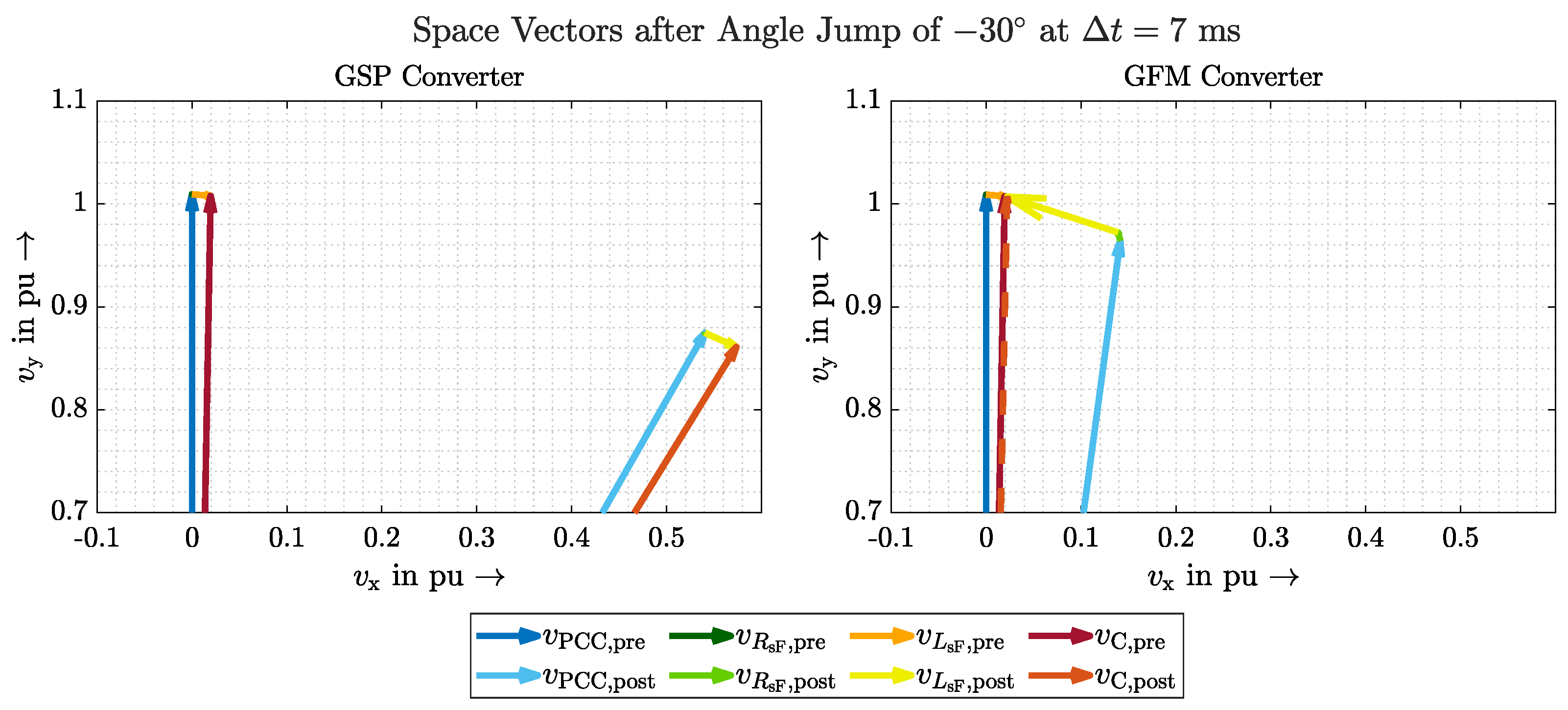
3.4. Space Vectors

A frequently used representation to show the inherent current or voltage source behaviour is space vector diagrams. They are often created as qualitative sketches, but in the following, the actually measured quantities are shown.

Figure 18 compares the space vector of the grid and converter voltages before and after an angle jump of the GSP and GFM converter.

Since the current is inherently kept constant by the GSP converter, the converter voltage must make the same angular jump as the grid voltage. This is clearly visible in the results. The GFM converter, on the other hand, keeps the voltage constant. The rotating xy reference frame also shows this characteristic well. The result is that the current adapts, which is evident from the changing voltage over the filter impedance. In particular, the voltage over the inductance grows rapidly because it is proportional to the change in the current. This stabilises the grid voltage and the angle jump at the selected time is much smaller than with the GSP control.

The same visualisation is used for the amplitude jump in Figure 19. As the results of the angle jump suggest, the converter voltage as well as the grid voltage in the GSP model jumps immediately by the set −0.05 pu. Since the synchronisation of the GVFM control used has the same inertia for amplitude jumps as for angle jumps, the space vector of the converter voltage also remains constant here. The stabilisation of the grid voltage and the filter voltage as a link are also evident here.

As mentioned above, this type of stabilisation and voltage stiffness is also possible in applications where no inherent active power can be provided. This type of analysis is therefore particularly suitable in these cases.

3.5. Locus Curves

While the space vectors give a good visualisation of the voltages, they only show an image at a given time. Therefore, the values of the grid and converter voltage are shown below as a function of time as a locus curve. Figure 20 shows the locus curves for the amplitude jump with interpolation points every $1\mathrm{ms}$ from 0 to $70\mathrm{ms}$. The interpolation points are marked in colour and can be assigned to the respective time with the colour bar on the right-hand side of the diagram.

This observation shows well that the amplitude of the voltages in the GSP control drops by 0.05 pu in the first 3 to 4 ms. After that, the $Q\left(V\right)$ droop is able to control the voltage and increase it again. The trajectory of the converter voltage follows that of the grid voltage very closely during the entire duration.

The converter voltage of the GFM converter, on the other hand, shows the inertia of the control. An inherent drop is not present at all and throughout the investigation, it runs smoothly and evenly. This stabilises the grid voltage, which initially drops rapidly but is immediately stopped by the converter voltage, which explains the loop in the grid voltage.

This behaviour is fundamentally different from that of the GSP converter and cannot be achieved even by higher-level controllers in the GVFL control, as these cannot become active in such a short period of time. Therefore, this and the previous presentation allow a clear identification of the control principle to be made without knowing how it is implemented. What is quickly apparent from the results can also be made verifiable through hard criteria.

3.6. Comparison of Different GVFM Controls

A requirement for a general definition of GVFM behaviour is that the behaviour of different GVFM controls can be classified together. Therefore, in the following, the behaviour of the VSM from Section 2.2.3 is compared with the control from Section 2.2.2, which is used for the previous results. Hence, the frequency behaviour for a load change is compared in Figure 21.

The results show that with the selected parameters, there is no difference in such a scenario. The influence on the grid frequency is identical both inherently and when stationary. In this case, however, it was decided not to activate an upper-level primary control. Since the implementation of a change in the reference values is solved with two different concepts, this does not allow for a good comparison. However, the native inertia of the control can be parameterised identically, which proves that the methods can be grouped together in this respect.

However, it has already been mentioned that in the chosen implementation, this only applies to the inertia for angle and/or frequency changes. In the explanation of the VSM control used, it was already pointed out that the control of the amplitude of the voltage has no inertia. To clarify this, the space vectors of the VSM control are shown in Figure 22 for an angle jump.

While the angle of the converter voltage also remains constant, as with the other GVFM control, the amplitude drops to the value of the grid voltage. This observation proves exactly what was described above. The conclusion for the explicit control method can be to rethink the RPC of the VSM control used and equip it with the same inertia as the APC. In terms of a general definition, however, this aspect must also be taken into account.

3.7. Variation in Primary Control Dynamics

A common mistake when evaluating converter behaviour is to associate virtual inertia with fast primary control. Although some of the results of this work have already shown that there are evident differences in instantaneous behaviour, this section will focus on the influence of different dynamics of the primary control.

The primary control, which is used in all models, is structured as follows: Deviations of the frequency f from the nominal frequency $f_{\mathrm{n}}$ are measured and filtered via a PT1 controller with the parameters $D_{fp}$ and ${\tau }_{fp}$. The determined adjustment is carried out via $\Delta p_{\mathrm{D}}\left(f\right)$. Equations (15) show this.

$$p^{★}=p_0^{★}+\Delta p_{\mathrm{D}}\left(f\right)$$

(15a)

$${\displaystyle \frac{d\Delta p_{\mathrm{D}}}{dt}}={\displaystyle \frac{1}{{\tau }_{fp}}}\left({\displaystyle \frac{p_{\max }}{D_{fp}}}(1-{\displaystyle \frac{f}{f_{\mathrm{n}}}})-\Delta p_{\mathrm{D}}\right)$$

(15b)

In the case of the GVFL control, f in Equation (15) is equal to the measured frequency $f_{\mathrm{PLL}}$. With the GVFM control, $f=f_{\mathrm{sync}}$ applies. The time constant ${\tau }_{fp}$ determines the dynamics of the control. Thus, Figure 23 shows the results of an angle jump for different values of ${\tau }_{fp}$.

It can be seen that dynamising the primary control of the GSP converter does not lead to greater inertia, as the angle jump is not delayed in any of the cases. Furthermore, it becomes clear that instabilities occur at high dynamics. This is not a new observation. In [34], for example, it could be shown that these instabilities are reached particularly quickly in weak grids or with a fast primary control. The results of the GFM converter also show that the inertia is not increased by a smaller ${\tau }_{fp}$. Thus, it can be concluded that a faster primary control cannot contribute to the virtual inertia of a converter—on the contrary, it can even cause or intensify instabilities when operated with a GVFL control.

3.8. Variation in Grid-Voltage-Forming Converter Inertia

However, by adjusting the dynamics of the synchronisation—or in the case of VSM, by changing the set inertia constant H—the inertia of converters with a GVFM control principle can be changed. This possibility offers another degree of freedom in contrast to the actual synchronous machine, whose inertia is determined by its physics and cannot be adjusted. Therefore, the following results explain the effect that changing the inertia of the control has on the grid behaviour of the system. To avoid the results being overlaid by the effect of the primary control, the GSB model is chosen in the following results.

Figure 24 shows the frequency deviation and its derivative in case of a load change. The set converter inertia $H_{\mathrm{C}}$ is altered between 60% and 140%.

It is clearly visible that a high inertia dampens the frequency deviation. This results in both a lower frequency nadir and a smaller RoCoF. However, it can be observed that the initial value of the frequency derivative is not related to the inertia. It can be assumed that in other network configurations, other results may be obtained if the maximum of the RoCoF is reached immediately.

A more reproducible scenario is therefore a defined angle or amplitude jump. Results for the resulting amplitude at the amplitude jump are plotted in Figure 25.

These results give a good representation of the dynamics of the synchronisation delay characteristics. If the set inertia is low, for example, because no high compensating currents are desired, the voltage drop is faster and has an overshoot. With higher dynamics, the steady-state value is reached later and without overshoot. This characteristic corresponds to other delay phenomena and could be compared with the results of a second-order delay. However, the requirement for this is that the amplitude is controlled with inertia, as already described in Section 3.6.

If the used GVFM control only controls the voltage angle with inertia—as the used VSM control does—the same analysis is carried out for an angle jump. The resulting angle of this investigation is shown in Figure 26.

These results illustrate that the same synchronisation with the same parameters applies to both amplitude and phase for the control used. Thus, the almost identical results are obtained. Despite the complex implementation of the control principles in their respective environments, some characteristic features can be identified that describe the converter behaviour well. This could help in the development of generic models of converters with GVFM controls.

3.9. Inertia Measurement

As described in Section 2.4, it is possible to measure the aggregated system inertia in grids that are dominated by the behaviour of synchronous machines. As Equation (14) shows, only the $df/dt$ has to be measured in the simulation environment used since the remaining variables and also the time of the load change are known. However, this is also where the difficulty can be found. Idealised, a change in the setpoint $p_{\mathrm{G}}^{★}$ would be specified for the grid equivalent used. This results in a frequency change from which the set inertia can be measured very precisely. In this case, however, the converter could not contribute its own virtual inertia. For this, the load change must be caused externally. However, this results in slight oscillations in the derivative of the frequency immediately after the load change. Figure 27 shows this phenomenon. The ideal, internal change described is compared with the more realistic, external change.

The results show that apart from the initial oscillations, the effect of the realistic load change matches the ideal effect very well. Nevertheless, since the initial, respectively, maximum value is decisive for the calculation of H, the results are inaccurate. What has become clear from the results in Section 3.2, however, is that the control used must have at least a qualitative influence on the RoCoF and thus also on the calculated $H_{\mathrm{calc}}$. Therefore, the calculation was carried out, although the inaccuracy of the results must be taken into account. For reference, instead of the set $H_{\mathrm{G}}=4.5\mathrm{s}$, a value of $H_{\mathrm{calc}}=4.23\mathrm{s}$ was measured without a converter. The values of the calculated inertia for the different converter behaviours are shown in Figure 28.

Without discussing the exact values, it is clearly visible that a GVFM control increases the value of the measured inertia. This also coincides with the results from Section 3.2 concerning the RoCoF. The GVFL control, on the other hand, is not able to improve the value; in this investigation, it even worsens it. Taking into account the mentioned inaccuracy, it can at least be stated that a GVFL control, in contrast to the GVFM control, does not improve the inertia of the system.

As described above, it is possible to adjust the set inertia of the GVFM control. It can be assumed that a higher set inertia is also expressed in a higher measured system inertia. This hypothesis was tested in a further investigation, the results of which are shown in Figure 29.

The assumption made can be confirmed by the results. Even if the relation between the adjusted converter inertia $H_{\mathrm{C}}$ and the measured system inertia $H_{\mathrm{calc}}$ is not linearly proportional to each other, the desired effect can be observed. A difference can also be detected between GFM and GSB converters. This would hint that the primary control combined with the GVFM control results in an improvement of the inertia. However, this conclusion is not necessarily correct due to the described difficulties in the measurement and the influence of the grid topology design on the results.

4. Discussion

The purpose of this work is to investigate which test environment is suitable for which proof with regard to converter behaviour. Three reference scenarios are tested for this purpose: load switching with a grid equivalent with synchronous machine behaviour, an amplitude jump, and an angle jump—each on a rigid voltage source with grid impedance. Aside from the question of which effects can be proven with which investigation, it is also important to mention how complex the models are and how reproducible the results are. These aspects are also relevant for a standardised test procedure.

Table 3. Comparison of the used reference scenarios.

	Load Change	Amplitude Jump	Angle Jump
Complexity of the model	Medium	Very low	Very low
Reproducibility of the results	Intermediate	Very easy	Very easy
Realism	High	Low	Very low
Proof of $\mathit{P}\left(\mathit{f}\right)$	✓	x	x
Proof of $\mathit{Q}\left(\mathit{V}\right)$	(✓)	✓	x
Proof of GVFM control principle	✓	✓1	✓2

¹ Voltage amplitude control needs to feature inertia. ² Size of the angle jump needs to consider available energy and current limits.

shows a comparison of the criteria mentioned.

The grid model for the load change is disclosed and explained in this work and it can thus certainly be reproduced. Yet, many simulation programmes already offer a voltage source with which amplitude and angle jumps can be simulated. This means that the effort required to simulate it is minimal. There are also fewer variables that can influence the results. This makes it easier to reproduce outcomes. However, load switching offers the highest realism, while a pure amplitude jump is rare and a pure angle jump without frequency change is impossible in the real grid.

In addition, only the load change can prove whether a $P\left(f\right)$ control is active. A $Q\left(V\right)$ control, on the other hand, can only be verified with an amplitude jump or a load change with a high reactive power, while it has no influence on the angle jump at all.

In general, all scenarios are suitable in this work to determine clear differences between GVFM and GVFL and thus to prove GVFM’s behaviour. A requirement for the amplitude jump, however, is a delayed control of the voltage amplitude, which is not given in the VSM model discussed, for example. The angle jump, on the other hand, must be designed in such a way that the available energy reserves are taken into account and that the current limits are not exceeded. This would force the converter to limit the current and perhaps give up stabilising the grid through inertia. How exactly to define the desired behaviour and prioritisation of a GVFM control in such a case should be the subject of further research.

5. Conclusions

This work uses simple simulations to show the grid behaviour of different converter models. No internal measured variables are used, but only measurements that would also be possible with protected simulation models from manufacturers or even in laboratory measurements. The results clearly show the differences in grid behaviour as well as their origin and the advantages of a GVFM control. Additionally, it is illustrated that there are possibilities to set a definition for GVFM controls based solely on the criterion of grid behaviour. The three tested reference scenarios are suitable for this purpose: a load change at a realistic grid replica and an amplitude as well as an angle jump at a rigid voltage source. The advantages and disadvantages of these models are also compared.

Furthermore, it is shown how the aggregated system inertia can be measured in the grid model. The inaccuracies of this measurement are discussed in detail, which is why the inertia is not necessarily suitable as a measure of grid strength in converter-dominated grids. Nevertheless, it is shown that it has at least qualitative significance and can therefore also serve as a criterion for requirements for converter systems.

In addition, outlooks are given on how GVFM’s behaviour could be understood in general and reproduced in generic models. This aspect, as well as the further development of definition and testing procedures for GVFM behaviour, should be the subject of future research.

References

1. H2020 MIGRATE Project. D1.1—Current and Arising Issues Caused by Increasing Power Electronics Penetration. Available online: https://www.h2020-migrate.eu/_Resources/Persistent/dacdf9db7dffbeb16071037ea26c2f20aac6ed46/D1.1%20summary%20and%20questionnaire%20for%20external%20stakeholders_vf.pdf (accessed on 12 September 2023).
2. Ulbig, A.; Borsche, T.S.; Andersson, G. Impact of Low Rotational Inertia on Power System Stability and Operation. Ifac Proc. Vol. 2014, 47, 7290–7297. [Google Scholar] [CrossRef]
3. Tielens, P.; van Hertem, D. The relevance of inertia in power systems. Renew. Sustain. Energy Rev. 2016, 55, 999–1009. [Google Scholar] [CrossRef]
4. Matevosyan, J.; Vital, V.; O’Sullivan, J.; Quint, R.; Badrzadeh, B.; Prevost, T.; Quitmann, E.; Ramasubramanian, D.; Urdal, H.; Achilles, S.; et al. Grid-Forming Inverters: Are They the Key for High Renewable Penetration? IEEE Power Energy Mag. 2019, 17, 89–98. [Google Scholar] [CrossRef]
5. NERC. White Paper: Grid Forming Functional Specifications for BPS-Connected Battery Energy Storage Systems. NERC. Available online: https://www.nerc.com/comm/RSTC_Reliability_Guidelines/White_Paper_GFM_Functional_Specification.pdf (accessed on 25 October 2023).
6. Shakerighadi, B.; Johansson, N.; Eriksson, R.; Mitra, P.; Bolzoni, A.; Clark, A.; Nee, H.P. An overview of stability challenges for power–electronic–dominated power systems: The grid—Forming approach. IET Gener. Transm. Distrib. 2023, 17, 284–306. [Google Scholar] [CrossRef]
7. Weise, B.; Korai, A.; Constantin, A. Comparison of Selected Grid-Forming Converter Control Strategies for Use in Power Electronic Dominated Power Systems. In Proceedings of the 18th Wind Integration Workshop, Dublin, Ireland, 16–18 October 2019. [Google Scholar]
8. Rocabert, J.; Luna, A.; Blaabjerg, F.; Rodríguez, P. Control of Power Converters in AC Microgrids. IEEE Trans. Power Electron. 2012, 27, 4734–4749. [Google Scholar] [CrossRef]
9. Struwe, J.; Wrede, H.; Vennegeerts, H. System Characteristics of Grid-Forming and Grid-Following Converter Systems. In Proceedings of the 2023 25th European Conference on Power Electronics and Applications (EPE’23 ECCE Europe), Aalborg, Denmark, 4–8 September 2023; pp. 1–9. [Google Scholar] [CrossRef]
10. H2020 MIGRATE Project. D3.6—Requirement Guidelines for Operating a Grid with 100 Power Electronic Devices. Available online: https://www.h2020-migrate.eu/_Resources/Persistent/1bb0f89024e41a85bf94f1ec7ee6f8d7c34bc29a/D3.6%20-%20Requirement%20guidelines%20for%20operating%20a%20grid%20with%20100%20power%20electronic%20devices.pdf (accessed on 12 September 2023).
11. UNIFI. Grid-forming Inverter Technology Specifications: A Review of Research Reports & Roadmaps. Available online: https://drive.google.com/file/d/1YRwF1mNH2pA-WKlQ_HVbEYCQy4iWsAB_/view (accessed on 25 October 2023).
12. Winter, P. Netzspannungsbildende und -folgende Umrichtersysteme am elektrischen Energieversorgungsnetz: Regelungsentwurf, Analyse und Stabilitätsbetrachtung. Ph.D. Thesis, University of Duisburg-Essen, Essen, Germany, 2021. [Google Scholar] [CrossRef]
13. Unruh, P.; Nuschke, M.; Strauß, P.; Welck, F. Overview on Grid-Forming Inverter Control Methods. Energies 2020, 13, 2589. [Google Scholar] [CrossRef]
14. Rosso, R.; Wang, X.; Liserre, M.; Lu, X.; Engelken, S. Grid-Forming Converters: Control Approaches, Grid-Synchronization, and Future Trends—A Review. IEEE Open J. Ind. Appl. 2021, 2, 93–109. [Google Scholar] [CrossRef]
15. Blasko, V.; Kaura, V. A new mathematical model and control of a three-phase AC-DC voltage source converter. IEEE Trans. Power Electron. 1997, 12, 116–123. [Google Scholar] [CrossRef]
16. Timbus, A.; Liserre, M.; Teodorescu, R.; Rodriguez, P.; Blaabjerg, F. Evaluation of Current Controllers for Distributed Power Generation Systems. IEEE Trans. Power Electron. 2009, 24, 654–664. [Google Scholar] [CrossRef]
17. Vasquez, J.C.; Guerrero, J.M.; Luna, A.; Rodriguez, P.; Teodorescu, R. Adaptive Droop Control Applied to Voltage-Source Inverters Operating in Grid-Connected and Islanded Modes. IEEE Trans. Ind. Electron. 2009, 56, 4088–4096. [Google Scholar] [CrossRef]
18. D’Arco, S.; Suul, J.A. Equivalence of Virtual Synchronous Machines and Frequency-Droops for Converter-Based MicroGrids. IEEE Trans. Smart Grid 2014, 5, 394–395. [Google Scholar] [CrossRef]
19. Markovic, U.; Vorwerk, J.; Aristidou, P.; Hug, G. Stability Analysis of Converter Control Modes in Low-Inertia Power Systems. In Proceedings of the 2018 IEEE PES Innovative Smart Grid Technologies Conference Europe (ISGT-Europe), Sarajevo, Bosnia and Herzegovina, 21–25 October 2018; pp. 1–6. [Google Scholar] [CrossRef]
20. Strunz, K.; Almunem, K.; Wulkow, C.; Kuschke, M.; Valescudero, M.; Guillaud, X. Enabling 100 % Renewable Power Systems Through Power Electronic Grid-Forming Converter and Control: System Integration for Security, Stability, and Application to Europe. Proc. IEEE 2022, 11, 891–915. [Google Scholar] [CrossRef]
21. D’Arco, S.; Suul, J.A.; Fosso, O.B. Small-signal modelling and parametric sensitivity of a Virtual Synchronous Machine. In Proceedings of the 2014 Power Systems Computation Conference, Wroclaw, Poland, 18–22 August 2014; pp. 394–395. [Google Scholar] [CrossRef]
22. Winter, P.; Wrede, H.; Struwe, J.; Cajigal, J. Control Design and Analysis for Grid-Connected Converter Systems with Island Ability. In Proceedings of the 2021 IEEE Green Technologies Conference (GreenTech), Denver, CO, USA, 7–9 April 2021; pp. 364–371. [Google Scholar] [CrossRef]
23. Winter, P.; Cajigal-Nunez, J.M.; Wrede, H.; Struwe, J. Analysis of an sDFT-PLL for Grid-Forming Control Methods. In Proceedings of the 2020 IEEE 9th International Power Electronics and Motion Control Conference (IPEMC2020-ECCE Asia), Nanjing, China, 29 November–2 December 2020; pp. 323–330. [Google Scholar] [CrossRef]
24. Kundur, P. Power System Stability and Control, xxiii ed.; The EPRI Power System Engineering Series; McGraw-Hill: New York, NY, USA, 1994. [Google Scholar]
25. ENTSO-E. High Penetration of Power Electronic Interfaced Power Sources (HPoPEIPS): ENTSO-E Guidance Document for National Implementation for Network Codes on Grid Connection. Available online: https://consultations.entsoe.eu/system-development/entso-e-connection-codes-implementation-guidance-d-3/user_uploads/igd-high-penetration-of-power-electronic-interfaced-power-sources.pdf (accessed on 25 October 2023).
26. Inoue, T.; Taniguchi, H.; Ikeguchi, Y.; Yoshida, K. Estimation of power system inertia constant and capacity of spinning-reserve support generators using measured frequency transients. IEEE Trans. Power Syst. 1997, 12, 136–143. [Google Scholar] [CrossRef]
27. Ashton, P.M.; Saunders, C.S.; Taylor, G.A.; Carter, A.M.; Bradley, M.E. Inertia Estimation of the GB Power System Using Synchrophasor Measurements. IEEE Trans. Power Syst. 2015, 30, 701–709. [Google Scholar] [CrossRef]
28. Heylen, E.; Teng, F.; Strbac, G. Challenges and opportunities of inertia estimation and forecasting in low-inertia power systems. Renew. Sustain. Energy Rev. 2021, 147, 111176. [Google Scholar] [CrossRef]
29. Kontis, E.O.; Pasiopoulou, I.D.; Kirykos, D.A.; Papadopoulos, T.A.; Papagiannis, G.K. Estimation of power system inertia: A Comparative assessment of measurement-Based techniques. Electr. Power Syst. Res. 2021, 196, 107250. [Google Scholar] [CrossRef]
30. Dimoulias, S.C.; Kontis, E.O.; Papagiannis, G.K. Inertia Estimation of Synchronous Devices: Review of Available Techniques and Comparative Assessment of Conventional Measurement-Based Approaches. Energies 2022, 15, 7767. [Google Scholar] [CrossRef]
31. Ackermann, T.; Prevost, T.; Vittal, V.; Roscoe, A.J.; Matevosyan, J.; Miller, N. Paving the Way: A Future Without Inertia Is Closer Than You Think. IEEE Power Energy Mag. 2017, 15, 61–69. [Google Scholar] [CrossRef]
32. Wang, B.; Sun, H.; Li, W.; Yang, C.; Wei, W.; Zhao, B.; Xu, S. Power system inertia estimation method based on maximum frequency deviation. IET Renew. Power Gener. 2022, 16, 622–633. [Google Scholar] [CrossRef]
33. Sajadi, A.; Rañola, J.A.; Kenyon, R.W.; Hodge, B.M.; Mather, B. Dynamics and Stability of Power Systems With High Shares of Grid-Following Inverter-Based Resources: A Tutorial. IEEE Access 2023, 11, 29591–29613. [Google Scholar] [CrossRef]
34. Winter, P.; Struwe, J.; Cajigal, J.; Wrede, H. Stability Margins of Grid-Supporting Converters. In Proceedings of the 2021 IEEE Green Technologies Conference (GreenTech), Denver, CO, USA, 7–9 April 2021; pp. 387–394. [Google Scholar] [CrossRef]
Figure 1. Grid topology with the converter connected via an LC filter and a transformer to the grid.
Energies 16 07357 g001
Figure 2. Calculation of the converter and filter voltages with differential equations.
Energies 16 07357 g002
Figure 3. Control of the grid equivalent resembling a synchronous machine.
Energies 16 07357 g003
Figure 4. Control of the rigid voltage source enabling amplitude and angel jumps.
Energies 16 07357 g004
Figure 5. Control scheme of the current control.
Energies 16 07357 g005
Figure 6. Control scheme of the grid-voltage-forming control.
Energies 16 07357 g006
Figure 7. Magnitude and angle synchronisation of the grid-voltage-forming control.
Energies 16 07357 g007
Figure 8. Frequency synchronisation of the grid-voltage-forming control.
Energies 16 07357 g008
Figure 9. Control scheme of the virtual synchronous machine.
Energies 16 07357 g009
Figure 10. Active power control of the virtual synchronous machine.
Energies 16 07357 g010
Figure 11. Reactive power control of the virtual synchronous machine.
Energies 16 07357 g011
Figure 12. Rotating xy reference frame.
Energies 16 07357 g012
Figure 13. Validation of the voltage and filter voltages calculation.
Energies 16 07357 g013
Figure 14. Frequency deviation and derivative of different converter behaviours for a load change.
Energies 16 07357 g014
Figure 15. Amplitude and angle of grid and converter voltages of different converter behaviours for a load change.
Energies 16 07357 g015
Figure 16. Angle of grid and converter voltages of different converter behaviours for an angle jump.
Energies 16 07357 g016
Figure 17. Amplitude of grid and converter voltages of different converter behaviours for an amplitude jump.
Energies 16 07357 g017
Figure 18. Space vectors of GSP and GFM converter for an angle jump.
Energies 16 07357 g018
Figure 19. Space vectors of GSP and GFM converter for an amplitude jump.
Energies 16 07357 g019
Figure 20. Locus curve of grid and converter voltages of GSP and GFM control for an amplitude jump.
Energies 16 07357 g020
Figure 21. Frequency deviation and derivative of different GVFM controls after a load change.
Energies 16 07357 g021
Figure 22. Space vectors of virtual synchronous machine after a load change.
Energies 16 07357 g022
Figure 23. Angle of converter voltage of GSP and GFM converter for different dynamics.
Energies 16 07357 g023
Figure 24. Frequency deviation and derivative of GSB control for different converter inertia after a load change.
Energies 16 07357 g024
Figure 25. Converter voltage amplitude of GSB control for different converter inertia after an amplitude jump.
Energies 16 07357 g025
Figure 26. Converter voltage angle of GSB control for different converter inertia after an angle jump.
Energies 16 07357 g026
Figure 27. Frequency deviation and derivative for an ideal and realistic load change.
Energies 16 07357 g027
Figure 28. Calculated system inertia for different converter controls.
Energies 16 07357 g028
Figure 29. Calculated system inertia for GSB and GFM converter for different converter inertia.
Energies 16 07357 g029