Abstract
Wireless energy harvesting (EH) communication has long been considered a sustainable networking solution. However, it has been limited in efficiency, which has been a major obstacle. Recently, strategies such as energy relaying and borrowing have been explored to overcome these difficulties and provide long-range wireless sensor connectivity. In this article, we examine the reliability of a wireless-powered communication network by maximizing the net bit rate. To accomplish our goal, we focus on enhancing the performance of hybrid access points and information sources by optimizing their transmit power. Additionally, we aim to maximize the use of harvested energy, by using energy-harvesting relays for both information transmission and energy relaying. However, this optimization problem is complex, as it involves non-convex variables and requires combinatorial relay selection indicator optimization for decode and forward (DF) relaying. To simplify this problem, we utilize the Markov decision process and deep reinforcement learning framework based on the deep deterministic policy gradient algorithm. This approach enables us to tackle this non-tractable problem, which conventional convex optimization techniques would have difficulty solving in complex problem environments. The proposed algorithm significantly improved the end-to-end net bit rate of the smart energy borrowing and relaying EH system by and compared to the benchmark algorithm based on borrowing energy with an adaptive reward for Quadrature Phase Shift Keying, 8-PSK, and 16-Quadrature amplitude modulation schemes, respectively.
1. Introduction
The deployment of ultra-low-power electronic sensors has increased significantly with the advanced wireless communication networks [1]. These sensors are used for various data collection and signal processing applications of the Internet of Things (IoT) domain [2]. However, the lifetime of the IoT networks is limited by the battery constraints of the individual sensor devices. To address this issue, dedicated radio frequency energy transfer (RF-ET) ensures uninterrupted long-duration network operation by providing controllable on-demand energy replenishment of sensor devices [3], which includes long-range beamforming capabilities for energy harvesting (EH), joint energy, and information transfer provisioning over the same signal [4]. This introduces a research paradigm on wireless-powered communication networks (WPCN), in which the uplink information transfer (IT) is governed by downlink ET from the hybrid access point (HAP).
The RF-EH system can operate independently in remote and harsh locations, but it has some limitations. These include low energy sensitivity, low rectification efficiency at lower input power, high attenuation due to path loss, and energy dispersion loss [5]. Additionally, the energy harvested from ambient sources cannot be accurately predicted dynamically because the channel conditions are constantly changing [6]. Therefore, it is necessary to have a backup power supply, such as a power grid (PG), to facilitate energy cooperation. This secondary power supply can efficiently handle energy transactions when EH devices require additional power for uninterrupted WPCN operation. This paper investigates the artificial intelligence (AI) enabled smart energy sharing and relaying in cooperative WPCN to enhance the end-to-end system performance.
1.1. Related Works
Several studies, including those referenced in citations [7,8,9,10,11,12,13], have explored implementing autonomous cooperative energy harvesting (EH) techniques with unknown channel gains. These techniques involve energy-constrained sensor devices transmitting information using harvested energy in wireless power transfer networks (WPCN). For instance, one study proposed an optimization model in [7] to maximize two-hop radio frequency energy transfer efficiency with optimal relay placement. In [8], the authors maximized the overall bit rate by optimizing time and power allocation for downlink energy transfer and uplink information transfer and relaying. Another study by Chen et al. in [9] approximated the average throughput for wireless-powered cooperative networks using the harvest-then-cooperate protocol. In addition to fixed relaying approaches in [8,9], an adaptive transmission protocol in [10] dynamically determines whether the information source (IS) should access the point (AP) directly or cooperatively with relays based on estimated channel state information (CSI). Beamforming optimization was performed in [11] to maximize received power for evaluating the performance of relay-assisted schemes under EH efficiency constraints. In [12], a cooperative relaying system was developed to improve the quality of experience (QoE) for cell-edge users. In [13], Wei et al. proposed wireless power transfer (WPT) to enhance spectral efficiency (SE) by jointly adjusting time slot duration, subcarriers, and the transmit power of the source and relay. However, the harvested energy from WPT at sensor device batteries cannot transmit data over long distances. Therefore, energy cooperation and sharing strategies are necessary to overcome dynamic green energy arrival conditions for perpetual WPCN operation.
In network optimization, ref. [14] proposed a method to minimize network delay through simplified energy management and conservation constraints for fixed data and energy routing topologies. Meanwhile, ref. [15] explored various energy-sharing mechanisms among multiple EH devices within the network. When data transmission is possible, but there is insufficient energy in the device battery, external energy supply from nearby secondary power sources must be considered. Ref. [16] addressed this issue by examining the external energy supply provided by PG to EH devices in WPCN. In contrast, ref. [17] proposed that EH devices borrow energy from PG for information transmission and return it with additional interest as a reward. Sun et al. developed a schedule [18,19,20] to maximize system throughput through energy borrowing and returning. However, these approaches rely on predefined statistical parameters and dynamics, whereas in reality, channel gains and harvested energy are subject to random variation. Therefore, a decision-making deep reinforcement learning (DRL) algorithm is needed to determine current network parameters based on previously gained knowledge of the environment.
Wireless network management has recently seen an increase in deep reinforcement learning (DRL) use as part of machine learning (ML) due to its decision-making capabilities through a trial-and-error approach. The sophisticated combination of neural networks (NNs) in DRL makes it ideal for handling complex situations with high-dimensional problems. The authors of [21] developed an NN model to extract key rates with high reliability, considerable tightness, and great efficiency. Qie et al. [22] used DRL based on the deep deterministic policy gradient (DDPG) algorithm to develop an optimal energy management strategy for an EH wireless network. Resource allocation policies were also developed using DRL in [23] to maximize achievable throughput, considering EH, causal information of the battery state, and channel gains. DRL based on borrowing energy with an adaptive reward (BEAR) algorithm was proposed in [24] to optimize energy borrowing from a secondary power source and efficient data transfer utilizing harvested energy. In [25], cooperative communications with adaptive relay selection in a wireless sensor network were investigated as a Markov decision process (MDP), and deep-Q-network (DQN) was proposed to evaluate network performance. DRL based on the actor-critic method was used in [26,27] to maximize the energy efficiency (EE) of a heterogeneous network for optimal user scheduling and resource allocation. However, the impact of energy scheduling and transmit power allocation of IS maximizing the transmission rate of an energy borrowing and relaying aided WPCN is still a research gap, needs to be explored.
1.2. Motivation and Key Contributions
In current EH cooperative relaying techniques for WPCN, such as those mentioned in references [10,11,12,13], having complete knowledge of the CSI at the receiver is necessary. However, such simplified channel models fail to account for the dynamic communication environment, which is crucial for optimizing resource allocation and analyzing system performance. Alternative approaches, like energy scheduling and management methods, have been adopted in references [15,16,17,18], which assume a practical probability distribution model for energy arrival. However, these methods do not consider optimal power allocation, energy borrowing, and returning schedules for harvested energy relaying for IT. Only the authors of reference [21,23,24] have considered a practical EH channel model, where a single EH relay wirelessly transfers energy to the IS. However, this model does not apply to multiple EH relay-assisted WPCN, where maximizing throughput and minimizing transmission delay are essential. Our article addresses these issues by exploring the RF-powered joint information and energy relaying (JIER) protocol for WPCN, which efficiently allocates resources to maximize system reliability. Specifically, we consider an EH-HAP that effectively manages energy transactions with the PG and transmits RF energy to the IS through multiple EH relays. It then receives information from the source via uplink DF-relay-assisted channels. This timely investigation focuses on maximizing the efficacy of EH in WPCN by optimally utilising the available energy resources by enabling intelligent energy relaying and borrowing. Our specific contribution is four-fold, which can be summarized as follows:
- Considering a novel smart energy borrowing and relaying-enabled EH communication scenario, we investigate the end-to-end net bit rate maximization problem in WPCN. Here, we jointly optimize the transmit power of HAP and IS, fractions of harvested energy transmitted by the relays, and the relay selection indicators for DF relaying within the operational time.
- We decompose the formulated problem into multi-period decision-making steps using MDP. Specifically, we propose a nontrivial transformation where the state represents the current onboard battery energy level and the instantaneous channel gains. In contrast, the corresponding action indicates the transmit power allocations. Since HAP selects the relay based on the maximum achievable signal-to-noise ratio (SNR) among all the relays for receiving the information, the instantaneous transmission rate attained by HAP is treated as an immediate reward.
- We observed that the initial joint optimization problem was analytically intractable to be solved using traditional convex optimization techniques due to the realistic parameter settings of complex communication environments. Therefore, we suggest a DRL framework using the DDPG algorithm to train the DNN model, enabling the system to discover the best policy in an unfamiliar communication environment. The proposed approach determines the current policy using the Q-value for all state-action pairs. Additionally, we have examined the convergence and complexity of the proposed algorithm to improve the learning process.
- Our analysis is validated by the extensive simulation results, which offer valuable insights into the impact of key system parameters on optimal decision-making. Additionally, we compared the performance of various modulation schemes, including QPSK, 8-phase shift keying (PSK), and 16-quadrature amplitude modulation (QAM), that leverage the same algorithm. Our resource allocation technique improves the net bit rate of the system compared to the BEAR-based benchmark algorithm.
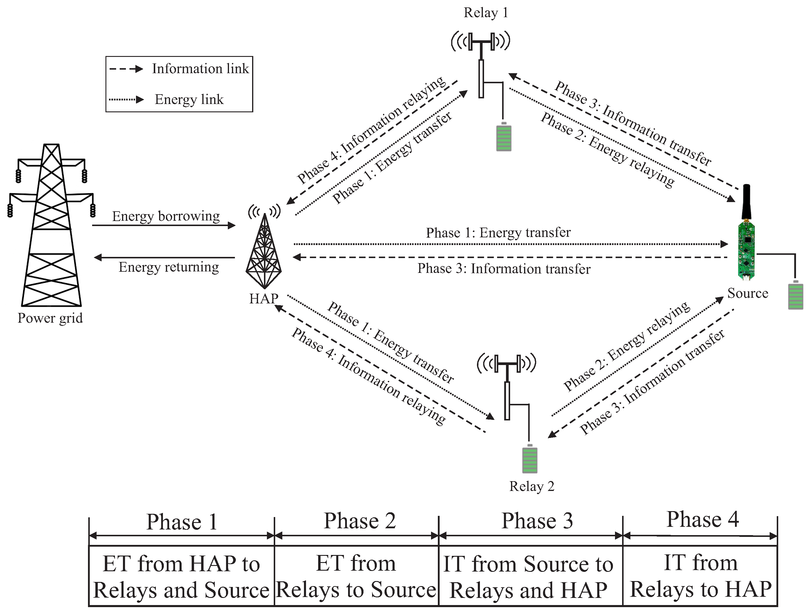
The rest of the article is organized as follows: Section 2 presents the system model of efficient WPCN (Figure 1). Section 3 elaborates on the mathematical formulation of our objective. Section 4 introduces the DRL approach and the proposed DDPG algorithm for resource allocation corresponding to the optimal policy. Section 5 gives insights into extensive simulation results for performance evaluation. Finally, Section 6 outlines the conclusion, where the list of references is located at the end of this article.
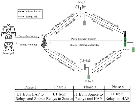
Figure 1.
System model of the WPCN.
We use bold letters to denote vector quantity; represents the magnitude of a complex quantity; stands for complementary error function; indicates a circularly symmetric complex Gaussian random variable with mean and variance ; is the expectation operator; and denotes the big-O notation.
2. System Model
Consider a JIER-assisted WPCN consisting of a PG and three types of transceiver modules such as a HAP, two RF-EH relays, and an IS, as depicted in Figure 1. Here, HAP is harvesting energy from ambient sources, such as RF power signals, and subsequently stores the harvested energy in its limited charge storage capable internal battery. We assume that IS can only harvest energy into its small-size battery storage from the RF energy transfer mode as it has no direct external energy supply. When IS accumulates sufficient energy, it can transmit information to relays and HAP. Furthermore, HAP can borrow the required energy from the PG while it faces the potential energy shortage for RF energy transmission towards relays and IS. To reduce PG’s additional burden, HAP returns the borrowed energy to PG along with interest based on the borrowing price, where no energy leakage is considered within the energy transmission deadline [28]. For ease of calculation, we subdivide the operational period into N equally spaced discrete time slots of duration each. Let, at the nth time slot, the battery energy level of HAP is and its harvested energy from the ambient sources is , where follows the Gaussian distribution of mean and variance . The channel gain coefficient for the communication link between source and destination at the nth time slot also follows the complex Gaussian distribution of mean and variance [29].
2.1. JIER Protocol
We consider that HAP can transfer energy to IS by the two RF-EH relays, i.e., and via full-duplex two-hops downlink channel and then IS transmits data to the HAP via uplink half-duplex decode and forward (DF) relaying channel. The entire protocol is divided into four phases as follows:
- Phase 1: Energy is harvested at , and the IS for time slots by the directly transmitted RF signals from the HAP.
- Phase 2: Energy is further harvested at the IS in th time slot by energy relaying from and , where the relays transmit a fraction of the harvested energy from phase 1. Let and be the fractions of the harvested energy transmitted by and , respectively.
- Phase 3: At the th time slot, the IS directly transmits information to , and the HAP using the harvested energy stored in its onboard battery.
- Phase 4: Finally, at Nth time slot, the information is transmitted to the HAP from or via DF relaying by utilizing the remaining harvested energy stored in the relays’ battery. The HAP receives information from a single relay at a time and selects that relay depending on the maximum achievable SNR among all the relays.
2.2. Energy Scheduling
The instantaneous battery energy level of the HAP depends on its current harvesting energy, energy borrowing, and returning of energy to PG, which can be calculated as [28]
where is the maximum battery capacity of HAP, represents the instantaneous borrowed energy from PG, denotes the returned energy to PG at nth time slot, and is the instantaneous transmit power of HAP.
2.2.1. Energy Borrowing
If HAP’s current energy level is less than its energy consumption at a slot while transmitting with the power of , HAP borrows the required energy from the PG, which can be expressed as [28]
2.2.2. Energy Returning
Since sometimes HAP borrows the required energy from PG according to (2), it has to be returned to PG along with the interest based on the borrowing price. Hence, HAP returns it by utilizing the harvested energy at future time slots, defined by [24]
where is the instantaneous excess energy, denotes the energy transfer efficiency from HAP to PG, and indicates the unreturned energy, which is defined at nth time slot as [24]
where is the excess returnable energy in the form of interest because of delay in returning the borrowed energy, and denotes the rate of interest. To restrict excessive energy borrowing, we set the upper bound of unreturned energy during the entire energy transmission process, expressed by .
2.3. RF Energy Harvesting
As we mentioned earlier in Section 2.1 that energy is harvested in and and IS during the first two phases, we employ a linear harvesting model in this case. According to this model, instantaneous stored harvested energies at , and IS are calculated as [29]
where is RF-EH efficiency, , , , , and are the instantaneous channel gains between the links of HAP to , HAP to , HAP to IS, to IS, and to IS respectively.
3. Problem Definition
3.1. DF Relay-Assisted Information Transfer
The performance metric of the proposed WPCN is defined as the instantaneous bit rate, which refers to the number of bits transmitted per unit of time over the communication channel. Various factors, including the modulation scheme, channel bandwidth, coding scheme, and the presence of any error correction or data compression techniques, influence the bit rate that can be expressed at nth time slot as [29]
where is the number of bits containing a symbol, represents the number of symbols in a packet, denotes the packet duration, and is the instantaneous end-to-end bit error rate (BER), which can be expressed for DF relaying system as [28]
where is the instantaneous transmit power of IS, and are the instantaneous transmit power of and respectively to relay the information toward HAP, is noise power received at , , and HAP. and are two modulation-related parameters whose values are provided in Table 1. Here, d stands for the particular constant that modulation index m determines in the nth time slot. Furthermore, as HAP receives information from a single relay at a time slot, we define relays and selection indicators at nth time slot respectively as

Table 1.
Different values of modulation parameters for the three considered schemes.
3.2. Optimization Formulation
To improve the reliability of the proposed WPCN, we maximize the end-to-end net bit rate from IS to HAP by finding the optimal transmit power of HAP and IS, fractions of harvested energy transmitted by relays, and relay selection indicator for DF relaying within the operational period. The associated optimization problem is formulated as follows:
Here, , , , and set the instantaneous boundary conditions for the HAP and IS’s transmit power, borrowing, and the returning energy of the HAP, respectively; implies that the unreturned energy of the HAP at the end of the operation has to be zero, but it should not exceed the certain threshold during the operation; specifies the fractions of harvested energy transmitted by the relays and ; and verifies the relay selection indicators.
The formulated problem is combinatorial because the fractions of the harvested energy transmitted by the relays at phase 2 are related to their transmit power at phase 4, which is also associated with HAP’s transmit power at phase 1. Furthermore, since the optimization problem is nontrivial, due to the nonlinear structure of the objective function and non-convex constraints, traditional convex optimization requires several approximation steps to obtain suboptimal solutions.In addition, the channel gain and energy arrival rate are unpredictable in a practical wireless communication environment. Hence, we propose a DRL model using the DDPG algorithm to maximize objective value, which also guarantees fast convergence.
4. DRL-Based Solution Methodology
The original optimization problem has multiple decision variables, making it combinatorial and originating several nonconvexity issues. Hence, we formulate an MDP-based DRL framework in which the system interacts with the unknown environment to learn the best decision-making policy for improving the objective value.
4.1. MDP Framework
A centralized controller executes the DRL framework while simultaneously observing PG, HAP, EH relays, and IS. As the current state of these network elements depends on the immediate past state value, the optimization problem can be simplified by an MDP-based sequential decision-making policy.
4.1.1. State Space
Since the transmit powers, fractions of harvested energy transmitted by relays, and relay selection depend on current channel gains, battery level, and harvested energy, the instantaneous state vector is defined as
where , , and are the instantaneous battery level of the relay , , and IS respectively, , , and are their respective maximum battery capacity.
4.1.2. Action Space
According to the decision-making policy, the values of the optimizing variables are determined. Therefore, these are characterized by the transmit power of HAP and IS, fractions of harvested energy transmitted by relays, and relay selection indicators at every instance. Hence, the instantaneous action vector is defined as:
4.1.3. Reward Evaluation
Since the reward defines the quality of an action taken at a particular state, the immediate reward function to maximize the objective value over the long term is expressed as an instantaneous end-to-end net bit rate
4.1.4. State Transition
It is the probability that the current state transits to the next state after taking a current action . In our model, channel gains and harvested energy are uncertain and must be learned during decision-making. As these decision variables mostly follow Gaussian distribution, we must estimate their distribution parameters, such as mean and variance, over the simulation episode to maximize the cumulative long-term reward. We define the instantaneous channel gain values and harvested energy according to their current distribution parameters as , , , , , and respectively. Depending on their values, battery levels at the next time slot are measured as
4.2. Decision-Making Policy
The system gathers information on the surrounding environment through interaction to obtain a sub-optimal decision-making policy. Initially, it does not know the properties of the communication environment. Therefore, it tentatively selects action at a given state, immediately receives reward, and obtains value for the current state-action pair. Then the current state is updated to the next state . Here, the expected mapping value between the current state and the following action can be mathematically represented by [29]
where denotes the discount factor, and represents a deterministic policy for the decision-making process.
Due to the difficulties of finding the gradient of the current policy , we model it as a Gaussian distribution with mean and standard deviation , where the policy distribution can be expressed as [27]
Since the maximum and minimum values of policy parameters lie within a range, we apply the hyperbolic tangent function to restrict its output between and 1, represented by [24]
where is the effective energy level, and is the feature vector of the current state . It contains two binary functions and such that, if the battery energy level exceeds its minimum value, and the battery energy level has achieved its maximum value respectively. Otherwise, they are set to zero for other cases. Since the standard deviation should be positive, it is modeled by a linear exponent as . This proposed Gaussian policy allocates transmit power at each time slot. In all but the N-th time slot within the last k time slots, the transmission power abides by a certain condition. This condition is put in place to guarantee that any energy that was borrowed is properly returned to the power grid and it can be expressed as follows:
This condition holds for a sufficient amount of energy can be returned to the PG efficiently, where k is proportional to and . Here plays a critical role in determining the margin due to variations in harvested energy.
4.3. Proposed DDPG Algorithm
DDPG is an RL framework that can handle the continuous state and action spaces based on policy and Q-value evaluation. It utilizes policy evaluation NN with parameter which takes the state vector as input and outputs corresponding action vector . Policy evaluation NN consists of an input layer of thirteen neurons, three successive hidden layers of , , and neurons, and an output layer of six neurons. As the normalized action vector can only be a positive value for a given positive value state vector, we apply the sigmoid activation function to better tune the policy NN model. After taking action at the current state , the immediate reward is generated and the current state is updated to the next state . Then, the sample data tuple is stored in the experience memory. During the reinforcement learning process, a data tuple consisting of the current state vector, action vector, reward resulting from the action, and the next state vector is stored in the experience memory. The Q-value evaluation neural network is trained using a batch of randomly selected samples from the experience memory. The neural network, denoted as with parameter , takes the state and action vectors as input and provides the state-action value as output. This neural network has an input layer comprising nineteen neurons, three hidden layers consisting of , , and neurons, respectively, and an output layer with a single neuron. As the desired output Q value is always a positive number, we apply the sigmoid activation function to tune the Q-value evaluation NN. The policy and Q-value target NNs, respectively represented by and with parameters and replicating the same structure as the policy and Q-value evaluation NNs respectively are applied to stabilize the training process. The parameter of the Q-value evaluation NN, , is updated by minimizing the temporal difference (TD) error loss, which is expressed as [21]:
where , the output of the Q-value target NN is calculated using the output of the policy target network as [21]:
where is the discount factor. The parameters of policy evaluation NN can be updated through the deterministic policy gradient method, which is given as [21]:
Finally, the parameters of the target NNs are updated slowly with respect to learning rate as [21]:
4.4. Implementation Details
Algorithm 1 implements the end-to-end net bit rate maximization in the proposed EH relay-assisted WPCN. In the beginning, the four NNs, namely, policy evaluation NN, policy target NN, Q-value evaluation NN, and Q-value target NN, are initialized with random weight vectors. Then, inside the main loop, policy evaluation NN takes the current state as input for each time slot and approximates the action value. In order to keep exploration, we add Gaussian noise of variance to the current action. After choosing the action, the current state updates to a new state and generates an immediate reward by (14). Then, the transition data set, consisting of the current state, action, reward, and the next state, is stored in experience memory to train the DRL model. When the filled memory length is greater than the batch size, randomly sample a mini-batch of transition data from memory, calculate the loss values, and update the parameters of policy and Q-value evaluation NNs by (24) and (22), respectively. Then, the algorithm updates the parameters of the target NNs by (25) and (26) and also updates the current state as the next state. Finally, the running episode is terminated when the system elapsed maximum operational time steps, and the obtained policy corresponding to the last episode makes optimal decision variables.
| Algorithm 1 DRL based on DDPG for end-to-end net bit rate maximization |
| Require: N, T, , , , , , , |
| Ensure: , , , , , , |
|
The centralized controller implements the proposed algorithm to train the above-mentioned NN configurations. The proposed algorithm’s computational complexity depends entirely on the defined NNs’ structure and the number of operations in the network model. Let and denote the number of fully connected layers in the policy and Q-value NNs, respectively. In each time slot, the total transition made by policy evaluation NN is calculated as , where is the neurons of the u-th layers of the policy NN. Similarly, the total transition faced by Q-value NN can be obtained as , where is the neurons of the w-th layer of the Q-value NN. Therefore, the overall computational complexity for successive N timeslots in each of the T episodes will be . According to this expression, the computational complexity of the proposed algorithm increases with the operational period.
5. Simulation Results
In this section, we validate the effectiveness and convergence of the proposed algorithm using various simulation results. We used the Pytorch 1.10.1 module in Python 3.7.8 to build the DDPG environment and conduct the simulations on a high computing system. The Adam optimizer was applied to update the parameters of policy and Q value evaluation NNs. We compared the performance of the proposed methodology with the adaptive BEAR algorithm [24], where the underlying transmission power allocation was modeled with a parameterized Gaussian distribution, ensuring a maximum sum bit rate over a given time slot while learning the EH rate and channel conditions. Furthermore, the primary simulation parameters are taken from [24,29] which are given as Joul, Joul, , , , , , s, s, dB, , , , , , , , , , , , , , and .
5.1. Convergence Analysis
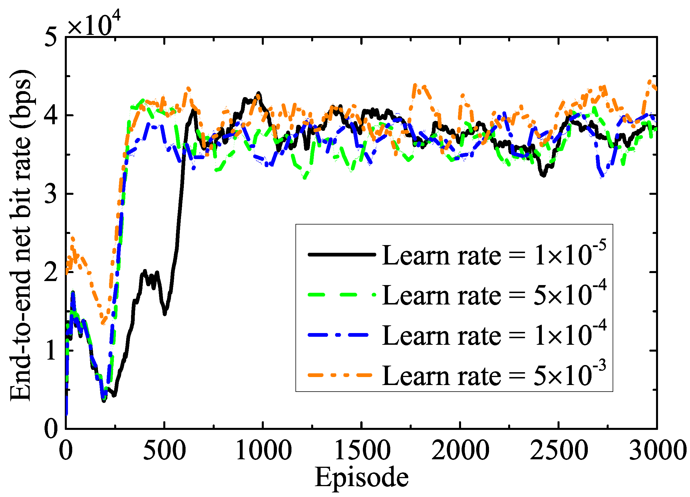
Figure 2 demonstrates the converging behavior of the training performance at dB noise power for various learning rates under the QPSK modulation scheme. According to this figure, the end-to-end net bit rate increases with each episode and eventually converges. If we choose a low learning rate, the training process runs slowly, because the low learning rate updates the NNs’ weights on a small scale. However, if we set a high learning rate, the loss function of the NNs encounters undesirable divergence. Consequently, the NNs experience high oscillation during training, but the objective value converges quickly. This figure shows that fluctuations and convergence rates over the training episode increase when the learning rate varies from to . Hence, considering the model’s stability, we set the learning rate to for the subsequent simulations.
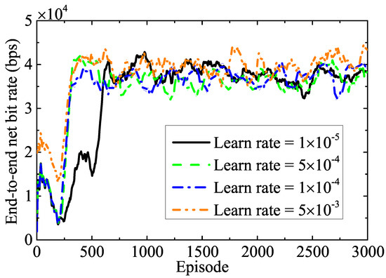
Figure 2.
Impact of different learning rate values on the convergence.
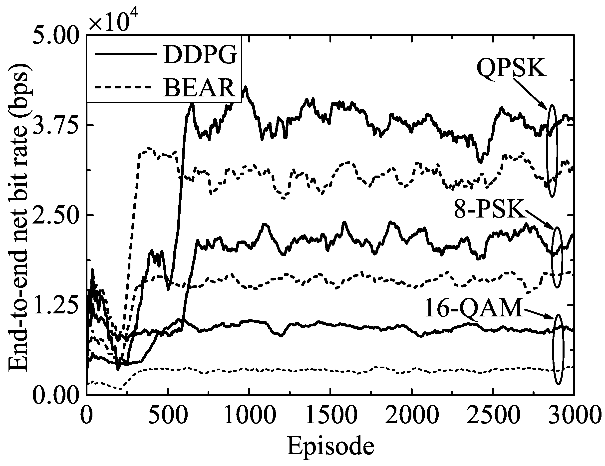
Figure 3 presents the variation of the end-to-end net bit rate over the training episodes to analyze the performance of the proposed and benchmark algorithms corresponding to different modulation schemes, while the noise power was set to dB. This figure shows that the converged objective value increased with the lower modulation schemes because this required less power and fewer signal points to transmit the same amount of data, which allowed a more efficient use of the available frequency spectrum. Therefore, QPSK achieved a higher end-to-end net bit rate than 8-PSK and 16-QAM. Furthermore, as the benchmark BEAR algorithm entailed more computational complexity, due to the off-policy samples from the replay buffer, the achievable performance metric corresponding to the BEAR algorithm was lower than the proposed DDPG algorithm. Hence, according to this figure, the DDPG algorithm outperformed the BEAR algorithm by , , and in the cases of the QPSK, 8-PSK, and 16-QAM modulation schemes, respectively.

Figure 3.
Performance comparison of the proposed DDPG and the benchmark BEAR algorithms for various modulation schemes.
5.2. Performance Evaluation
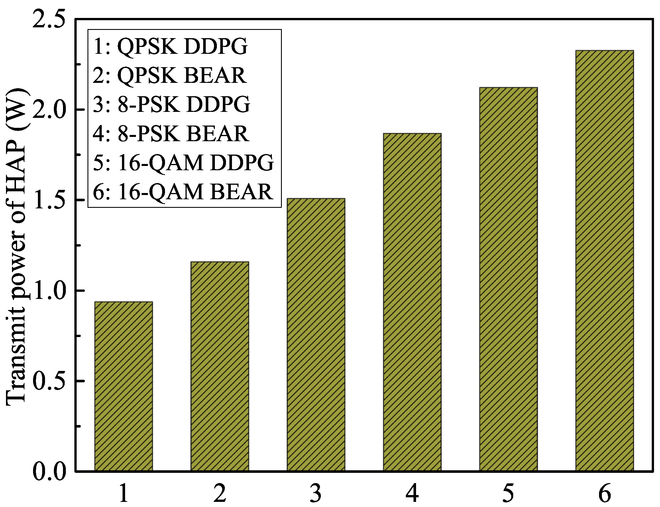
We plot the transmit power variation of the HAP in Figure 4, corresponding to the proposed and benchmark algorithms for different modulation schemes. It can be observed that the average transmit power of the HAP increased with the higher modulation schemes because they required higher peak-to-average power ratios and higher transmit power levels to generate complex signal constellations. On the other hand, the conventional BEAR algorithm updated the parameters of the policy evaluation NN using a distributional shift correction method to reduce the overestimation of the Q-value. This limited the ability of the algorithm to explore the search space and find optimal policies in complex environments. From Figure 4, it is clear that the proposed methodology reduced the average transmit power of the HAP by , , and as compared to the BEAR algorithm in the cases of the QPSK, 8-PSK, and 16-QAM modulation schemes, respectively, over the operational period.
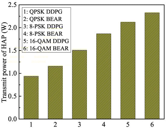
Figure 4.
Transmit power variation of the HAP over the operational period.
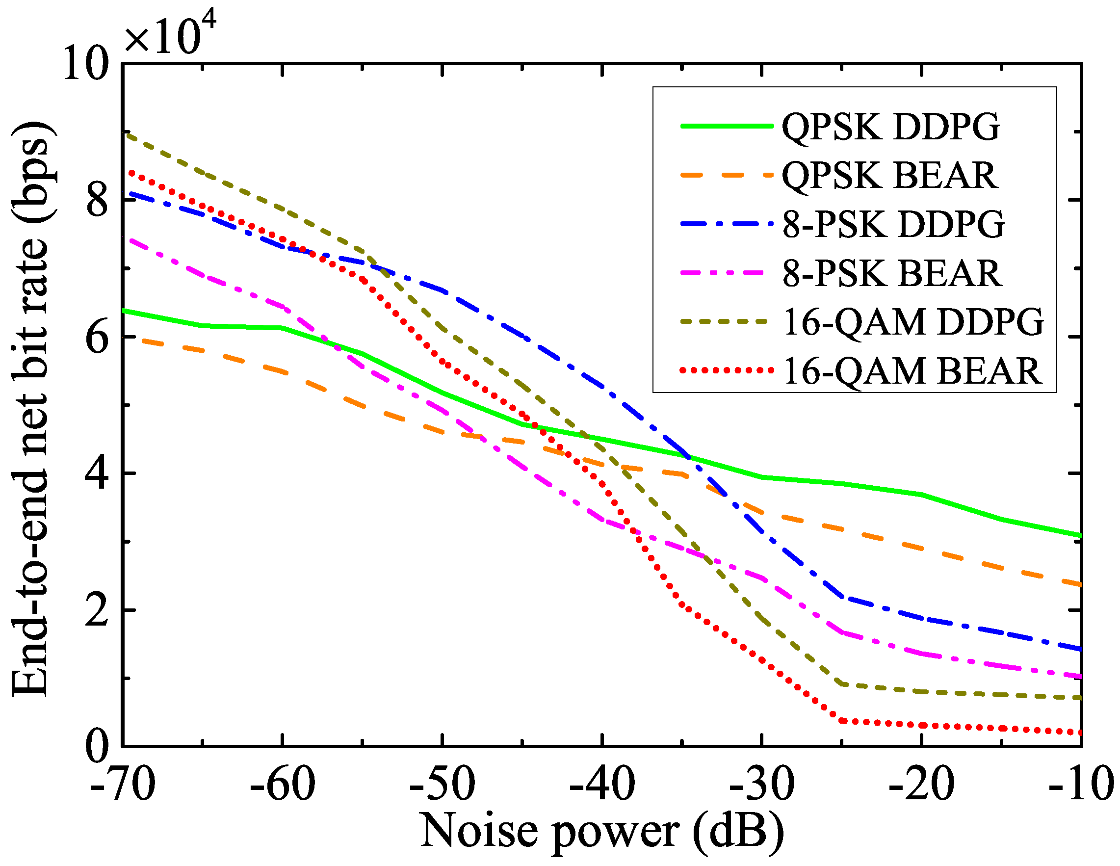
Figure 5 illustrates the end-to-end net bit rate for the different modulation schemes under various noise power levels at the receiver. This figure shows that the 16-QAM modulation scheme performed better than 8-PSK and QPSK at a lower noise power, whereas QPSK outperformed 8-PSK and 16-QAM at a higher noise power. This is because the higher modulation schemes encode more bits per symbol, which allows higher data rates to be transmitted over a given channel bandwidth. However, since they typically use more complex signal constellations with smaller distances between signal points, they are highly susceptible to the distortion caused by noise or channel impairments. On the other hand, the lower modulation techniques are more straightforward to implement than the higher modulation techniques. This makes them more suitable for low-power at low-complexity systems, making them more bandwidth-efficient at a higher noise power. From Figure 3 and Figure 4, we can justify that the benchmark BEAR algorithm faced several challenges in finding the optimal policy. Hence, the proposed DDPG algorithm improves the performance metric by , , and as compared to the BEAR algorithm in the cases of the QPSK, 8-PSK, and 16-QAM modulation schemes, respectively.
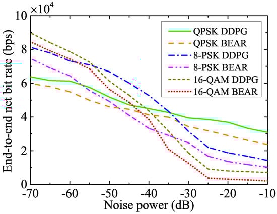
Figure 5.
Net bit rate using the different modulation schemes for a wide range of noise powers.
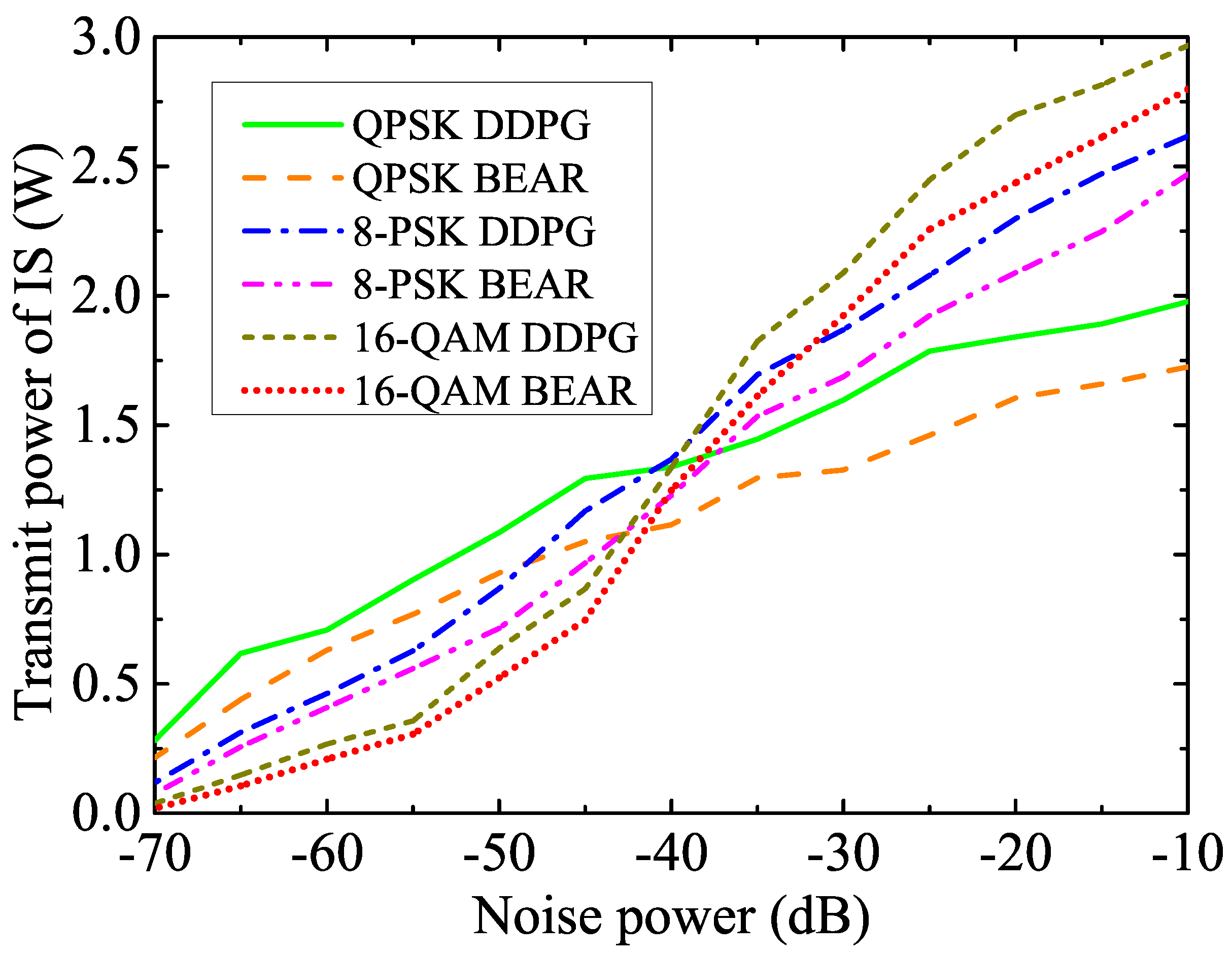
The variation of the allotted IS’s transmit power with respect to the noise power under different modulation techniques is shown in Figure 6. It can be observed that the transmit power of the IS increased with the noise power because the IS utilized more transmit power to achieve a minimum SNR and BER value for a higher noise power, which also maintained an adequate quality of service (QoS). Since we mentioned earlier that higher modulation techniques are more susceptible to distortion caused by channel noise impairments, 16-QAM requires more transmit power at higher noise power levels compared to the 8-PSK and QPSK modulation techniques. Moreover, as the benchmark algorithm is inefficient, the proposed technique reduced the transmit power of IS by , , and compared to the BEAR algorithm in the cases of the QPSK, 8-PSK, and 16-QAM modulation schemes, respectively.
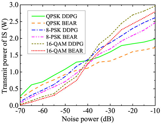
Figure 6.
Transmit power variation of IS with different modulation schemes for various noise powers.
6. Conclusions
Facing the great challenges of reliable WPCN, this article introduced a JIER protocol that allocates resources efficiently, for effective energy management in EH wireless networks. Specifically, the formulated joint optimization of HAP and IS transmit power, the fraction of harvested energy transmitted by relays, and relay selection indicators maximized the end-to-end net bit rate of the system under energy borrowing and return scheduling constraints. The formulated problem was highly non-convex, nontrivial, and difficult to solve directly. Hence, we leveraged the DRL framework, which decomposed the original problem into multiple sub-problems based on MDP, and then proposed the DDPG algorithm to find the optimal policy. The simulation results validated the proposed scheme and enhanced the end-to-end net bit rate of the system by , , and compared with the BEAR algorithm for the QPSK, 8-PSK, and 16-QAM modulation schemes, respectively. In the future, we will extend this work to an energy borrowing and returning strategy in multi-user and multi-antenna relay-assisted EH systems using multi-agent DRL, where the objective will be the minimization of the age of information, to ensure a tolerable latency.
Author Contributions
Conceptualization, A.M., M.S.A., D.M. and G.P.; formal analysis, A.M. and M.S.A.; funding acquisition, D.M.; investigation, A.M. and M.S.A.; methodology, A.M. and M.S.A.; project administration, G.P. and D.M.; resources, A.M., M.S.A., D.M. and G.P.; software, A.M. and M.S.A.; supervision, D.M. and G.P.; validation, A.M. and M.S.A.; writing— original draft, A.M. and M.S.A.; writing—review and editing, A.M., M.S.A., D.M. and G.P. All authors have read and agreed to the published version of the manuscript.
Funding
D. Mishra’s participation was partially funded by the Australian Research Council Discovery Early Career Award (DECRA)-DE230101391.
Data Availability Statement
The data of this paper is available through e-mail via authors.
Conflicts of Interest
The authors declare no conflict of interest.
References
- Bi, S.; Zeng, Y.; Zhang, R. Wireless powered communication networks: An overview. IEEE Wirel. Commun. 2016, 23, 10–18. [Google Scholar] [CrossRef]
- Lin, H.C.; Chen, W.Y. An approximation algorithm for the maximum-lifetime data aggregation tree problem in wireless sensor networks. IEEE Trans. Wirel. Commun. 2017, 16, 3787–3798. [Google Scholar] [CrossRef]
- Lu, X.; Wang, P.; Niyato, D.; Kim, D.I.; Han, Z. Wireless charging technologies: Fundamentals, standards, and network applications. IEEE Commun. Surv. Tutor. 2016, 18, 1413–1452. [Google Scholar] [CrossRef]
- Lee, K.; Choi, H.-H.; Lee, W.; Leung, V.C.M. Wireless-Powered Interference Networks: Applications, Approaches, and Challenges. Veh. Technol. Mag. 2015; early access. [Google Scholar] [CrossRef]
- Hsieh, P.H.; Chou, C.H.; Chiang, T. An RF energy harvester with 44.1% PCE at input available power of −12 dbm. IEEE Trans. Circuits Syst. 2015, 62, 1528–1537. [Google Scholar] [CrossRef]
- Tutuncuoglu, K.; Yener, A. Energy harvesting networks with energy cooperation: Procrastinating policies. IEEE Trans. Commun. 2015, 63, 4525–4538. [Google Scholar] [CrossRef]
- Mishra, D.; De, S. Optimal relay placement in two-hop RF energy transfer. IEEE Trans. Commun. 2015, 63, 1635–1647. [Google Scholar] [CrossRef]
- Ju, H.; Zhang, R. User cooperation in wireless powered communication networks. In Proceedings of the IEEE Global Communications Conference, Austin, TX, USA, 8–12 December 2014; pp. 1430–1435. [Google Scholar] [CrossRef]
- Chen, H.; Li, Y.; Rebelatto, J.L.; Uchoa-Filho, B.F.; Vucetic, B. Harvest-then-cooperate: Wireless-powered cooperative communications. IEEE Trans. Signal Process. 2015, 63, 1700–1711. [Google Scholar] [CrossRef]
- Gu, Y.; Chen, H.; Li, Y.; Vucetic, B. An adaptive transmission protocol for wireless-powered cooperative communications. In Proceedings of the IEEE International Conference on Communications (ICC), London, UK, 8–12 June 2015; pp. 4223–4228. [Google Scholar] [CrossRef]
- Sarma, S.; Ishibashi, K. Time-to-recharge analysis for energy-relay-assisted energy harvesting. IEEE Access 2019, 7, 139924–139937. [Google Scholar] [CrossRef]
- Na, Z.; Lv, J.; Zhang, M.; Peng, B.; Xiong, M.; Guan, M. GFDM based wireless powered communication for cooperative relay system. IEEE Access 2019, 7, 50971–50979. [Google Scholar] [CrossRef]
- Wei, Z.; Sun, S.; Zhu, X.; Kim, D.I.; Ng, D.W.K. Resource allocation for wireless-powered full-duplex relaying systems with nonlinear energy harvesting efficiency. IEEE Trans. Veh. Technol. 2019, 68, 12079–12093. [Google Scholar] [CrossRef]
- Gurakan, B.; Ozel, O.; Ulukus, S. Optimal energy and data routing in networks with energy cooperation. IEEE Trans. Wirel. Commun. 2016, 15, 857–870. [Google Scholar] [CrossRef]
- Huang, X.; Ansari, N. Energy sharing within EH-enabled wireless communication networks. IEEE Wirel. Commun. 2015, 22, 144–149. [Google Scholar] [CrossRef]
- Hu, C.; Gong, J.; Wang, X.; Zhou, S.; Niu, Z. Optimal green energy utilization in MIMO systems with hybrid energy supplies. IEEE Trans. Veh. Technol. 2015, 64, 3675–3688. [Google Scholar] [CrossRef]
- Sun, Z.; Dan, L.; Xiao, Y.; Wen, P.; Yang, P.; Li, S. Energy borrowing: An efficient way to bridge energy harvesting and power grid in wireless communications. In Proceedings of the IEEE 83rd Vehicular Technology Conference, Nanjing, China, 15–18 May 2016; pp. 1–5. [Google Scholar] [CrossRef]
- Sun, Z.; Dan, L.; Xiao, Y.; Yang, P.; Li, S. Energy borrowing for energy harvesting wireless communications. IEEE Commun. Lett. 2016, 20, 2546–2549. [Google Scholar] [CrossRef]
- Cui, J.; Ding, Z.; Deng, Y.; Nallanathan, A.; Hanzo, L. Adaptive UAV-trajectory optimization under quality of service constraints: A model-free solution. IEEE Access 2020, 8, 112253–112265. [Google Scholar] [CrossRef]
- Challita, U.; Saad, W.; Bettstetter, C. Interference management for cellular-connected UAVs: A deep reinforcement learning approach. IEEE Trans. Wirel. Commun. 2019, 18, 2125–2140. [Google Scholar] [CrossRef]
- Liu, Z.P.; Zhou, M.G.; Liu, W.B.; Li, C.L.; Gu, J.; Yin, H.L.; Chen, Z.B. Automated machine learning for secure key rate in discrete-modulated continuous-variable quantum key distribution. Opt. Express 2022, 30, 15024–15036. [Google Scholar] [CrossRef]
- Qiu, C.; Hu, Y.; Chen, Y.; Zeng, B. Deep deterministic policy gradient (DDPG)-based energy harvesting wireless communications. IEEE Internet Things J. 2019, 6, 8577–8588. [Google Scholar] [CrossRef]
- Zhao, B.; Zhao, X. Deep reinforcement learning resource allocation in wireless sensor networks with energy harvesting and relay. IEEE Internet Things J. 2022, 9, 2330–2345. [Google Scholar] [CrossRef]
- Sachan, A.; Mishra, D.; Prasad, G. BEAR: Reinforcement learning for throughput aware borrowing in energy harvesting systems. In Proceedings of the IEEE Global Communications Conference (GLOBECOM), Madrid, Spain, 7–11 December 2021; pp. 1–6. [Google Scholar] [CrossRef]
- Su, Y.; Lu, X.; Zhao, Y.; Huang, L.; Du, X. Cooperative communications with relay selection based on deep reinforcement learning in wireless sensor networks. IEEE Sens. J. 2019, 19, 9561–9569. [Google Scholar] [CrossRef]
- Wei, Y.; Yu, F.R.; Song, M.; Han, Z. User scheduling and resource allocation in hetnets with hybrid energy supply: An actor-critic reinforcement learning approach. IEEE Trans. Wirel. Commun. 2018, 17, 680–692. [Google Scholar] [CrossRef]
- Masadeh, A.; Wang, Z.; Kamal, A.E. An actor-critic reinforcement learning approach for energy harvesting communications systems. In Proceedings of the International Conference on Computer Communication and Networks, Valencia, Spain, 29 July–1 August 2019; pp. 1–6. [Google Scholar] [CrossRef]
- Reddy, G.K.; Mishra, D.; Devi, L.N. Scheduling protocol for throughput maximization in borrowing-aided energy harvesting system. IEEE Netw. Lett. 2020, 2, 171–174. [Google Scholar] [CrossRef]
- Kumari, M.; Prasad, G.; Mishra, D. Si2ER protocol for optimization of RF powered communication using deep learning. In Proceedings of the IEEE Wireless Communications and Networking Conference (WCNC), Austin, TX, USA, 10–13 April 2022; pp. 10–13. [Google Scholar] [CrossRef]
Disclaimer/Publisher’s Note: The statements, opinions and data contained in all publications are solely those of the individual author(s) and contributor(s) and not of MDPI and/or the editor(s). MDPI and/or the editor(s) disclaim responsibility for any injury to people or property resulting from any ideas, methods, instructions or products referred to in the content. |
© 2023 by the authors. Licensee MDPI, Basel, Switzerland. This article is an open access article distributed under the terms and conditions of the Creative Commons Attribution (CC BY) license (https://creativecommons.org/licenses/by/4.0/).