2. Literature Review
Poland’s energy policy until 2040 assumes a 75% increase in solar power capacity by 2040 [
3]. Solar energy is a type of renewable energy that has been subjected to continuous dynamic development since the 1980s. Therefore, many examples of PV power forecasting can be found in the literature. Taking into account the time horizon of forecasts, they can be divided into very short-term, limited to second and hour forecasts [
4], short-term, characteristic for daily forecasts [
5], and medium-term, covering weeks or months. Long-term forecasts, in turn, cover years [
6]. Additionally, the PV power forecasting methods used so far can be divided into direct forecasts where historical PV power is used. In turn, the indirect method involves forecasting PV power generation based on weather data and historical data on solar irradiation [
7].
To predict PV power, methods such as artificial neural networks (ANN) were used [
8]. The ANN method has also been subjected to numerous modifications to optimize it. Short-term neural networks (STM), long short-term memory (LSTM) [
9], support vector machine (SVM) [
10], or fuzzy logic (FL) [
11] have also been applied.
Grey prediction model was used for long-term forecasts, the advantage of which is that it requires a small amount of historical data [
12,
13]. Due to the nature of the solar energy consumption time series, a modified Grey model was also applied, which had a positive effect on the accuracy of the prediction [
14]. Markov chains [
15] as well as ARIMA [
16], SARIMA [
17], Vector Autoregression VAR [
18], and Support Vector Regression SVR [
19] models were used for PV power prediction.
In the literature, examples of the use of linear regression to forecast all aspects related to the production of PV power can also be found [
5], including multiple regression [
20]. Yang and Meng used 12 independent weather variables from the European Centre for Medium-Range Weather Forecasts [
21].
In turn, the authors of this publication used the indirect method and built their own set of explanatory data, taking into account economic, ecological, and technological factors, as well as energy and raw materials factors. The forecast proposed by the authors constitutes a long-term forecast until 2025. The prediction and model verification methods used are described in the Methods section.
3. Advantages and Disadvantages of the Model Used to Forecast PV Power
The main advantage of ANN models is the self-learning ability of the neural network. Thanks to this, it can improve the results of the forecasts it generates. Neural networks find solutions that are often not obvious to humans. Additionally, neural networks are able to adapt to changing explanatory variables. The main disadvantage of ANNs is that they work similar to black boxes, i.e., it is not entirely clear why they gave a specific result. An additional problem arises in the case of unique and complex tasks that will require a lot of time and resources to complete. Additionally, learning the neural network requires the provision of a large amount of data, which, for example, in the case analyzed in the article is not entirely possible due to the limited length of the PV power generation time series [
22,
23]. Despite numerous advantages, it was noticed that there are significant differences between the real data and the results obtained thanks to ANN. The MAPE error in this case ranges from 5–8% [
24]. SVM methods usually provide more accurate results than independent methods, but their disadvantage is the need to perform a large number of calculations related to repeated network training. With large amounts of data, model estimation may take a long time and estimating the correct model requires some knowledge. Because a support vector classifier works by placing data points above and below the classification hyperplane, there is no probabilistic explanation for classification [
25,
26]. The MAPE errors of the SVM models ranged from 5% for annual forecasts to 16% for daily forecasts [
27]. Because FL models belong to the group of expert systems, they lead to imprecise data. Qualitative analysis based on fuzzy data enables assessments and summaries to be made in natural language, in a form understandable to an average user. They are suitable for solving problems where high accuracy is not needed and there is no systematic method for designing these systems. The MAPE based on the fuzzy logic algorithm ranges from 13.87% to 20.22% for solar radiation forecasting [
28]. The main advantages of grey models include the ease of calculations and short forecast preparation time. The main disadvantages include the failure to meet the conditions set for the residuals of the econometric model [
29]. The MAPE error for the Grey model found in the literature ranged from 3–7% [
30,
31]. Markov models can be used when there are multiple causes of the phenomenon under study, as well as in the case of qualitative variables. Using Markov chains, short-, medium-, and long-term forecasts can be created [
32]. The best forecasting results for the PV power were obtained using a combination of the Markov model and the generalized fuzzy model. In this case, the MAPE error was approximately 7% [
33]. In turn, ARMAX class models are popular due to the automation of the time series decomposition process. At the same time, they provide great flexibility in selecting the right model. This allows to take into account variables that are important from the point of view of the analyzed process. Automation of the estimation process allows quick determination and comparison of many potential models [
34]. ARMA was used for short- and medium-term forecasts at the microgrid level. It has been noticed that it works well for very short-term forecasting [
35]. The MAPE error for the models made with this method was approximately 16% [
36].
Inspection of statistical criteria showed that the lowest RMSE values were recorded when the MLR model included extraterrestrial radiation, the difference between the maximum and minimum daily temperature, and relative humidity as input variables [
37]. One of the main advantages of multiple regression is that it can capture the complex and multifaceted nature of real-world phenomena. This gives a more accurate and detailed picture of the relationship between each specific factor and the outcome. The greatest advantage of linear regression models is linearity because it simplifies the estimation procedure and linear equations are easy to understand at the modular level. Another advantage is the ability to identify outliers, i.e., anomalies, and the ability to determine the relative impact of one or more predictor variables on the criterion value. The disadvantages of using a multiple regression model usually lie in the data used. First, a problem may arise when incomplete data are used. Attention should also be paid to the assumptions and conditions of multiple regression, such as linearity, normality, and homoscedasticity. These should be verified using statistic tests. If these assumptions are violated, the results may be inaccurate or misleading.
The authors decided to choose multiple regression for their research, which is suitable for long-term forecasts. The simple and transparent structure of the model makes the interpretation of the obtained results much easier than, for example, in the case of neural networks. The MLR model allowed operating on relatively short time series, which would be impossible in the case of many of the other methods mentioned. Additionally, the calculation speed in this case is much faster than in the case of models that undergo a learning process. The MLR model also meets the assumptions and requirements of the residuals of the econometric models. Appropriate statistical tests allow to verify the assumptions of normality, lack of autocorrelation, and homoscedasticity of residuals. The authors also assumed that the MLR model would be characterized by a high level of accuracy of the obtained forecasts.
Table 1 presents a summary of the features of the most common models used to forecast PV power generation in the literature and features of the model due to which the model could not be used in the case of the PV power generation in Poland time series.
To summarize the above considerations, the aim of the research was to find a simple model, easy to use, and with a transparent structure, which would allow the identification of factors influencing the size of PV power generation in Poland in the long term (in years).
Before looking for a nonlinear model, it is best to first use a linear model such as AMRAX or MLR. The most commonly used MLR examines the relationship between power output and climatic factors [
38]. In turn, the authors took into account not climatic factors, but ecological, economic, raw material, and energy factors. At the same time, it was important in the presented research to determine a model that would be characterized by high accuracy of the forecasts created. Based on their forecasting experience, the authors initially selected two models, i.e., the ARMAX and MLR models. Both of them meet the conditions set. The authors assumed that by applying all the requirements for time series and model residuals, they would be able to find a model with MAPE error values at least at the level obtained for more complicated tools, such as ANN or SVM.
4. Methods
Multiple linear regression MLR is a statistical method that uses many explanatory variables to predict the value of the explained variable. It enables the study of the linear relationship between the dependent variable and the independent variables that influence it.
Multiple regression allows to describe the relationship between one explained variable and many independent variables. Due to this, it is possible to examine which of them best describe the explained variable [
39].
The multiple regression model can be described by the following equation:
where:
z—dependent variable,
—random variable,
—regression coefficient,
—explanatory variables.
The regression coefficients of the model β characterize the contribution of each explanatory variable in the forecasting process of the explained variable. The sign of the correlation coefficient determines the nature of the relationship between the individual variables. A positive sign means that the variable is a stimulant, i.e., an increase in the independent variable has a positive effect on the value of the explained variable. A negative sign, in turn, means that an increase in the explanatory variable has a negative impact on the explained variable (destimulant). A correlation coefficient of 0 would mean that there is no relationship between the variables.
The primary methodological limitation underlying MLR is that it can only be used to establish the existence of an association, but cannot determine the causes underlying that association. Another limitation is the number of explanatory variables that can be introduced into the model. It is recommended to include at least 10–20 times as many observations as the number of variables in the analysis. This may lead to the omission of important variables. MLR also only allows for the analysis of linear relationships between variables, which is also a serious limitation.
Forecasting based on a nonstationary time series may produce erroneous results. Since the time series used by the authors to build the MLR model may be characterized by a trend, the results obtained may be questionable and lead to the appearance of the phenomenon of spurious regression. Therefore, before searching for the optimal MLR model, it is necessary to verify the hypothesis that the time series is stationary. For this purpose, for example, the Dickey–Fuller test can be used.
The statistics of the Dickey–Fuller test (DF) for the existence of a unit root are represented by the formula:
The DF test allows to verify whether there is a unit root in a time series. The test requires verification of the following hypotheses:
H0: there is a unit root in the time series,
H1: the time series is stationary, .
If the ADF test confirms the existence of nonstationarity in the time series, it can be eliminated by differentiating the series or introducing a time variable into the model [
40].
Building an econometric model burdened with autocorrelation may also lead to conclusions based on an incorrect model. To verify the occurrence of autocorrelation, the Durbin–Watson test was used [
41]. This is one of the most frequently used tests, which is based on the assumption that if random disturbances contain autocorrelation, the residuals of the model will also be correlated. The test requires the null hypothesis H0—the residuals of the model are not correlated with each other—and the alternative hypothesis H1—there occurs autocorrelation in the residuals of the model.
where:
—Durbin–Watson test statistic,
—the residuals of the model,
T—length of the sequence of residues.
One of the assumptions of the regression model is also the normality of the residual term. Therefore, the normality of the distribution of model residuals was confirmed using the Doornik–Hansen test statistics DH [
42]:
where:
—transformed sample skewness,
—Wilson–Hilferty transformation.
The heteroscedasticity of a time series means that at least one random variable in the sequence differs from the others in variance or its variance is infinite [
43]. The occurrence of heteroscedasticity may indicate an incorrect form of the model or omission of important variables.
The Breusch–Pagan test for heteroskedasticity is used when it is caused by more than one variable. The test requires two hypotheses: H0—there is homoscedasticity in the model—and hypothesis H1—there is heteroscedasticity in the model. The formula for the Breusch–Pagan test statistics is as follows:
where:
—Breusch–Pagan statistic,
ESS—Explained Sum of Squares in auxiliary regression.
In addition, the models created were analyzed in terms of information criteria [
44]. When comparing several similar models, the one with the lowest Akaike (AIC), Schwarz (BIC), and Hannan–Quinn (HQ) criteria values should be chosen:
where:
n—number of observations,
—model credibility function corrected by the penalty function—the function of the number of K parameters of the model.
The model was also selected based on the value of ex post errors. Several of them were taken into account, namely:
Mean Absolute Error (
MAE) [
45]:
Root Mean Square Error (
RMSE) [
46,
47]:
Mean Absolute Percentage Error (
MAPE) [
48,
49]:
where:
—value of the explained variable in period t,
—forecast error.
Theil’s inequality coefficient (
U) [
50]:
where:
—empirical value,
—forecast of the explained variable in period t.
5. Results and Discussion
ARMAX and MLR models were initially built. However, the AMRAX models were ultimately rejected because, depending on the combination of explanatory variables and the adopted model parameters, the MAPE error ranged from 3–30%.
The research began by collecting statistical data on factors that could influence the volume of PV power generation in Poland. The analysis was aimed at identifying not the weather factors and technical parameters of the solar panels, which, as discussed in the Introduction, are the most frequently the subject of interest, but ecological, economic, raw material, and energy factors. The factors that were finally taken into account and the source of their acquisition are presented in
Table 2.
The value of the explained variable was approximated by a mathematical model. This was possible because the explanatory variables in the past were characterized by regular changes that could be described using time functions. The direction of the trend and changes in the analyzed phenomena were assumed to be constant. It was also assumed that random fluctuations did not significantly affect the nature of the analyzed phenomenon. However, these assumptions were supplemented by using scenarios in which it was assumed that possible changes in the explanatory variables may ultimately affect the explained variable.
Forecasting using the MLR model was carried out in the following steps:
Specification—visual analysis of time series, determining the nature of regularities occurring in the time series of explanatory variables and the explained variable.
Estimation of parameters of the MLR function, when selecting explanatory variables for the MLR model, general guidelines for econometric models were used.
For the coefficient of variation, those variables whose coefficient of variation is greater than 0.1 were selected. For the variables finally entered into the model, the coefficient of variation was on average 0.8.
The explanatory variables should be strongly correlated with the explained variable—in the case of most variables, the correlation coefficient was from 0.99–0.7. Only in the case of primary energy consumption was this condition not met. However, the parameter turned out to be statistically significant. It is also known that these assumptions can be 100% met only for experimental data. Due to the importance of this variable in terms of the research being conducted, it was retained in the model.
Verification—examination of compliance of designated models with empirical data, verification of information criteria, ex post errors, examination of model residuals in terms of normality of distribution, autocorrelation, and homoscedasticity.
Prediction—a proven and accepted model was used to build a forecast in the selected horizon.
Since electricity generated using solar panels has been produced in Poland only since 2011, and the authors wanted to make a long-term forecast that required annual data, the analyzed time series is relatively short. Therefore, it was impossible to introduce more than eight explanatory variables into the models due to the insufficient number of freedom degrees. Therefore, the authors selected the categories variables for each of the analyzed that were considered the most representative. For economic factors, these were the LCOE (levelized cost of electricity) and real GDP (gross domestic product) per capita for ecological factors, the amount of CO2 emission for energy factors, installed capacity, gross available energy, final energy consumption, and primary energy consumption. The raw materials category considered the share of natural raw materials necessary to produce MW installed in Poland during the year in the annual production/import of a given raw material in Poland. Raw materials taken into account are critical raw materials, such as copper (Cu), gallium (Ga), germanium (Ge), and silicon (Si).
To determine the demand for critical raw materials in accordance with the expected level of installed power, the WEKR 2.0 computer program written by research authors was used. The data necessary to perform the appropriate calculations were taken from Ref. [
55].
Figure 1 presents the algorithm according to which the program calculates the value of explanatory variables from the category of raw materials. First, the program determines how many MW will be produced in Poland annually by 2025. The next step determines the number of kilograms of each critical raw material needed to generate the installed capacity planned for a given year.
When selecting the forecast model, the authors took into account the ARMAX and MLR models. MAPE error was chosen as the model comparison indicator so that the accuracy of the MLR model could be compared with models found in the literature and presented in this publication. It was noted that the constructed ARMAX models were characterized by a minimum MAPE error of 3%, while the MAPE of the MLR model was 0.87%. This is an excellent result also compared to models such as ANN, SVM, or FL, the development of which is much more complicated and requires more time and resources. Therefore, the MLR model was finally selected for analysis. Due to this, it was possible to take into account all explanatory variables when building a model of annual PV power production in Poland until 2025. The variable explained in the volume of built model was the PV power production. Due to the limited possibility of introducing all explanatory variables into the model at the same time, the forward stepwise method was used, which involves introducing individual factors into the model one by one, ending when adding another factor does not significantly improve the prediction. In the model, a combination of explanatory variables was retained, where all these variables were statistically significant. Since the ADF test showed that the analyzed time series is nonstationary with probability
p = 0.99, an additional time variable t was introduced into the model; otherwise, the model being built could give erroneous results.
Table 3 shows the explanatory variables that were finally selected to build the model. A statistically significant impact on the volume of PV power generation was characteristic for CO
2 emissions, LCOE, copper consumption, primary energy consumption, the number of reported patents related to PV technology, GDP, and installed capacity.
The parameter value column contains the value of the regression coefficient for individual explanatory variables. The probability column contains the value of statistical significance p. Statistical significance was verified with the Student’s t-test. Two hypotheses were presented:
H0—the variable is not statistically significant,
H1—the variable is statistically significant.
If p is less than the significance level α, it is necessary to reject hypothesis H0 in favor of hypothesis H1. If it is greater than the significance level, the H0 hypothesis should be maintained. Only variables where p was lower than α = 0.01 (***) and α = 0.05 (**) were entered into the model.
The last column of
Table 2 contains information on the nature of the explanatory variables. LCOE, CO
2 emissions, and copper consumption are destimulants. This means that an increase in these explanatory variables has a negative impact on the volume of PV power generation. In the case of the LCOE, it is obvious that a decrease in the cost of generating PV power stimulates further investment. The decrease in the volume of photovoltaic power production will, in turn, require filling the gap with the energy produced based on fossil fuels, which will translate into an increase in CO
2 emissions. The intense (exponential) increase in copper demand that has been taking place since 2018 may lead to rapid consumption of this raw material, which may be a factor limiting the further development of PV farms in the future. The remaining explanatory variables are stimulants, which means that their increase stimulates the increase in PV power generation.
The adopted model was verified in terms of the information criteria values, as well as ex post errors, which are presented in
Table 4. The MAPE error is used to compare potential models. The model selected for further analysis is characterized by a very low MAPE error value below 1%. This means that the model can be considered highly reliable and accurate. The coefficient of determination (R2) is also 0.99, which means that 99% of the empirical data entered into the model were described by this model.
The model was used to determine the forecast and ultimately the residuals of the model. The residuals were analyzed for heteroskedasticity, normal distribution, and autocorrelation.
The Breusch–Pagan test for heteroskedasticity showed that there is no heteroskedasticity phenomenon in the model. The obtained
p-value was greater than the assumed significance level alpha = 0.01.
Because the model is characterized by the homoscedasticity of the random component variance, it can be used for correct statistical inference.
The residuals of the model were also verified for normal distribution. For this purpose, the Doornik–Hansen test was used. The test confirmed the correctness of the null hypothesis, which means that the empirical distribution function has a normal distribution with a probability value of
p = 0.38654 > α = 0.05.
The residuals of a properly constructed econometric model should not show autocorrelation, that is, the dependence of current values of the random component on past values. To check whether the residuals of the adopted model constitute white noise, the Durbin–Watson test was used. It confirmed the validity of the H0 hypothesis on the lack of correlation of residuals. The probability value p in this case was p = 0.365725 > α = 0.05.
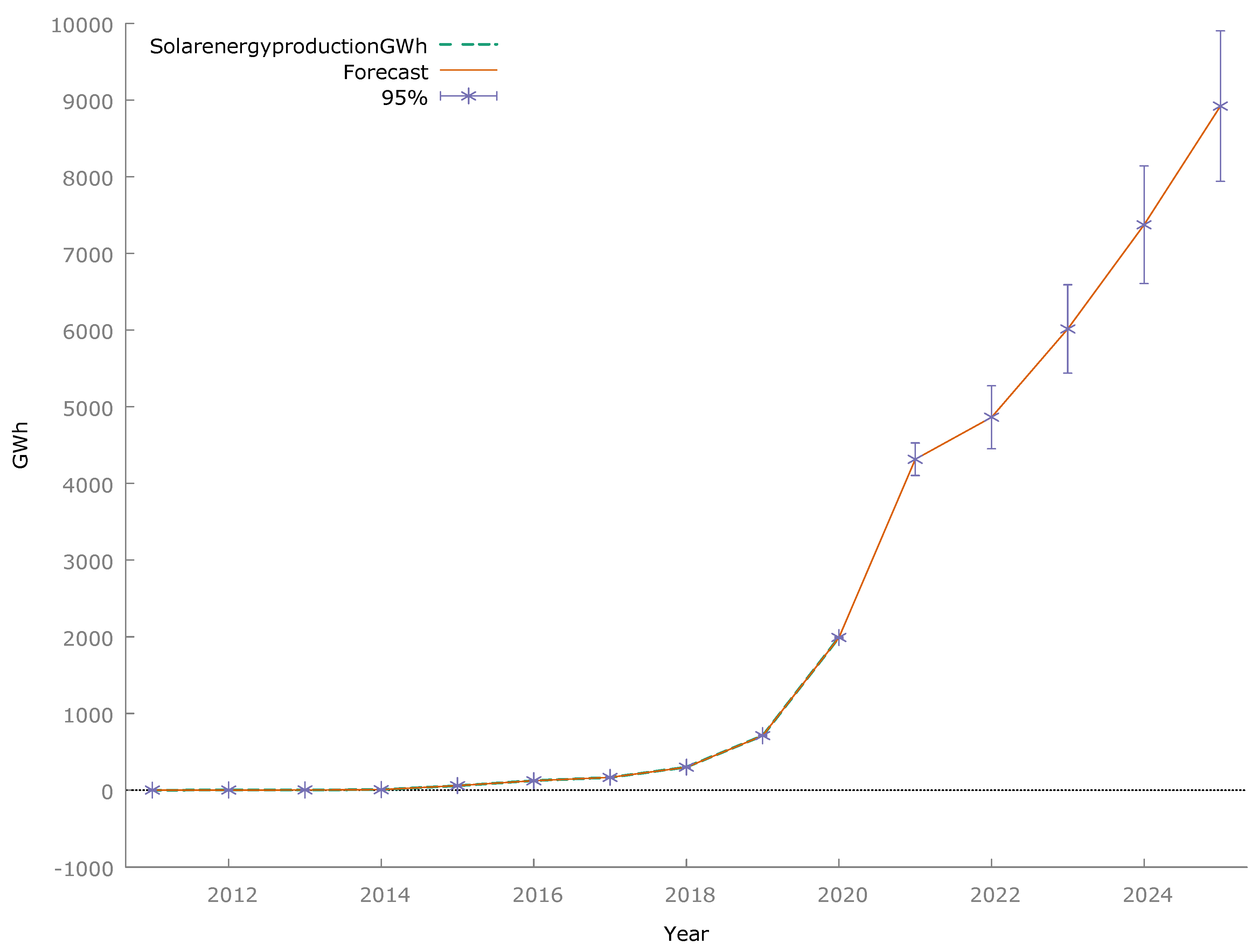
Because the model was successfully validated and met all the conditions for linear regression models, it was used to build a forecast of the PV power production volume until 2025. The empirical data, the forecast, and the confidence interval for the forecast are presented in
Figure 2.
It should be noted that the visual analysis of time series of empirical and theoretical data also indicates the high accuracy of the multiple regression model. If the explanatory variables introduced into the model continue to be subject to the same trends shaping them, a dynamic increase in PV power generation should be expected until 2025. The built model indicates that the Poland Energy Policy until 2040 (PEP2040) goal of expanding the installed capacity to 16 GW by 2040 could be achieved as early as 2025. To determine this value, a conversion factor was used, obtained by determining the average value of photovoltaic power generation to the installed power in 2011–2020. The volume of PV power production in 2025 would be, according to the forecast, 8.921 GWh, which is more than four times the last known observation from 2020.
The year 2022 is the period of the most intensive development of photovoltaic technology in Poland. The reason for the unprecedented interest in this solution was primarily the war in Ukraine, rising electricity prices, and concerns about the lack of access to energy resources. Moreover, the state’s encouragement in connection with the implementation of PEP2040 and the National Reconstruction Plan in the form of tax reliefs and co-financing programs translated into an increase in the number of photovoltaic installations in Poland. In 2022, the number of prosumer installations increased by 40% compared to the previous year. The increase in interest in photovoltaic installations was also influenced by the decrease in energy generation, the need to reduce greenhouse gas emissions, the increasing demand for electricity with the simultaneous threat of lack of access to energy (energy raw materials), and the economic development of the country. According to the Energy Regulatory Office [
56], 74% of the total installed capacity were private installations. However, April 2022 brought a change to the settlement system for prosumers based on net-billing. As a result of this change, interest in photovoltaic installations in Poland has decreased. In the first quarter of 2023, it decreased by approximately 30% [
57]. Therefore, due to the upcoming changes, investors interested in PV installations expressed their willingness to connect to the energy system by 31 March 2022. The abolition of net-metering, i.e., transferring surplus energy to the grid and collecting it in times of increased demand in favor of net-billing, which assumes fees for energy consumed from the grid, has discouraged new potential prosumers. The model time variable t also has a negative value. This means that time has a braking effect on the amount of PV power production. This confirms that the development of solar energy in Poland was largely based on prosumers. PV power will be produced in the near future by momentum, but PV installations have a limited lifespan. If they are not modernized, the production volume of existing installations may decline.
The change in the billing method was probably intended to discourage prosumers from overcalling their installations to ensure free electricity supply during the fall and winter period, which, however, had a great impact on the already overloaded energy network. Therefore, because 2022 was an exception in the entire history of photovoltaic installations in Poland, it was omitted from the time series of empirical data so that this variable did not affect the results obtained due to the forecast.
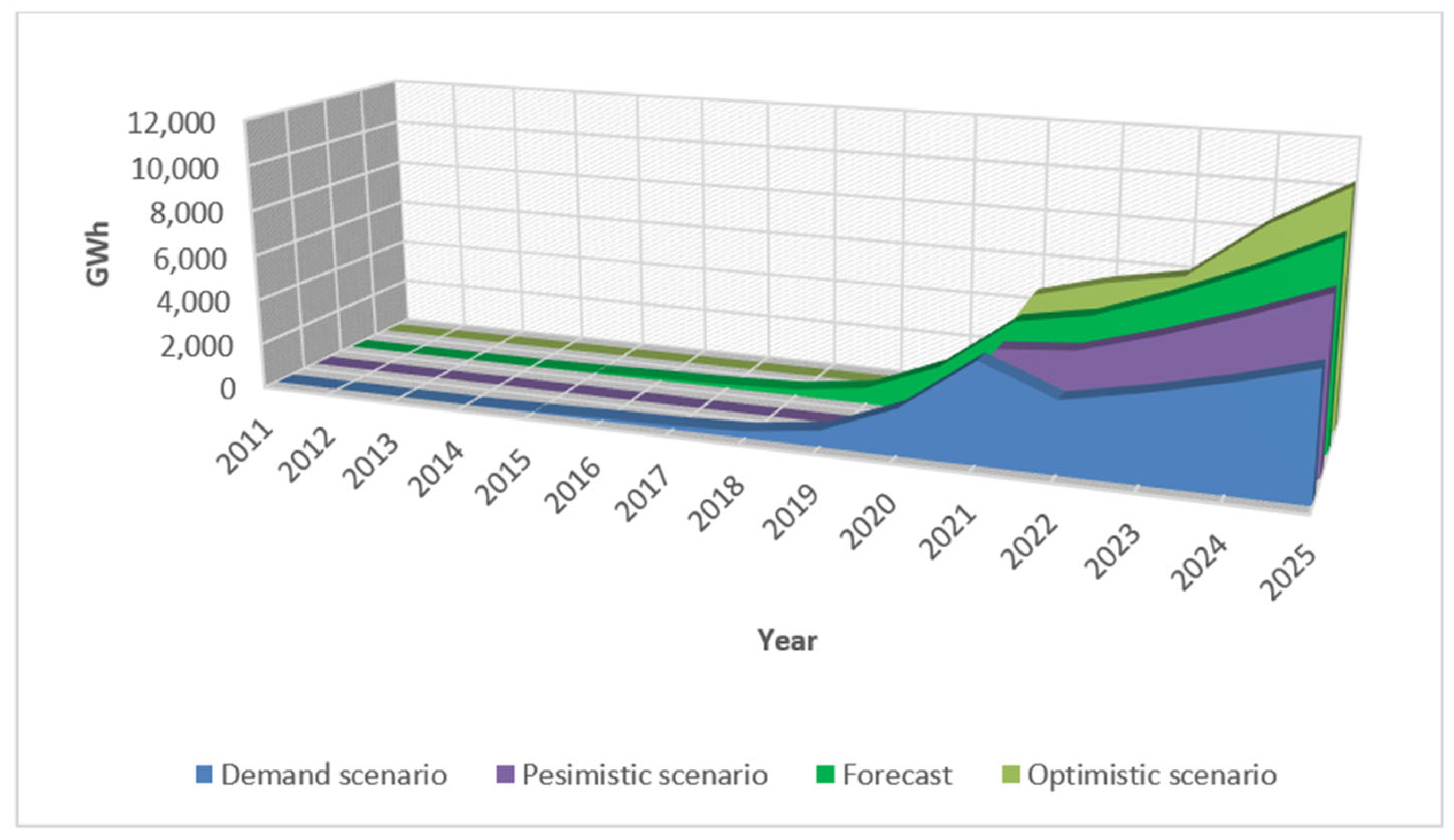
The trends shaping the explanatory variables were determined on the basis of historical data. Since there is no certainty that these variables will continue to develop in the same way in the future, it was necessary to build a confidence interval for the forecast. This is the range within which the forecast value of PV generation can move with a probability of 90%, so there is a 5% probability of 5% error for this assumption.
The built model allowed for the determination of three scenarios for the size of PV power generation until 2025:
The most likely scenario—forecast;
Pessimistic scenario—determined by the lower range of the 95% confidence interval of the model;
The optimistic scenario—plotted by the upper range of the 95% confidence interval.
The confidence coefficient can be interpreted as the probability of determining the range within which the actual value of PV power generation may fluctuate. It allows to express the uncertainty related to the forecast [
58]. The confidence interval is the interval in which the condition:
P = 1 − α is met. Typically, this probability is assumed to be 0.95, 0.99, and 0.90. The confidence interval determined that PV power generation over the forecast horizon can be on average 11% higher than the forecast value and 14% lower than the forecast value.
Because the latest changes can change the demand for photovoltaic installations in Poland for a long time, an additional scenario was performed. This time, data on installed capacity reduced by 30% were introduced into the model. The forecast showed that by 2025, the volume of PV power generation on average would be 40% lower than the original forecast, as presented in
Figure 3. In the demand scenario, the PEP2040 target for 2040 would be achieved in 2034, which would also be a good result.
Renewable energy sources are a basic solution in light of the need to carry out energy transformation. The costs of building a photovoltaic installation in Poland are decreasing every year, but they are still relatively high for the average citizen. In such a case, the cost of building the installation may consume the entire annual income, without taking into account the costs of energy storage. Therefore, financial support from the state and stable laws shaping the development of photovoltaic installations in Poland will certainly be necessary. Additionally, the energy system in Poland will require modernization, which is currently unable to absorb the energy produced by existing photovoltaic installations on sunny days. Scientists are constantly working on the development of photovoltaic technology [
59,
60], thanks to which they will have an increasingly longer lifespan, the LCOE cost will be reduced, and they will also acquire aesthetic values, which may convince additional investors.
6. Conclusions
Solar energy in Poland currently covers about 5% of the country’s electricity demand. The pace of development of photovoltaic installations exceeded previous expectations and forecasts included in PEP2040. Most of these were prosumer installations which, in the face of rising electricity prices, the threat of lack of access to energy supplies, and the amendment to the RES Act coming into force on 1 April 2023, accelerated the decision to implement their investments before the law changed. The future development of photovoltaic installations will depend on economic, ecological, energy, technological, and access to critical raw materials. Furthermore, the legal factor, i.e., promoting and supporting the development of solar energy by the state, certainly influences the level of investor interest in photovoltaic installations. Legal factors were omitted from the presented analysis due to the fact that they would require qualitative analysis and the analysis carried out for the purposes of this research was a quantitative analysis. In further research, the authors will want to take into account the legal factor and conduct a qualitative analysis of the factors that influence the development of photovoltaic installations in Poland.
An Important element of the analysis was the ability to indicate the nature of the explanatory variables introduced into the multiple regression model. Only variables whose significance was confirmed by a statistical test, and which were significant at the level of α = 0.05 and α = 0.01, were left in the model. Particular attention should be paid to those independent variables that have been identified as destimulants, because an increase in their value will signal an upcoming decline in PV power generation volume. Tracking the so-called weak signals (course of explanatory variables of time series) can provide advance information about changes in PV energy generation. The use of scenario planning is helpful in this respect, an example of which is also presented in this publication. The forecast, despite the omission of 2022 from the input data, showed that intensive increases in PV energy production in Poland can be expected by 2025. To make this possible, it is necessary to maintain the favorable trend of the explanatory variables; otherwise, the share of photovoltaic power in the total energy production in Poland may decrease. This would be unfavorable considering the need to change the country’s energy mix. Legislative changes may significantly slow the pace of development of renewable energy, as was the case in Poland with respect to wind energy. The change in the electricity billing system in April 2022 also resulted in a decline in interest in photovoltaics. Time will tell whether this method of settlement will be less beneficial for prosumers, but the change itself discouraged investors from building new installations. Photovoltaic farms built by energy companies have also begun to signal that new zoning regulations may inhibit planned investments. Ultimately, the Ministry of Development and Technology guidelines were modified and relaxed, but the fact of legislative instability can affect future investment decisions of both consumers and energy companies.
The authors verified the dependence of the development of installed PV power capacity on critical raw materials. Models were built taking into account individual critical raw materials such as Cu, Si, Ge, and Ga. Each of them showed statistical significance, which means that access to critical raw materials in the future will have a significant impact on the further development of photovoltaic installations. Currently, most of the panels used in Poland are produced in China. Since Poland is not the only country that is taking intensive steps to modify the energy mix, and thus, increase the share of solar energy in the energy generation structure, the access to raw materials necessary to produce photovoltaic technology may be limited in the future.
The energy security of EU countries, including Poland, will in the near future depend on the ability and efficiency of the country to carry out the energy transition. The European Green Deal, in line with PEP2040, assumes that this transformation will be based on renewable energy sources. These include primarily water, wind, and solar energy. In recent years, technologies that have been developing very dynamically in Poland include wind turbines and photovoltaic installations. The share of solar energy in total electricity production in Poland has increased from 0% to approximately 5% over the last 10 years. According to the forecast obtained by the authors, if the volume of electricity production does not change, this share will increase to 11% by 2030. This is in line with the Institute for Renewable Energy forecasts. According to both, in 2025 the installed capacity in Poland may amount to approximately 20 GW.
Together with energy obtained from other renewable sources and assuming that clean coal combustion will provide stabilizing support to the energy system during the transition period, Poland’s energy security should be maintained. Furthermore, valuable elements obtained from coal combustion byproducts, such as REE, can support the energy transition. REEs are essential to build wind turbines and batteries necessary to store renewable energy.


