Abstract
The performance of transformers directly determines the reliability, stability, and economy of the power system. The methodologies of minimizing the transformer manufacturing cost under the premise of ensuring performance is of great significance. This paper presented an innovative multi-objective optimization model to analyze the relationship between design parameters and transformer indicators. In addition, the sensitive analysis is conducted to exploit the interaction relationships between design parameters and targets. The reliability of the model was demonstrated in 50 MVA/110 kV and 63 MVA/110 kV prototypes, compared with the actual material usage, short-circuit impedance, and load loss, and the maximum error is less than 7%. Due to this problem having many optimization objectives and the high dimension of variables, a two-stage algorithm called MOPSO-NSGA3 (multi-objective particle swarm optimization and non-dominated sorting genetic algorithm-3) is presented. MOPSO is used to find non-domain solutions within the search space in the first stage, and the solution will be used as prior knowledge to initialize the population in NSGA3. The result shows that this algorithm can be effectively used in multi-objective optimization tasks and best meets the requirements of transformer designs that minimize the short-circuit deviation, operating loss, and manufacturing costs.
1. Introduction
Power transformers are indispensable components in power grid systems, which are widely used in power systems, rail transportation, wind power generation, and other areas [1,2,3]. However, competition among transformer manufacturers has continuously increased due to the rise in raw material prices and market globalization [4]. The methodology of transformer optimization to yield better performance with low cost has been the only route for transformer manufacturers.
Transformer design is a typical multi-objective optimization problem. Except for manufacturing costs, several factors, such as leakage impedance and temperature rise, need to be carefully handled in transformer design [5,6]. High-power laboratory data around the world show that, on average, a quarter of transformers are broken in short-circuiting tests, especially when the capacity is greater than 200 MVA [7]. The reason is mainly caused by short-circuit impact current, which will accompany huge short-circuit impact force and temperature rise in winding. Furthermore, the magnetic leakage flux will bring loss and temperature rise in other components [8,9]. Leakage impedance has a significant impact on transformer security and performance, which is the first factor that needs to be considered in transformer design. Additionally, manufacturing cost and on-load loss are other crucial factors in transformer design. As a non-convex optimization problem, the operational research method is invalid to solve. Most of the traditional transformer optimization designs are centered on a single module in the transformer [10,11,12,13,14]. Adly et al. [10] built the transformer winding model via feed-forward neural networks, and the model was optimized using a single objective optimization algorithm. Similar studies were conducted in [11,12,13,14]; the manufacturing cost, on-load loss, and winding parameters of the power transformer were separately optimized using the genetic algorithm (GA), finite element method (FEM), particle swarm optimization (PSO), and classical operations research methods. These methods can effectively optimize the specific object of the transformer but ignore the interactions between other objects, i.e., these methods lack the capacity to analyze the effect of one variable on the global. For traditional global methods [15,16], constrained multi-objective problems (CMOPS) were turned into a multi-stage single-objective optimization problem via the decomposition of the optimization objectives from top to bottom, layer by layer. Unlike other analytical methods, Orosz T built the FEM-based optimizer to optimize the leakage impedance and loss of the two-winding transformer [17]. These methods ignore the coupling relationship between the optimization objectives, and only basic feasible solutions can be obtained. Secondly, due to the top-down hierarchical constraints of the solution set, once a feasible solution cannot be obtained for a certain objective, the parameters need to be updated layer by layer, which is less robust. These methods have a complete theoretical system, but only a single feasible solution can be obtained in a single execution. In addition, these algorithms do not have global search capability, and the effectiveness of the solution set is difficult to measure qualitatively and does not support massively parallel operations.
In recent years, with the improvement of computer performance, population intelligence algorithms have achieved more outstanding results in engineering problems such as complex system optimization. A genetic algorithm [18,19,20,21,22,23] was used to optimize the transformer; the variables are usually set as winding size, number of turns, resistance, core material, etc. The fitness function can be defined according to the design requirements, such as minimizing transformer losses [24], maximizing efficiency [25], or minimizing cost [26]. Particle swarm optimization (PSO) is another famous heuristic optimization algorithm and is widely used in transformer optimization [27,28]. PSO algorithm [29,30] has a faster convergence speed and better global search capability compared with traditional heuristic algorithms.
The optimized function is mainly built based on the principal structure relationship using analytical, numerical equations [31,32,33]. These methods are easy to carry out and support massively parallel operations; however, as a linear model, it may lack the ability to fit non-linear relationships. To solve this problem, population intelligence algorithms and deep learning models were used to design and optimize the transformer. The object equation was built based on deep learning models, [34] such as the neural network (NN) and population intelligence algorithms [35,36], and was used to solve this “black box” function. This method is sample-oriented, but the optimization results are highly dependent on sample validity and diversity. In addition, engineering samples are sometimes time-consuming and costly.
The above methods are effective when the optimization object is single. But in actual engineering, optimization targets usually have multiple and even exist confrontations and conflicts. The multi-objective optimization technique [37,38,39] is an optimization method for solving multiple objective functions that can effectively solve multi-objective optimization problems. The multi-objective optimization technique can effectively solve the structural parameters of the transformer to meet the performance requirements of the transformer, such as high efficiency, low loss, low noise, etc. Many scholars have presented transformer optimization designs along these lines; their ideas can be broadly summarized as the following steps: Firstly, a multi-objective optimization model is established for transformers based on the analytical method with transformer loss, quality, and impedance as the optimization objectives according to the product characteristics. Secondly, the corresponding multi-objective optimization algorithm is used to solve the problem. Most of the mainstream multi-objective optimization models are performed based on transformer electrical design schemes, and the feasible solutions obtained by them cannot be used for structural design. In this paper, multi-objective optimization equations considering transformer impedance, mass, core section, and losses will be established according to the actual situation. In addition, the reliability of the mainstream transformer multi-objective optimization model is highly dependent on the confidence level and the accuracy of the solution algorithm. However, due to the nonconvex nature of the multi-objective optimization equations and the coupling relationship existing in each optimization objective, it is hard to obtain an ideal solution. It is difficult to evaluate the validity and convergence of the solution set once the parameters are not set correctly, and it is straightforward to fall into the local optimal solution. As the number of objectives increases, the solution space of the optimization problem grows exponentially, which makes the solution of the optimization problem very difficult and quickly generates the “dimensional disaster” problem. To address the above problems, this paper will improve the traditional NSGA algorithm by introducing adaptive weights to improve the global search capability of the model to avoid falling into a local optimum and effectively optimize the performance parameters of the transformer.
This paper can be summarized in the following parts: (1) The multi-objective optimization model is built and validated in Section 2. The sensitive analysis is used to exploit the interaction relations between design parameters and targets (2) An improved hybrid algorithm called MOPSO-NSGA3 is present in Section 3. (3) The LZDT problems were utilized to test the performance of the present algorithm in Section 4. (4) The present algorithm was utilized to optimize the transformer with 110 kV/50 MVA electrical specifications in Section 5.
2. Model Building
The transformer works on the principle of electromagnetic induction. The induced voltage U can be calculated via a well-known electromagnetic induction formula:
where Bm is the peak flux density, N is the turns of the winding, f is the frequency of the current, and Afe is the sectional area of the transformer core.
where J is the winding current density; is the conductor section area of the low-voltage winding; R is the radius of the core; f0 is the effective section coefficient which is the ratio of the filling area of the silicon steel sheet to the area of the external circle.
2.1. Impedance Analysis Equation
Short-circuit impedance, as the most critical parameter in the transformer, directly determines the current in short-circuit conditions. The short-circuit impedance value below or above a specific required value will increase the transformer manufacturing cost. The transformer will bear more short-circuit current and impact force if the impedance value exceeds the standard value. To reduce the current density in the winding, an increase in material usage will be inevitable. On the other hand, an excessive impedance will lead to excess magnetic fluxes through the winding and structural parts, which will greatly increase the overall load loss and temperature rise in the transformer.
The leakage reactance in two winding transformers can be calculated via the Rogowski method [40,41,42]:
where is the volt per turn; is the mean height of the high-voltage winding and low-voltage winding; is the equivalent height of the transformer; is the permeability under vacuum. T1, T2, and Tog are the effective breadths of low-voltage winding, clearance, and high-voltage winding; D1, D2, and Dg are the corresponding mean diameter sizes of low-voltage winding, clearance, and high-voltage winding, respectively. KR is the Rogowski factor.
The optimization objective is to minimize the deviation between requirements and calculations, set the above design parameters as θ, then the object can be written as:
where is the required short-circuit impedance which is affected by the requirement and relevant national regulations.
Once the dimension parameters are determined, the usage of copper material can be estimated via Equation (5):
where NL and Nh are the turns of high-voltage and low-voltage winding, respectively; Sl and Sha are the conductor cross-section areas of high voltage and low voltage, respectively. is the density of copper, in which to estimate the amount of copper used, the effect of the transposition of insulating paper and wires has been ignored. Once the radius dimensions are determined, according to Equation (2), the ideal core diameter is given by
where kr is the diameter magnification factor to avoid core saturation and weaken transformer operating loss.
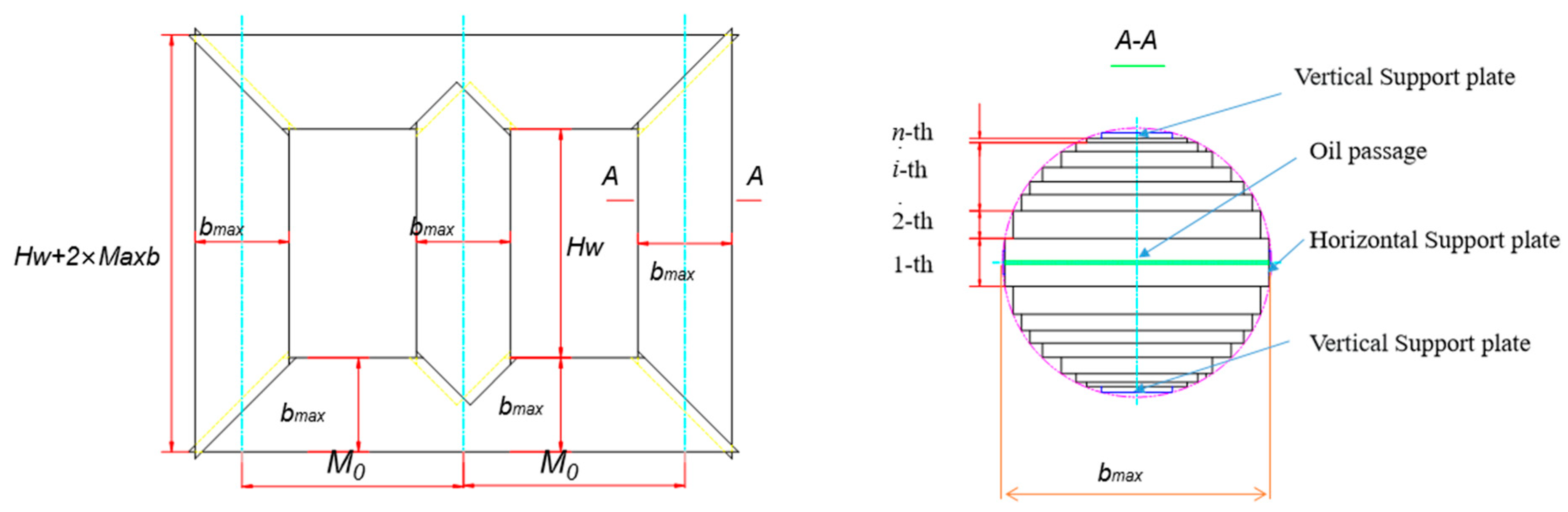
Figure 1 shows the equivalent diagram of the transformer core under the given diameter R, the transformer core is stacked with n-grade silicon steel sheets to decrease the iron loss. Mo, Hw, and bmax are the distance between phases, the height of the window, and the maximum stage width.
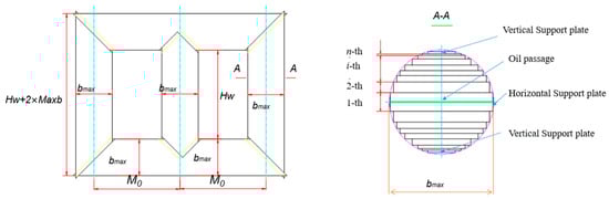
Figure 1.
Core Stacking diagram.
As shown in Figure 1, the core is filled by laminations with n step, and considering requirements of fixing and positioning, the distance must be reserved in the x and y directions and the effective area of section Sac is less than the area of the circumscribed circle with the given diameter D. To maximize the effective core area, the width of the laminations at the 1-th step and n-th step must be 0.95R and 0.2R. If it is assumed that the lamination layers are linearly decreasing in length from 1-th to n-th, set the density of silicon steel as and the total usage of silicon steel can be estimated as
In the transformer design, the overall size is mainly determined by the transformer core once the dimension parameters of the core have been determined. If the length, width and height of the transformer tank are ltk, wtk, and htk, these values can be approximated as 1.35(2M0 + 2bmax), 2.4bmax and 1.1(Hw + 2bmax) in order. Setting the thickness of the tank wall, cover, button, and the density of rolled steel as δ1, δ2, δ3, and , sequentially, the amount of total rolled steel can be approximately estimated as
2.2. Transformer Loss Equation
The total loss of the transformer is composed of two parts: no-load loss and load. No-load loss is mainly caused via the transformer core and can be subdivided into eddy loss and hysteresis loss. The unit loss Pnl can be calculated by the Steinmetz equation [7] if we ignore the abnormal loss and the microscopic eddy current loss, which is given by
where t is the thickness of the lamination;
and
are the material coefficients; n is the Steinmetz coefficient.
In addition, load loss is one of the most crucial electromagnetic performance indicators of the transformer, which directly determines the power loss caused by the internal magnetic circuit and characteristics of winding under rated operating conditions. The load loss of the transformer is mainly composed of resistance loss of winding wire, additional loss of winding, eddy loss, and stray loss in structural parts.
For a three-phase transformer, the ohmic loss in each winding is given by
where r is the resistance value of wire material; is the phase current flowing through the winding, which is co-determined by winding current density J and its cross-sectional area S. ρd is the conductivity of the copper, the value is 0.02135 Ω·mm2 during the design which means the conductivity at 75 °C. It should be noted that the current density J has a strict requirement to reduce transformer short-circuit impact force due to the relationship between radial electric force and current being quadratic [8].
The leakage flux will cause an additional loss in the wires and other steel structural parts due to the leakage magnetic field. The additional loss in each winding can be estimated by introducing an additional loss coefficient :
where is the eddy current loss coefficient of the winding; is the additional loss coefficient of the winding under incomplete transposition. The above coefficients can be calculated via the following formula:
where is the thickness of each wire in the winding; and are the reactance height and area of the wire in the specialized winding. cm is the transposition coefficient of the winding, and the derivation process and common values can be found in [43].
Except for off-load loss, the stray loss of large capacity transformer can reach 30~40% of the load loss [9]. An effective method to calculate the stray loss is 3D-FEM, but it takes a large amount of time and many computing resources will be consumed. Therefore, it is unrealistic to find the optimal under massive design schemes using 3D-FEM. The leakage flux passes through the steel structural parts (clamps, steel plates, bolts, and tank walls), and there is stray loss, which is highly correlated with the transformer capacity (Sn), the size of the transformer tank (wtk, lth and htk), and leakage impedance (X). Considering the complexity of the magnetic leakage path, it is hard to obtain precision calculation results, and the exponential regression model can be built to describe the nonlinear relationship between design parameters and stray loss under a different transformer capacity SN (MVA), which is given by:
where is the correlation coefficient of influencing factors other than design parameters; b1, b2, b3, b4, and b5 are the solving terms for the design parameters, which can be calculated using the least squares method [44] and the samplings are from transformers with electrical specification 110 kV/63 MVA and 110 kV/50 MVA; X commonly means the leakage impedance of the transformer under rated conditions and the calculation can be found in Equation (3).
2.3. Model building
Combined with Formulas (1)–(14), the optimization equation can be written as a standard form for multi-objective optimization, and the corresponding descriptions of objects are shown in Table 1:

Table 1.
Description of objects.
The explanation of the design parameter can be found in Equations (1)–(13). In addition, the design parameter is constrained to within a certain interval:
where and mean the down and up bounds of the design parameter θ. The design variables are shown in Table 2. Considering that the minimum machining precision is 0.5 mm, the design parameters have been transformed the interval; for example, [70, 110] has been mapped to [140, 220], and 141 in [140, 220] represents 70.5 in [70, 110].
Table 2.
Design variables.
Except for the above interval constraint, inequality constraints exist between partial parameters to satisfy some electrical characteristics and restrictions on transportation:
where and Smax are the allowed minimum and maximum values of the core cross-section. and are the allowed maximum upper deviation and maximum lower deviation of short circle impedance; and are the upper and lower limits of core height. and are the upper and lower limits of core length.
2.4. Sensitivity Analysis
Sobol’s method [45,46] is a widely used methodology to study the influence degree of a certain key index or a group of key indexes by a certain change in related factors from the perspective of quantitative analysis. In this method, for a vector of d uncertain inputs X, the total variance f(X) is decomposed into the variance caused by first-order parameter fi(Xi) and the variance caused by higher-order interaction terms (i.e., second-order items: fij(Xi, Xj) and j-order items f1,…,k(X1, X2,…, Xj,) for j = 3,…,d):
where δ0 is the constant term. fi,j means a function of variable Xi and Xj to express the effect of interaction on the variance. The above items are pairwise orthogonal, and the decomposition condition is
Equations (16)–(18) can be rewritten as the final variance form:
Subsequently, the sensitivity is calculated according to the variance contribution of each variable. The results contain first-order, higher-order and interaction terms which represent the effect of a single independent alteration on the output, the effect of higher-order effect and interaction terms on the model, respectively. The first-order index is a direct variance-based method and is given by
where Si represents the contribution of Xi to the final variance. Each parameter’s contribution can be calculated via the above methodology. However, it should be noticed that as the variables increase, the indices show exponential growth. As shown in Equation (18), for a model with d inputs, the total number of sensitivity indices will be 2d – 1, and large computational resources will be consumed for a high dimensional system. In this engineering multi-objective optimization task, the input variables are more than ten, and the optimization number is three. It is impractical to analyze the system with a first-order index. A methodology known as the “Total-effect index” is applied to measure the whole contribution of Xi, including all interactions under any order with any other input variables; it is calculated by
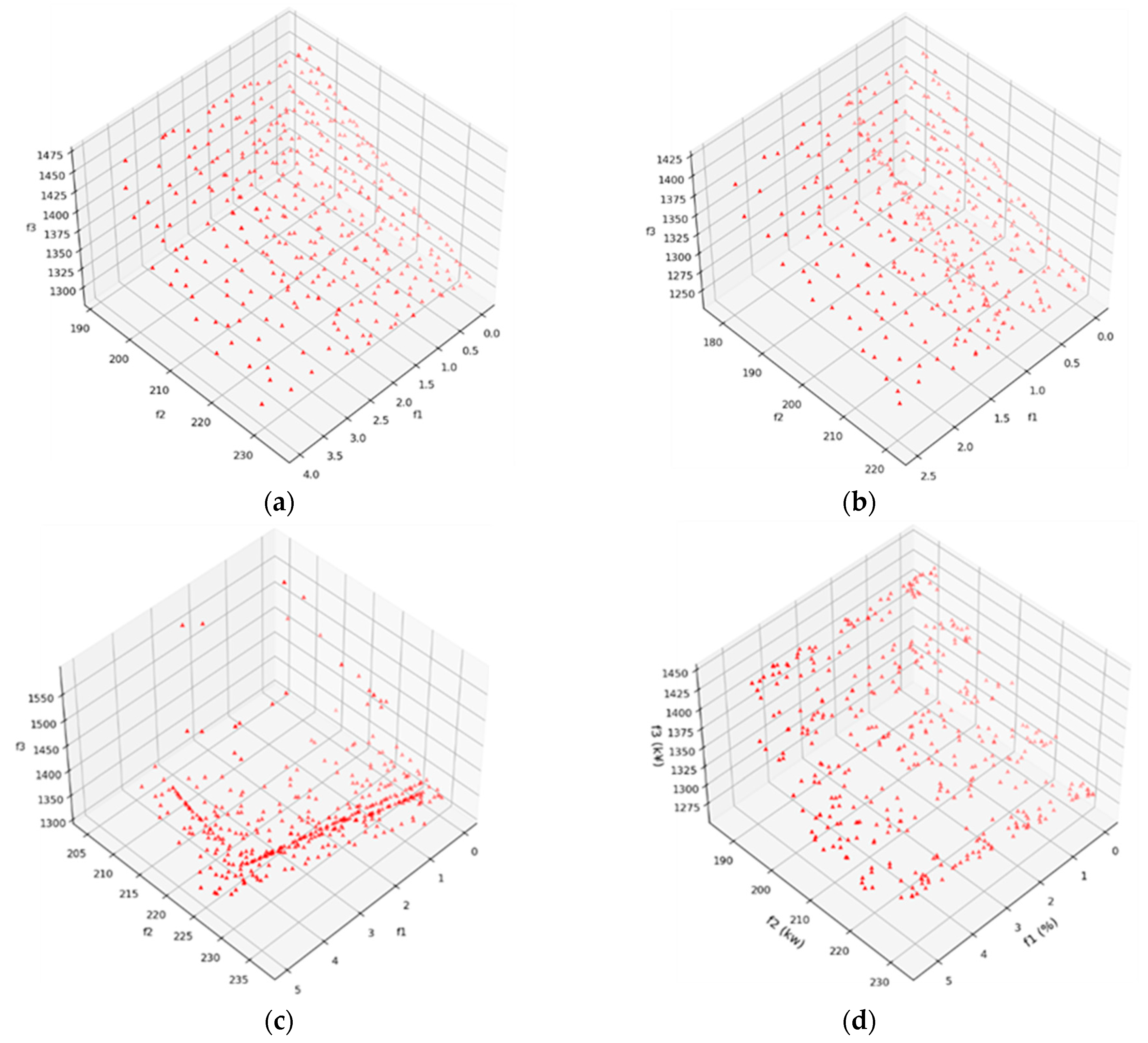
The detailed derivation process and usage cases can be found in [47]. In the response surface method (RSM), the quadratic regression model is built based on the sampling data, and analysis of variance (ANOVA) is used in causal interaction. Unlike RSM, Sobol’s sequence is calculated via Monte Carlo discretization which is adaptive under different sample sizes and valid under complex non-linear constraints. In addition, the variance-based sensitivity methods are attractive due to the sensitivity is calculated across the whole input space (i.e., global method), and widely applied in non-linear areas and non-additive systems. Figure 2 shows the total sensitivity index of the first ten items under different optimization objectives.
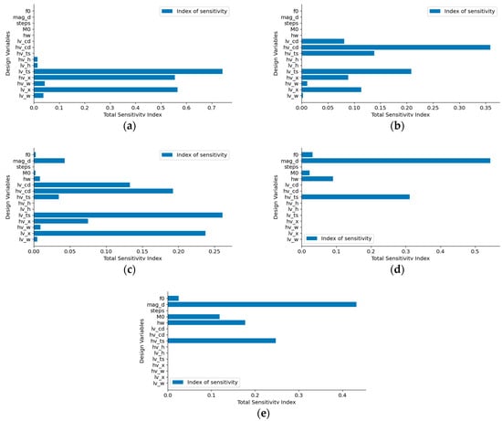
Figure 2.
Total sensitivity under different objectives. (a) Short circle impedance. (b) Copper usage. (c) Operating loss (rated operating condition). (d) Usage of silicon steel sheet. (e) Usage of steel.
In Figure 2, the sensitivity trends of each optimization objective under the same design variables are different. Once the design parameters change, it will lead to variations in these objects in different and even opposite directions. It can be found in the result that the relationships between optimization objects and variables are non-linear and even conflicted. Due to the coupling of optimization objects, there is no set of solutions to achieve the optimization of each object. The MOAs will be presented to solve this multi-objective transformer model.
2.5. Model Validating
The design details of two transformers with specification 50 MVA/110 kV and 63 MVA/110 kV has been utilized to test the accuracy of the presented model in Section 2.3. It should be pointed out the actual transformer has been put into service by several national and local grid companies. The impedance and load loss were measured via a well-known short-circuit test, and the usage of material was recorded in the cost accounting sheet. Table 3 and Table 4 show the comparison of the calculated values with the actual values for the given parameters:
Table 3.
63 MVA/110 kV.
Table 4.
50 MVA/110 kV.
In Table 3 and Table 4, the maximum absolution errors between calculated values and measured values exhibit different characteristics in transformers with other electrical specifications. The error can be summarized as follows: (a) The requirements of insulation mode and margin are different with the growth in voltage and capacity. In addition, as the result of sensitivity analysis in Section 2.4, the variation in coil parameters will lead to a massive fluctuation in each index, leading to the error sizes of coil axial and overall transformer size. (b) The general structure of the transformer is affected by many aspects, such as transportation mode, use environment, and user needs. (c) Due to the measured value being the actual usage of the whole manufacturing, the calculation model could be more efficient in considering processing losses and manufacturing deviation. In addition, as the result of sensitivity analysis in Section 2.4, the variation in coil parameters will lead to a massive fluctuation in each index. Generally, the maximum absolution is less than 9.24% and 7.12% in transformers with the electrical specification of 63 MVA/110 kV and 50 MVA/110 kV, respectively. This model can effectively evaluate the relationship between design parameters and the optimization objects.
3. MOPSO-NSGA-III Algorithm
3.1. MOPSO
The particle swarm optimization (PSO) algorithm is derived from the research of bird predation behavior: the function optimization process is realized by simulating the swarm intelligence behavior. Each particle has only two attributes: position xi and velocity Vi. In the epoch of t, the current fitness function is updated based on the individual historical best and the swarm best . Multi-objective particle swarm optimization (MOPSO) has a similar process flow to the PSO algorithm. The best history position of the swarm can be directly located via fitness value in PSO. The Pareto domination is used to evaluate the quality of multi-objective fitness in MOPSO, and particles that are not dominated have a higher probability of being retained. The best swarm pb in the Pareto set is selected via crowding density. The swarm with low crowding density will be used to update the velocity V and position P of the remaining swarm that does not belong to the Pareto set. The velocity Vi and position xi of each particle are updated via:
where C1 and C2 are the individual learning factor and the group learning factor, respectively. r1 and r2 are uniform random numbers in the interval [0, 1]. For w, which can be referred to as a constant, the linear decreasing strategy is taken in this paper:
where Tmax is the maximum iteration number; wmax and wmin are the maximum and the minimum inertia coefficient. We set wmax to 0.9 and wmin as 0.4 to ensure the algorithm has better global search ability in the early iteration and can effectively converge in the end. The flow of the algorithm at epoch t is given in Table 5.
Table 5.
Generation t of MOPSO.
Compared with other heuristics algorithms, MOPSO is more straightforward to implement. The MOPSO algorithm only needs to initialize the position and speed of individual particles and optimize the search through simple iterative updating rules. In addition, MOPSO has advantages in global search capability. The particle updates its velocity and position to find the global optimal solution. With the help of information sharing and cooperation between particles, it can converge to the global optimal solution quickly. The randomized policy is taken to choose the pb as shown in step (6) of Table 5. This strategy is significant in enlarging the search scopes and overcoming premature convergence. However, it should be noted that the search accuracy will be weakened in each search target. Hence, the other multi-objective optimization algorithm will be utilized to refine the optimization based on the solutions of the presented MOPSO. The solutions obtained by MOPSO will be applied as the prior knowledge to initialize the population in NSGA3.
3.2. NSGA-III Algorithm
The main idea of NSGA3 is to introduce the reference point mechanism based on NSGA2 to retain those individuals that are not dominated and close to the reference point. In general, NSGA3 and NSGA2 have a similar framework, and the main difference is the selection mechanism change. NSGA2 mainly relies on crowding degree to sort, which is unsuitable in high-dimensional objective space. NSGA3 makes a dramatic adaptation to the crowding degree sort and introduces widely distributed reference points to maintain the diversity of the population. More details of the implementation can be found in [48]. The algorithm flow of generation t is given in Table 6.
Table 6.
Generation t of NSGA3.
The operation of crossover, selection, and mutation in step (2) from Table 6 is the same as the common genetic algorithm, and the coding scheme is decided according to the problem. In this optimization case, the binary encoding is used for each integer variable, and the actual encoding is used for the other variables. Unlike single objective optimization, the fitness can be directly decided via the function value. The difficulty of the heuristic multi-objective optimization algorithm is how to maintain the population, ensure the global search ability of the algorithm, and select N object from the whole number of the population with the length of 2N. The fast non-dominated sorted algorithm is utilized to divide the population into different groups ND via the dominated rank. The population from ND with the dominated rank lower than l will be selected as the next generation. When the corresponding number is the same as the N, the population in generation t is confirmed, but in more cases, K populations are still needed to constitute the next generation population. The crowding degree ranking strategy is taken in NSGA2 to screen out the better population with the same dominance level. However, this methodology has high computational complexity, and its effect could be more evident in high-dimensional problems. Population diversity is maintained, and algorithm complexity is decreased in the NSGA3 compared with the NSGA2 by introducing widely distributed reference points. Although compared with the NSGA2 algorithm, the NSGA3 algorithm effectively reduces the computational complexity and improves the global search ability of the algorithm. However, the solution process is still highly dependent on the initial solution set and initialization parameters. The performance and effect of NSGA3 are closely related to its parameter settings. For example, the number and distribution of reference points, the parameters chosen by the environment, etc., impact the algorithm’s operation. Incorrect parameter settings may lead to the degradation of the solution set quality or the local optimal solution. Eventually, consistent with the vast, well-known multi-objective algorithms, the ideal solution set takes a lot of work to achieve for high dimensional optimization objectives. The repeated execution of a single algorithm is unable to maintain the global search ability of the solution.
3.3. MOPSO-NSGA3 Hybrid Algorithm
MOPSO and NSGA-III are well-known methods widely used in multi-objective engineering tasks. However, using only a single algorithm for MOPs will cause drawbacks such as insufficient search space and non-convergence of a final solution set. Due to the limitations of a single algorithm, the two-stage joint optimization algorithm named MOPSO-NSGA3 is presented to optimize the mentioned engineering optimization question. The workflow of MOPSO-NSGA3 is shown in Figure 3. In MOPSO-NSGA3, the advantages of global searching ability from MOPSO and escaping from local optimal from NSGA3 are taken to improve the algorithm’s overall performance. MOPSO is used in the first stage to perform a global search. The random factor is taken in the global optimal selection mechanism of the MOPSO algorithm, which is utilized to enlarge the searching space and find the potentially excellent non-dominated points. According to the “No free lunch” theory, this strategy will inevitably weaken the searching precision and global convergence of the algorithm. The NSGA3 will be used as a two-stage algorithm in the next step. The final particle swarms will be utilized as the prior experience population and the NSGA3 will be executed based on existing search results. As a heuristic algorithm, the initialized population directly determined the quality of the final Pareto solutions. This strategy will strengthen the search efficiency of the NSGA3 algorithm in the early stage and avoid the problem of falling into the local optimum caused by the poor quality of the initial population.
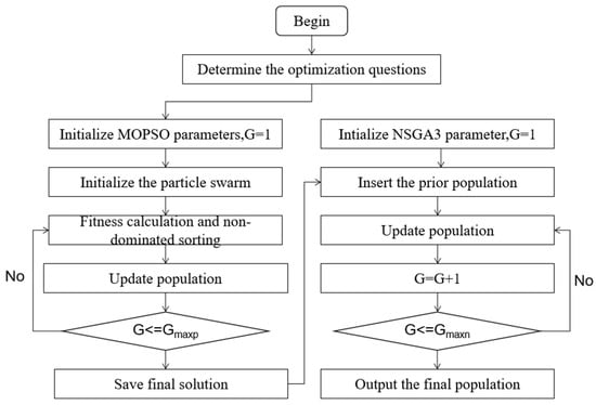
Figure 3.
Flow of MOPSO-NSGA3 algorithm.
In Figure 3, the flow of the algorithm is divided into two parts: MOPSO and NSGA3. In MOPSO, the swarms are randomly initiated in the range, as shown in Table 2. The individual learning coefficient c1 and social learning coefficient c2 are set as 1 and 2 to enlarge the search space. It should be noted that several changes have been applied in the present MOPSO to meet the needs of the hybrid algorithm, which is specifically used for searching the potential front Pareto sets in the first stage. After the processing of MOPSO, the final swarms will be utilized as the initial population in NSGA3 by setting the same population size. The widely distributed reference point is introduced in the NSGA3 as a modification of the selection mechanism. The algorithm is more suitable for multi-objective problems with high dimensions compared with NSGA2. Details of procedures are shown in Table 6.
4. Experimental Test
In this chapter, a series of benchmark tests will be carried out to measure the global search ability and solution set convergence of the presented MOPSO-NSGA3 algorithm. In addition, the well-known MOPSO, NSGA2, and NSGA3 will be tested to make a horizontal contrast with the present methodology. The hyperparameters of each algorithm are set to the same specification to ensure the reliability of the test results.
Comparison of Results of Different Optimization Algorithms
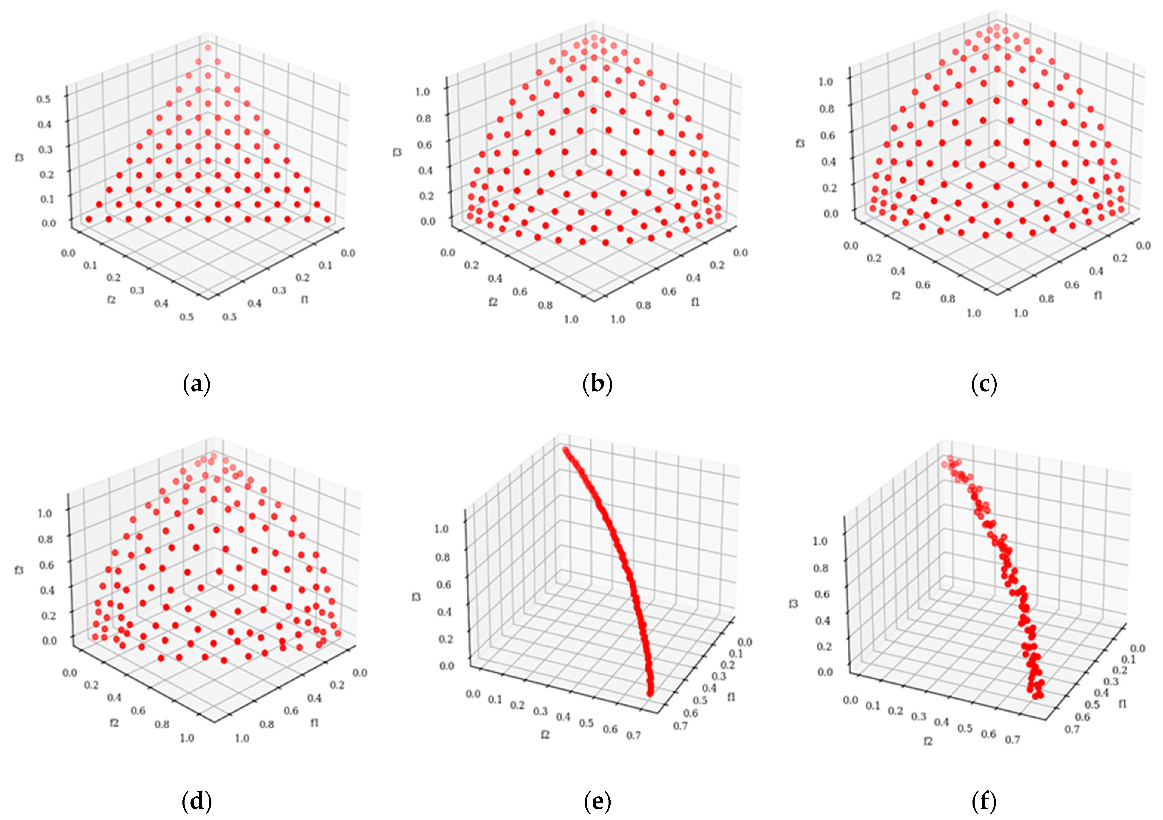
In this section, the DTLZ problems will be utilized to evaluate the convergence and global search ability of each algorithm. For the presented MOPSO-NSGA3, in MOPSO, the iterations Gmax and population number are set as 100 and 200, respectively. After the first stage, the swarms in MOPSO will be applied as the prior population. Therefore, the population is the same as MOPSO and set as 200. The crossover rates are set as linearly decreasing. The maximum and minimum are pmax = 0.5 and pmin = 0.05, respectively. DTLZ1 is a classical benchmark problem with a linear Pareto optimal plane, and its complexity increases linearly with the number of independent variables. This problem can effectively evaluate the global convergence of the algorithm under the high latitude problem. DTLZs (2)–(4) further increase the difficulty of algorithm optimization by adding linear transformation to the independent variables based on DTLZ1. DTLZs (1)–(4) can effectively evaluate the ability of a multi-objective optimization algorithm to converge to a specific plane to a certain extent. However, the optimal plane usually presents non-specification geometric plane characteristics in practical engineering problems. Therefore, the convergence was changed to a spatial curve in DTLZ5-6 to test the performance of the function to converge to a specific curve. Figure 4 shows the final front Pareto set achieved by MOPSO-NSGA3. The expression equations and details of DTLZ (1)~(6) can be found in [44].
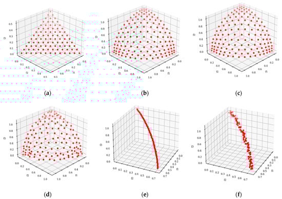
Figure 4.
Pareto points obtained by present MOPSO-NSGA3 under DTLZs: (a) DTLZ1. (b) DTLZ2. (c) DTLZ3. (d) DTLZ4. (e) DTLZ5. (f) DTLZ6.
Table 7 shows the items HVmean, IGDmin, IGDmax, and IGDmean, which mean, respectively, the mean value of HV, the minimum, maximum, and mean value of IGD. Each MOA has been run 20 times for each problem to weaken the random fluctuations in the heuristic algorithm. The best value is highlighted in bold. HV is a widely used comprehensive evaluation index and can be easily calculated via the ND set. Generally, a significant numerical value represents the strong convergence, spread, and diversity of the final ND sets and vice versa. In most cases, the present MOPSO-NSGA3 algorithm shows better performance in the indicator of HV, except DTLZ2, compared with other algorithms. The HV indicator can evaluate the performance of the MOAs in some way; it is unable to assess the difference between actual Pareto front PF* and obtained Pareto ND sets. DTLZ is a series of benchmark problems to evaluate the ability of MOAs to converge to a known plane. As shown in Table 7, the ND solutions from our presented methodology achieved the minimum value in the indicators of IGDmax, IGDmean, and IGDmin for all DTLZ problems. The indicator of IGDmean shows the ND set achieved by MOPSO-NSGA3 is close to the PF* compared with other MOAs. In addition, combined with results in the indicators of IGDmax and IGDmin, it can be found the present solution has better stability and robustness in all kinds of situations.
Table 7.
The performance of five MOEAs for six DTLZ problems.
The results of the benchmark test show the MOPSO-NSGA3 algorithm can effectively handle MOPs with different constraints and approximate specific true Pareto front (PF*) plane. In addition, the distribution, validity, and consistency of the ND set obtained by the present method are proved in the indicators of HV and IGD. In this chapter, the comprehensive performance of the present algorithm is validated via a benchmark test and shows the best performance compared with popular MOAs. The following section will utilize the proposed hybrid algorithm to optimize the transformer.
5. Optimization
The convergence and global search capability has been proven in Section 4. Unlike benchmark tests, the IGD cannot calculated due to the unknown of true Pareto front PF*. It is hard to find the optimal ND set without designer preference in multi-objective problems. Therefore, this paper will evaluate the performance of each algorithm based on the comprehensive index of the final solution set.
Result Comparisons
Except for the present algorithm, the three mentioned algorithms are also utilized to optimize the current problems, and the distribution and domination relations of the final Pareto set of each algorithm are compared and analyzed. The prototype electrical specifications of the transformer to be optimized is 50,000 kVA/110 kV, and details can be found in Table 8. It should be noted that the mentioned transformer is a company’s regular product and has been widely applied in the power system. The description of the optimization model and design parameter is listed in Section 2. The population of each algorithm and iteration times have been set as 400 and 200, respectively, considering the large number of variables. The crossover rate is dynamic, linearly decreasing in weight. The minimum and maximum crossover rates are set as 0.5 and 0.05, respectively for NSGA2 and NSGA3. The polynomial mutation probability is set as 1/D, where D is the number of variables. The final solutions obtained by each algorithm are given in Figure 5. The corresponding mean, minimum, maximum, and standard deviation values of each objective in the Pareto solution are shown in Table 9.
Table 8.
Design requirement.
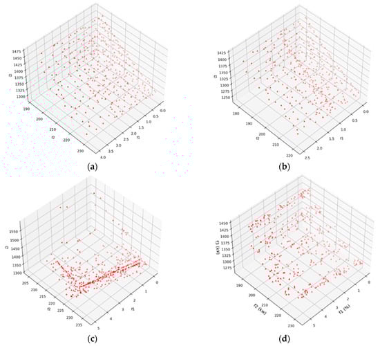
Figure 5.
Pareto fronts achieved by MOAs: (a) NSGA2. (b) MOPSO-NSGA3. (c) MODE. (d) NSGA3.
Table 9.
Comprehensive performance of each algorithm.
In Figure 5, the cost of transformer f3 and its operating loss f2 show an opposite trend under each algorithm; that is, for the sake of decreasing loss, the effective methods are increasing coil cross-section and reducing design magnetic density, which will dramatically increase the usage of raw materials and manufacturing cost. The material cost of the final solution obtained via MOPSO-NSGA3 is obviously reduced compared with the other algorithm without the deterioration of other indicators. The short-circuit impedance deviation f3 is mainly affected by the lateral and radial dimensions of the coil. Considering the errors from machining and assembly, this indicator needs to be as small as possible. The short-circuit impedance deviation of the present MOPSO-NSGA3 algorithm can be restricted to 3%, compared with other MOAs that can better adapt to actual needs. The comprehensive performance of each algorithm can be found in Table 9.
The mean, minimum, and maximum values of the three objects have been listed in Table 8, and the best values of the four algorithms have been marked in bold. In most cases, the presented algorithm achieved the best performance under the indicators of Avg, Min, and Max. Figure 5d the solution is uniformly distributed in the space, which can best fit the needs under different design requirements compared with other mainstream MOAs. The dominated numbers in the solutions of the present algorithm, NSGA2, NSGA3 and MOPSO are 0, 21, 0, and 147, respectively. The Std indicator is used to evaluate the distributivity of each algorithm to some degree, but when the solution set does not converge and existing dominated individuals, the value will lack reference. According to the previous analysis, the conclusion can be achieved that the present algorithm can best satisfy the transformer design under different requirements among the MOAs.
6. Conclusions
This paper presented a hybrid multi-objective algorithm called MOPSO-NSGA3 to minimize the deviation of short-circuit, transformer loss, and manufacturing cost. The result showed the present methodology can achieve better Pareto solutions to fit the different requirements of design compared with NSGA2, NSGA3, and MOPSO. Additionally, the related research has been carried out:
- (a)
- The multi-objective optimization model was built, and the accuracy model was validated via two transformers with the electrical specifications of 110 kV/50 MVA and 110 kV/63 MVA.
- (b)
- Sensitive analysis was carried out to analyze the interaction relationship between transformer design parameters and each optimization object.
- (c)
- The optimization work of the transformer with 110 kV electrical specifications has been carried out.
However, several works need to be carried out due to the nonlinear relationships between design parameters and optimization objects. The following works can be summarized as the following way:
- (a)
- The analytical method was utilized to calculate short-circuit impedance in this paper, but this method is insufficient to consider the affections of material nonlinearity and core saturation characteristics. However, the finite element method is time-consuming and accompanied by a large computational quantity, which is unrealistic to operate in massively parallel computing. The lightweight machine learning (LN) and deep learning (DL) models will be used as the object function in the future to decrease the error from model prediction.
- (b)
- The flux leakage control, insulation requirements, and heat-dissipating method differ sharply for transformers with different voltage levels and operating capacities. The present multi-objective model needs to be improved to cover other types of transformers.
Author Contributions
Conceptualization, L.Z. and Z.L.;Project administration, L.Z. Software, B.S., W.X. and J.S., Methodology, B.S.; Writing—review and editing, Y.J. and Z.L.; Investigation, L.Z., X.C. and J.S. Visualization, Y.J. and W.X.; Writing—original draft, B.S. Validation, X.C and L.Z. Data curation, M.L. and Z.L; Formal analysis, L.Z. and Z.L. All authors have read and agreed to the published version of the manuscript.
Funding
The authors would like to thank the financial support from the National Natural Science Foundation of China (No. 51879089) and China XD Group Research Project (No. XDCB2023KJ001).
Data Availability Statement
Data are contained within the article.
Acknowledgments
The authors would like to thank anyone who wants to make this paper better. The authors would like to thank the financial support from the National Natural Science Foundation of China (No. 51879089) and China XD Group Research Project (No. XDCB2023KJ001).
Conflicts of Interest
Authors Baidi Shi, Liangxian Zhang, Zixing Li, Wei Xiao, Xinfu Chen and Meng Li were employed by the company Changzhou Xidan Transformer Co., LTD. The other authors declare no conflict of interest.
Abbreviations
| U | Induced voltage | Equivalent magnetic leakage area | |
| f | Current frequency | Equivalent reactance height | |
| Bm | Peak flux density | T1 | Breadth of low-voltage winding |
| Afe | Sectional area of the core | T2 | Breadth of high-voltage winding |
| R | The radius of the core | Density of rolled steel | |
| N | Turns of the Winding | Tg | Breadth of clearance |
| SN | Transformer rated capacity | D1 | mean diameter size of low-voltage winding |
| f0 | Effective section coefficient | D2 | mean diameter size of high-voltage winding |
| KR | Rogowski factor | Dg | mean diameter size of clearance |
| Required short-circuit impedance | X | Short-circuit impedance | |
| Density of copper | Turns of low-voltage winding | ||
| Turns of high-voltage winding | Sl | Conductor cross-section area of low-voltage winding | |
| SH | Conductor cross-section area of high-voltage winding | Density of silicon steel | |
| Effective cross-sectional area of the core | bmax | Maximum stage width of core | |
| bmin | Minimum stage width of core | Height of the window | |
| Length of the tank | Width of the tank | ||
| Height of the tank | δ1 | Thickness of tank wall | |
| δ2 | Thickness of tank cover | δ3 | Thickness of tank bottom |
| Unit loss of silicon steel | Thickness of the core lamination | ||
| Eddy loss | Additional loss coefficient | ||
| b1~b5 | Stray loss regression coefficient | k1, k2 | Material dependent coefficients |
| hysteresis loss | Eddy loss coefficient of winding | ||
| Additional winding loss coefficient | Pnl | No-load loss | |
| Stray loss of the transformer | Winding resistance loss | ||
| cm | Transposition coefficient of winding | Variance of variable i | |
| First-order sensitivity of variable i | Total sensitivity of variable i | ||
| PSO | Particle swarm optimization | NSGA | Non-dominated sorting genetic algorithm |
| MOA | Multi-objective algorithm | MOP | Multi-objective problem |
| MO | Multi-objective | GA | Genetic algorithm |
References
- Georgilakis, P.S. Transformer Design Optimization. Power Syst. 2009, 38, 331–376. [Google Scholar]
- Ćalasan, M.P.; Jovanović, A.; Rubežić, V.; Mujičić, D.; Deriszadeh, A. Notes on Parameter Estimation for Single-Phase Transformer. IEEE Trans. Ind. Appl. 2020, 56, 3710–3718. [Google Scholar] [CrossRef]
- Cai, Z.; Zha, C.; Zhan, R.; Huang, G. Analysis and calculation of magnetic flux density distribution and core loss of nanocrystalline transformer. Energy Rep. 2022, 8, 218–225. [Google Scholar] [CrossRef]
- Li, S.; Sun, F.; Li, M.; Wang, C.; Li, X.; Yuan, P.; Zeng, H. The Research of 220kV Transformer Optimization Design Based on Finite Element Analysis Method. In Proceedings of the 2019 Chinese Automation Congress (CAC), Hangzhou, China, 22–24 November 2019; Institute of Electrical and Electronics Engineers Inc.: Piscataway, NJ, USA; pp. 5800–5803. [Google Scholar]
- Qin, J.; Yang, D.; Wang, N.; Ni, X. Convolutional sparse filter with data and mechanism fusion: A few-shot fault diagnosis method for power transformer. Eng. Appl. Artif. Intell. 2023, 124, 106606. [Google Scholar] [CrossRef]
- Zou, D.; Xiang, Y.; Zhou, T.; Peng, Q.; Dai, W.; Hong, Z.; Shi, Y.; Wang, S.; Yin, J.; Quan, H. Outlier detection and data filling based on KNN and LOF for power transformer operation data classification. Energy Rep. 2023, 9, 698–711. [Google Scholar] [CrossRef]
- Hernandez, A.; Canedo, J.M.; Olivares-Galvan, J.C.; Betancourt, E. Novel technique to compute the leakage reactance of three-phase power transformers. IEEE Trans. Power Deliv. 2016, 31, 437–444. [Google Scholar] [CrossRef]
- Kulkarni, S.V.; Khaparde, S.A. Transformer Engineering Design and Practice, 2nd ed.; CRC Press: New York, NY, USA, 2017. [Google Scholar]
- Dawood, K.; Kmirgz, G. A simple analytical method foraccurate prediction of the leakage reactance and leakage energyin high voltage transformers. J. King Saud Univ. Eng. Sci. 2022, in press. [Google Scholar] [CrossRef]
- Adly, A.A.; Abd-El-Hafiz, S.K. Automated transformer design and core rewinding using neural networks. J. Eng. Appl. Sci. 1999, 46, 351–364. [Google Scholar]
- Georgilakis, P.S. Recursive genetic algorithm-finite element method technique for the solution of transformer manufacturing cost minimization problem. IET Electr. Power Appl. 2009, 3, 514–519. [Google Scholar] [CrossRef]
- Hernández, C.; Arjona, M.A. Design of distribution transformers based on a knowledge-based system and 2D finite elements. Finite Elem. Anal. Des. 2007, 43, 659–665. [Google Scholar] [CrossRef]
- Hengsi, Q.; Kimball, J.W.; Venayagamoorthy, G.K. Particle swarm optimization of high-frequency transformer. In Proceedings of the 36th Annual Conference on IEEE Industrial Electronics Society (IECON), Glendale, AZ, USA, 7–10 November 2010; pp. 2914–2919. [Google Scholar]
- Tsili, M.A.; Kladas, A.G.; Georgilakis, P.S. Computer aided analysis and design of power transformers. Comput. Ind. 2008, 59, 338–350. [Google Scholar] [CrossRef]
- Balci, S.; Sefa, I.; Altin, N. Design and analysis of a 35 kVA medium frequency power transformer with the nanocrystalline core material. Int. J. Hydrogen Energy 2017, 42, 17895–17909. [Google Scholar] [CrossRef]
- Gu, S.; Han, L.; Liu, D.; Yu, W.; Xiao, Z.; Feng, T. Design and applicability analysis of independent double acquisition circuit of all-fiber optical current transformer. Glob. Energy Interconnect. 2019, 2, 531–540. [Google Scholar] [CrossRef]
- Orosz, T. FEM-Based Power Transformer Model for Superconducting and Conventional Power Transformer Optimization. Energies 2022, 15, 6177. [Google Scholar] [CrossRef]
- Janjua, A.K.; Mughal, S.N.; Khan, A.Z. Transformer’s Core Size Optimizaiton Using Genetic Algorithm. Conference Transformer’s Core Size Optimizaiton Using Genetic Algorithm. In Proceedings of the 2015 6th International Conference on Intelligent Systems, Modelling and Simulation, Kuala Lumpur, Malaysia, 9–12 February 2015; pp. 179–183. [Google Scholar]
- Marinov, A.; Bekov, E.; Feradov, F.; Papanchev, T. Genetic Algorithm for Optimized Design of Flyback Transformers. In Proceedings of the Conference Genetic Algorithm for Optimized Design of Flyback Transformers, Bourgas, Bulgaria, 3–6 June 2020; pp. 1–4. [Google Scholar]
- Shintemirov, A.; Tang, W.H.; Wu, Q.H. Construction of transformer core model for frequency response analysis with genetic Algorithm. In Proceedings of the Conference Construction of Transformer Core Model for Frequency Response Analysis with Genetic Algorithm, Calgary, AB, Canada, 26–30 July 2009; pp. 1–5. [Google Scholar]
- Zhang, S.; Hu, Q.; Wang, X.; Zhu, Z. Application of Chaos Genetic Algorithm to Transformer Optimal Design. In Proceedings of the Conference Application of Chaos Genetic Algorithm to Transformer Optimal Design, Shenyang, China, 6–8 November 2009; pp. 108–111. [Google Scholar]
- Zheng, R.R.; Zhao, J.Y.; Wu, B.C. Transformer Oil Dissolved Gas Concentration Prediction Based on Genetic Algorithm and Improved Gray Verhulst Model. In Proceedings of the Conference Transformer Oil Dissolved Gas Concentration Prediction Based on Genetic Algorithm and Improved Gray Verhulst Model, Shanghai, China, 7–8 November 2009; Volume 4, pp. 575–579. [Google Scholar]
- Ajour, M.N.; Abu-Hamdeh, N.H.; Mostafa, M.E. Optimizing and simulating cooling of electric transformer room utilizing genetic algorithm to reduce electricity/water demand by incorporating borehole ground heat exchangers. J. Taiwan Inst. Chem. Eng. 2023, 148, 104907. [Google Scholar] [CrossRef]
- Abdelwanis, M.I.; Abaza, A.; El-Sehiemy, R.A.; Ibrahim, M.N.; Rezk, H. Parameter Estimation of Electric Power Transformers Using Coyote Optimization Algorithm with Experimental Verification. IEEE Access 2020, 8, 50036–50044. [Google Scholar] [CrossRef]
- Guo, Z.; Yu, R.; Xu, W.; Feng, X.; Huang, A.Q. Design and Optimization of a 200-kW Medium-Frequency Transformer for Medium Voltage SiC PV Inverters. IEEE Trans. Power Electron. 2021, 36, 10548–10560. [Google Scholar] [CrossRef]
- Cheema, M.A.M.; Fletcher, J.E.; Dorrell, D. A Practical Approach for the Global Optimization of Electromagnetic Design of 3-Phase Core-Type Distribution Transformer Allowing for Capitalization of Losses. IEEE Trans. Magn. 2013, 49, 2117–2120. [Google Scholar] [CrossRef]
- Fei, S.-W.; Wang, M.-J.; Miao, Y.-B.; Tu, J.; Liu, C.-L. Particle swarm optimization-based support vector machine for forecasting dissolved gases content in power transformer oil. Energy Convers. Manag. 2009, 50, 1604–1609. [Google Scholar] [CrossRef]
- Illias, H.A.; Chai, X.R.; Abu Bakar, A.H. Hybrid modified evolutionary particle swarm optimisation-time varying acceleration coefficient-artificial neural network for power transformer fault diagnosis. Measurement 2016, 90, 94–102. [Google Scholar] [CrossRef]
- Korab, R.; Połomski, M.; Owczarek, R. Application of particle swarm optimization for optimal setting of Phase Shifting Transformers to minimize unscheduled active power flows. Appl. Soft Comput. 2021, 105, 107243. [Google Scholar] [CrossRef]
- Liao, R.; Zheng, H.; Grzybowski, S.; Yang, L. Particle swarm optimization-least squares support vector regression based forecasting model on dissolved gases in oil-filled power transformers. Electr. Power Syst. Res. 2011, 81, 2074–2080. [Google Scholar] [CrossRef]
- Lren, M. Optimization of transformer parameters at distribution and power levels with hybrid Grey wolf-whale optimization algorithm. Eng. Sci. Technol. Int. J. 2023, 43, 101439. [Google Scholar]
- Kotb, M.F.; El-Fergany, A.A.; Gouda, E.A. Estimation of electrical transformer parameters with reference to saturation behavior using artificial hummingbird optimizer. Sci. Rep. 2022, 12, 19623. [Google Scholar] [CrossRef] [PubMed]
- Orosz, T.; Karban, P.; Pánek, D.; Doleel, I. FEM-based transformer design optimization technique with evolutionary algorithms and geometric programming. Int. J. Appl. Electromagn. Mech. 2020, 64, 1–9. [Google Scholar] [CrossRef]
- LeCun, Y.; Bengio, Y.; Hinton, G. Deep learning. Nature 2015, 521, 436–444. [Google Scholar] [CrossRef]
- Li, K.; Ding, Y.-Z.; Ai, C.; Sun, H.; Xu, Y.-P.; Nedaei, N. Multi-objective optimization and multi-aspect analysis of an innovative geothermal-based multi-generation energy system for power, cooling, hydrogen, and freshwater production. Energy 2022, 245, 123198. [Google Scholar] [CrossRef]
- Marghny, M.H.; Zanaty, E.A.; Dukhan, W.H.; Reyad, O. A hybrid multi-objective optimization algorithm for software requirement problem. Alex. Eng. J. 2022, 61, 6991–7005. [Google Scholar] [CrossRef]
- Shen, X.; Yu, G.; Chen, Q.; Hu, W. A multi-objective optimization co-evolutionary algorithm with dynamically varying number of subpopulations. Control. Decis. 2007, 22, 1011–1016. [Google Scholar]
- Wang, Y.; Chen, C.; Tao, Y.; Wen, Z.; Chen, B.; Zhang, H. A many-objective optimization of industrial environmental management using NSGA-III: A case of China’s iron and steel industry. Appl. Energy 2019, 242, 46–56. [Google Scholar] [CrossRef]
- Wu, X.; Li, X.; Qin, Y.; Xu, W.; Liu, Y. Intelligent multiobjective optimization design for NZEBs in China: Four climatic regions. Appl. Energy 2023, 339, 120934. [Google Scholar] [CrossRef]
- Solís-Pérez, J.E.; Gómez-Aguilar, J.F.; Hernández, J.A.; Escobar-Jiménez, R.F.; Viera-Martin, E.; Conde-Gutiérrez, R.A.; Cruz-Jacobo, U. Global optimization algorithms applied to solve a multi-variable inverse artificial neural network to improve the performance of an absorption heat transformer with energy recycling. Appl. Soft Comput. 2019, 85, 105801. [Google Scholar] [CrossRef]
- Mohammed, M.S.; Vural, R.A. NSGA-II+FEM Based Loss Optimization of Three-Phase Transformer. IEEE Trans. Ind. Electron. 2019, 66, 7417–7425. [Google Scholar] [CrossRef]
- Al-Dori, O.; Sakar, B.; Dnik, A. Comprehensive analysis of losses and leakage reactance of distribution transformers. Arab. J. Sci. Eng. 2022, 47, 14163–14171. [Google Scholar] [CrossRef]
- Bai, L.C.; Yan, G.Z. Theory and Calculation of Power Transformers, 2nd ed.; China Science and Technology Press: Liaoning, China, 2006. [Google Scholar]
- Chen, L.; Shang, K.; Ishibuchi, H. Performance Comparison of Multi-Objective Evolutionary Algorithms on Simple and Difficult Many-Objective Test Problems. In Proceedings of the 2020 IEEE Symposium Series on Computational Intelligence (SSCI), Canberra, Australia, 1–4 December 2020; pp. 2461–2468. [Google Scholar] [CrossRef]
- Kabakcioglu, F.; Bayraktarkatal, E. SOBOL sensitivity analysis and acoustic solid coupling approach to underwater explosion. Ocean. Eng. 2023, 281, 114752. [Google Scholar] [CrossRef]
- Vuillod, B.; Montemurro, M.; Panettieri, E.; Hallo, L. A comparison between Sobol’s indices and Shapley’s effect for global sensitivity analysis of systems with independent input variables. Reliab. Eng. Syst. Saf. 2023, 234, 109177. [Google Scholar] [CrossRef]
- Saltelli, A.; Annoni, P.; Azzini, I.; Campolongo, F.; Ratto, M.; Tarantola, S. Variance based sensitivity analysis of model output. Design and estimator for the total sensitivity index. Comput. Phys. Commun. 2010, 181, 259–270. [Google Scholar] [CrossRef]
- Jain, H.; Deb, K. An Evolutionary Many-Objective Optimization Algorithm Using Reference-Point Based Nondominated Sorting Approach, Part II: Handling Constraints and Extending to an Adaptive Approach. IEEE Trans. Evol. Comput. 2014, 18, 577–601. [Google Scholar] [CrossRef]


Disclaimer/Publisher’s Note: The statements, opinions and data contained in all publications are solely those of the individual author(s) and contributor(s) and not of MDPI and/or the editor(s). MDPI and/or the editor(s) disclaim responsibility for any injury to people or property resulting from any ideas, methods, instructions or products referred to in the content. |
© 2023 by the authors. Licensee MDPI, Basel, Switzerland. This article is an open access article distributed under the terms and conditions of the Creative Commons Attribution (CC BY) license (https://creativecommons.org/licenses/by/4.0/).