4.1. Calculation of PV Energy Production Potential and Distribution of Production
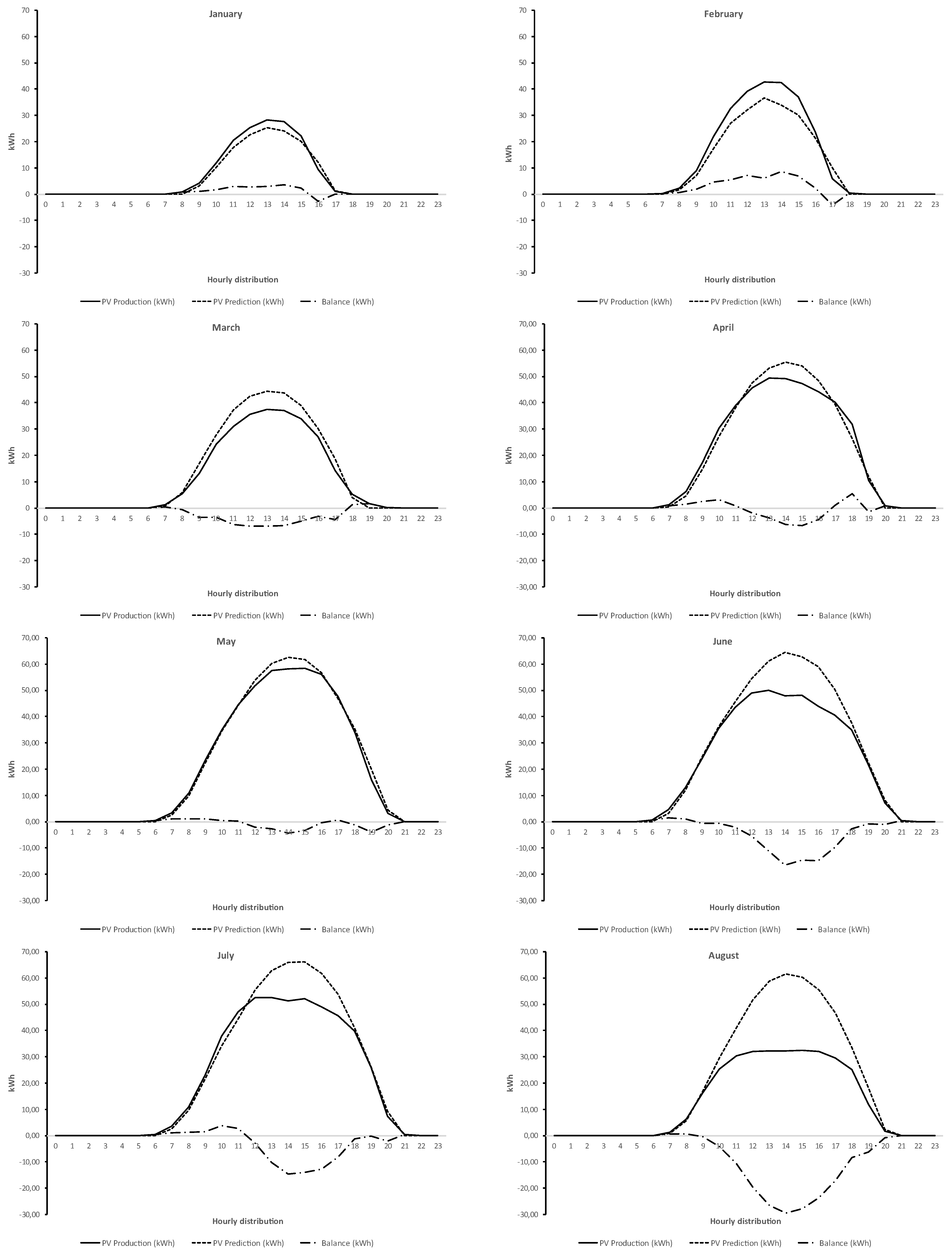
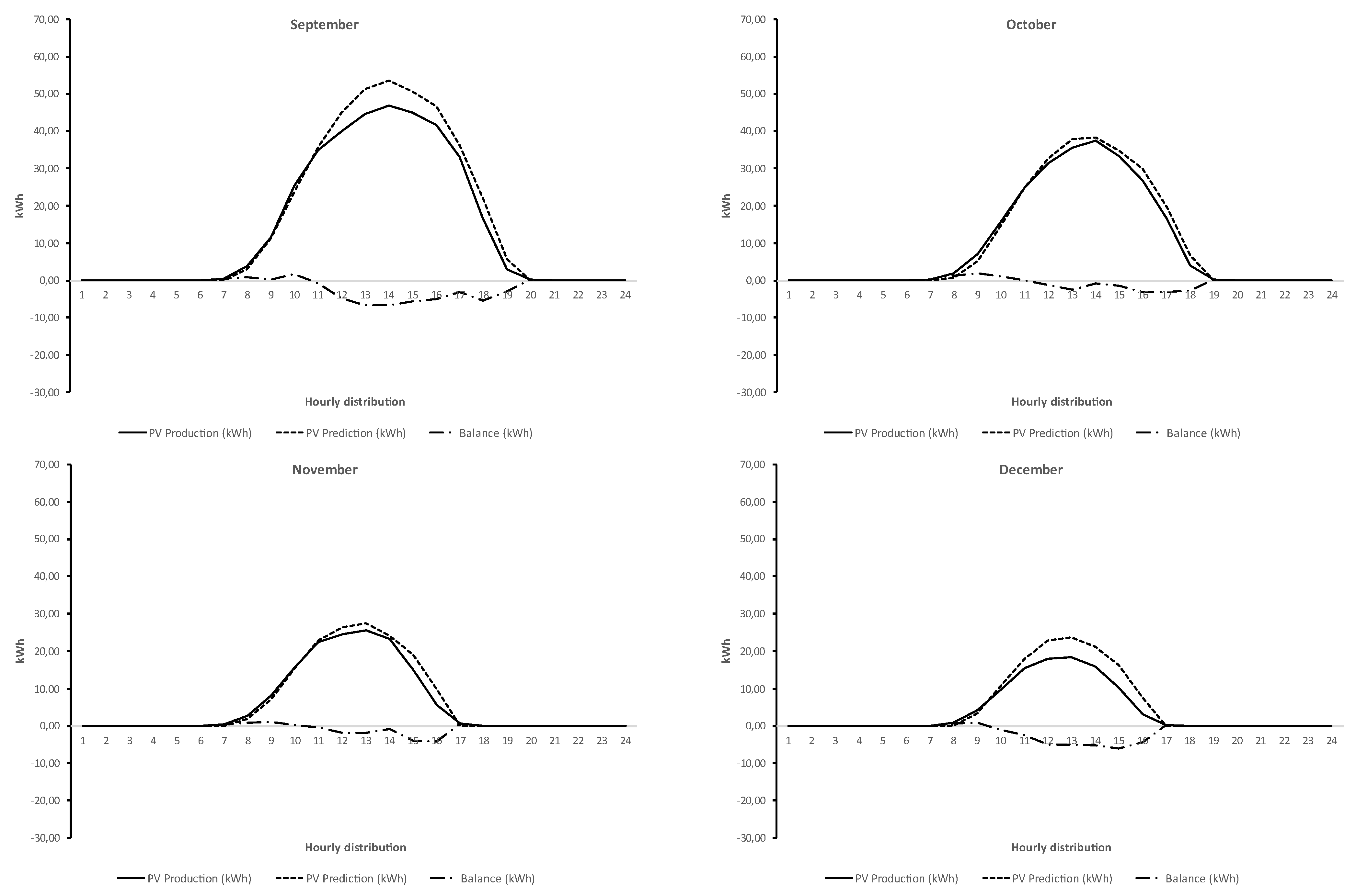
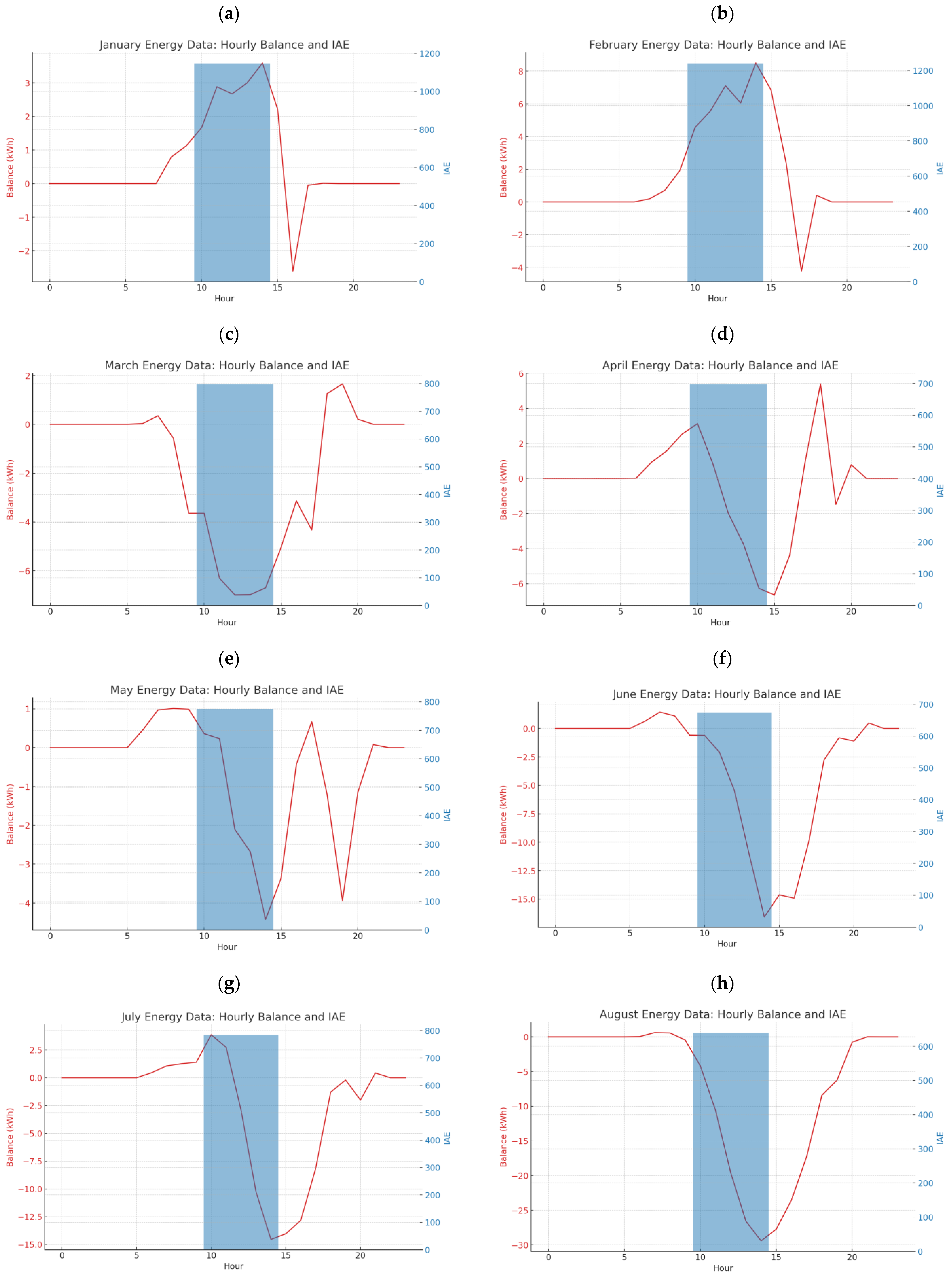
The graphs presented in
Figure 4 show the 12-month production data of the 102.8 kWp photovoltaic system installed at the ESTG campus and the production estimate obtained using the PVGIS (Photovoltaic Geographical Information System) platform (available at
https://joint-research-centre.ec.europa.eu/photovoltaic-geographical-information-system-pvgis_en, accessed on 15 March 2023) based on the data obtained between 2010 and 2020, as well as the balance between these two variables (PV production vs. PV prediction). The analysis of the results shows that when the balance is positive, production is higher than average, and when the balance is negative, it means that the production is lower than the value estimated by prediction. This scenario occurs mainly between March and December, due to the fact the electricity produced by the PV system is not injected into the grid. As expected, this value is higher in the summer months (June, July, and August), because electricity production increases with the solar radiation, and the consumption gradually falls with the end of the school year, reaching a minimum value in August, when the school is almost empty.
When analyzing the results, the integral absolute error (IAE) and standard deviation (SD) are metrics used to quantify errors and variability in data, respectively. The IAE for January is 1146.97, for February it is 1239.58, and for March it is 796.83. These values represent the cumulative absolute differences between consumption and production across each month, indicating that February had the highest imbalance, followed by January, with March being the most balanced month. The standard deviation for January is approximately 12.61, for February it is about 12.83, and for March it is around 13.47. These values measure the variability of the energy balance from the average for each month. A higher standard deviation indicates a larger spread of balance values around the mean. March shows the highest variability, which may be due to the presence of energy production data that slightly offsets the otherwise constant negative balance due to consumption. The IAE for April, May, and June are 696.89, 774.96, and 674.07, respectively. These values indicate that May had the highest total imbalance, suggesting that the energy system faced the largest cumulative shortfall between energy consumption and production during this month. The SD measures the dispersion of the balance values around their mean. The SDs for April, May, and June are approximately 27.70, 32.30, and 27.79, respectively. The higher SD in May corroborates with the IAE findings, suggesting that not only was the imbalance greater in May, but the fluctuations in the balance were also more pronounced compared to April and June. This could imply more variability in either consumption patterns or production output or both during May. Overall, these metrics suggest that the energy system’s performance was most erratic in May, with both higher discrepancies and greater variability in the energy balance. For July, the IAE was calculated at 782.96, indicating the total magnitude of the energy deficit over the month. The SD was 34.87, reflecting the variability in the hourly balance. August showed an improvement with a lower IAE of 638.39 and a smaller SD of 27.69, suggesting a more consistent and closer energy balance between consumption and production. In September, while the IAE increased slightly to 766.03 compared to August, the SD remained relatively similar at 27.83, indicating stability in the balance fluctuations despite the higher total deficit. The reduction in the IAE from July to August implies an overall improvement in the balance, which is possibly due to better energy management or increased production. The consistency in the SD between August and September, despite a higher IAE, might suggest that while the overall deficit increased, the balance did not become more volatile, which could be seen as a positive aspect of energy management for those months. In October, the IAE was 929.20, which reflects the sum of absolute differences between production and consumption. For November, this value slightly increased to 1020.69, suggesting a larger overall imbalance. December showed a reduction in imbalance, with an IAE of 865.09. October had the highest SD at 17.33, indicating that the balance values vary more widely from the mean compared to the other months. November and December had lower SDs of 11.94 and 8.22, respectively, suggesting less fluctuation in the balance values. November had the highest total imbalance, while December had the least. The month of October showed the most variability in its energy balance, whereas December was the most consistent. These results suggest that the energy system’s performance varied, with November being the most challenging month in terms of managing the balance between consumption and production. The results are summarized in
Table 2 and schematically presented in
Figure 5.
Throughout the year, the energy balance data, when considering PV energy production, reveals significant fluctuations in the IAE and SD across different months. The IAE, which measures the cumulative absolute difference between consumption and production, indicates that the energy system experienced the highest imbalance in February and the lowest in March. These variations in IAE could be attributed to changing weather conditions, which directly affect PV energy production, with February perhaps having less sunlight or more cloud cover. The SD reflects the spread of balance values around the mean, with March displaying the highest variability. This suggests that while overall energy production and consumption were more balanced, the hourly fluctuations were significant, possibly due to the erratic availability of solar energy or shifts in consumption patterns. As the year progressed, May exhibited both a high IAE and SD, indicating not only a substantial energy shortfall but also significant variability in energy balance. This could mean that May faced several days with poor solar irradiation or that consumption was particularly high or erratic during this period. The summer months of July and August showed an improvement in the IAE, with August having a lower IAE and SD, suggesting a better-managed energy balance, potentially due to longer daylight hours enhancing PV energy production. In the latter part of the year, November presented the greatest challenge with the highest IAE, reflecting a substantial energy deficit. However, the SD was lower in November and December compared to October, indicating less variability despite the higher deficits. This could be due to shorter daylight hours leading to reduced PV production, coupled with possibly consistent consumption patterns. Overall, the data suggest a correlation between the balance of PV energy production and consumption with seasonal changes. The variability and deficits in energy production could have consequences such as increased reliance on non-renewable energy sources or the need for energy conservation measures during periods of low PV output. The energy management strategies must therefore account for these fluctuations to enhance the reliability of PV energy throughout the year.
In comparison to other regions, the performance of our installed photovoltaic system aligns with global trends of increased efficiency and productivity in solar energy generation. Specifically, when juxtaposing our results with systems in similar climatic zones, we observe that the energy production potential in our study is consistent with the higher end of PV output reported in Mediterranean climates. For instance, studies on PV systems in regions like Southern Spain and Italy show comparable seasonal productivity patterns, particularly with peak production in the summer months. Nevertheless, our case stands out in its ability to maintain a relatively high level of production efficiency during the winter months, surpassing the average yields of similar latitude installations by a noticeable margin. This suggests that the specific technological choices and management strategies implemented in our system may offer valuable insights for optimizing photovoltaic energy production in educational institutions, which could be beneficial when considering the design and operation of PV systems in these environments worldwide.
The high IAE values observed indicate a significant discrepancy between experiment and prediction. This large error could be a result of several factors. Firstly, the method of prediction used may not be well-suited to the complexity or nature of the data. If the model is too simple or does not capture all the influential variables, it could lead to inaccurate predictions and thus a high IAE. Secondly, the quality of the data used for training and testing the model could be a contributing factor. Data that are noisy, contain outliers, or are non-representative of the system can lead to poor model performance. Thirdly, the parameters and settings of the model could be suboptimal. This might include the learning rate, the number of layers in a neural network, or the selection of features used for prediction. It is also possible that the large IAE could be due to a fundamental change in the system that occurred after the model was trained, which the model could not anticipate. From this, and analyzing all possibilities, it is entirely possible that the high IAE could be attributed to the use of real-measured data that are subject to natural variability, such as daily sunlight hours, cloud cover, and other environmental factors. These factors can introduce a significant amount of unpredictability into the system being modeled, especially in contexts such as renewable energy production where solar and wind power outputs can fluctuate dramatically due to weather conditions.
If the predictive model was developed under the assumption of certain stable conditions or without accounting for the full range of natural variability, this could lead to a mismatch between predicted and actual values, hence a high IAE. For instance, if the model for predicting solar power output was trained on data from a period with consistent weather patterns, it might not perform well when faced with the more variable conditions that naturally occur over different seasons or weather events. To address this, in a future approach, the model can be enhanced by incorporating weather-related variables directly into the model if they are not already included. Machine learning models can be equipped to handle complex, non-linear relationships and interactions between variables, which might capture the impact of environmental factors more accurately; utilize more sophisticated time series analysis techniques that can account for seasonal trends, cyclical patterns, and other temporal dynamics; implement a dynamic modeling approach that updates predictions based on real-time data inputs, allow the model to adjust to current conditions; consider stochastic modeling techniques that can factor in the inherent randomness of certain inputs and offer a range of possible outputs with associated probabilities; or even increase the granularity of the data, which might involve using hourly measurements instead of daily averages, to capture fluctuations more accurately. In this way, by refining the predictive model to take into account the stochastic nature of environmental factors, the accuracy of predictions shall improve, and the IAE shall decrease accordingly.
Justifying the high IAE found with environmental variability can indeed be supported by looking at the relationship between the IAE and SD from the data obtained. The SD reflects the variability or spread of the individual errors around the mean error, which, in the context of environmental data, can be indicative of natural fluctuations. In the results, months like April, May, June, July, and September exhibit both a relatively lower IAE and a higher SD compared to other months like January and February, which have a higher IAE but a lower SD. This suggests that even though the predictive errors (IAEs) for the former set of months are lower, the variability of these errors is greater, which could be indicative of the impact of environmental factors such as changes in weather. For instance, the higher SD in the summer months (April through July) could be due to the greater variability in weather conditions, like cloud cover and the number of sunlight hours, which are more pronounced during these months and can affect solar energy production predictions. Despite this variability, the IAE is relatively low, which might suggest that the prediction model is somewhat robust to these changes, but not entirely accurate. Conversely, the winter months (November and December) show a lower SD and a higher IAE. This could imply that while the variability due to environmental factors is less pronounced (possibly due to consistently poorer weather conditions), the prediction errors are higher, which might suggest other factors at play, such as a model that does not account well for seasonal changes.
4.2. Analysis of the Evolution of Production, Consumption, and Balance in an Annual Time Horizon
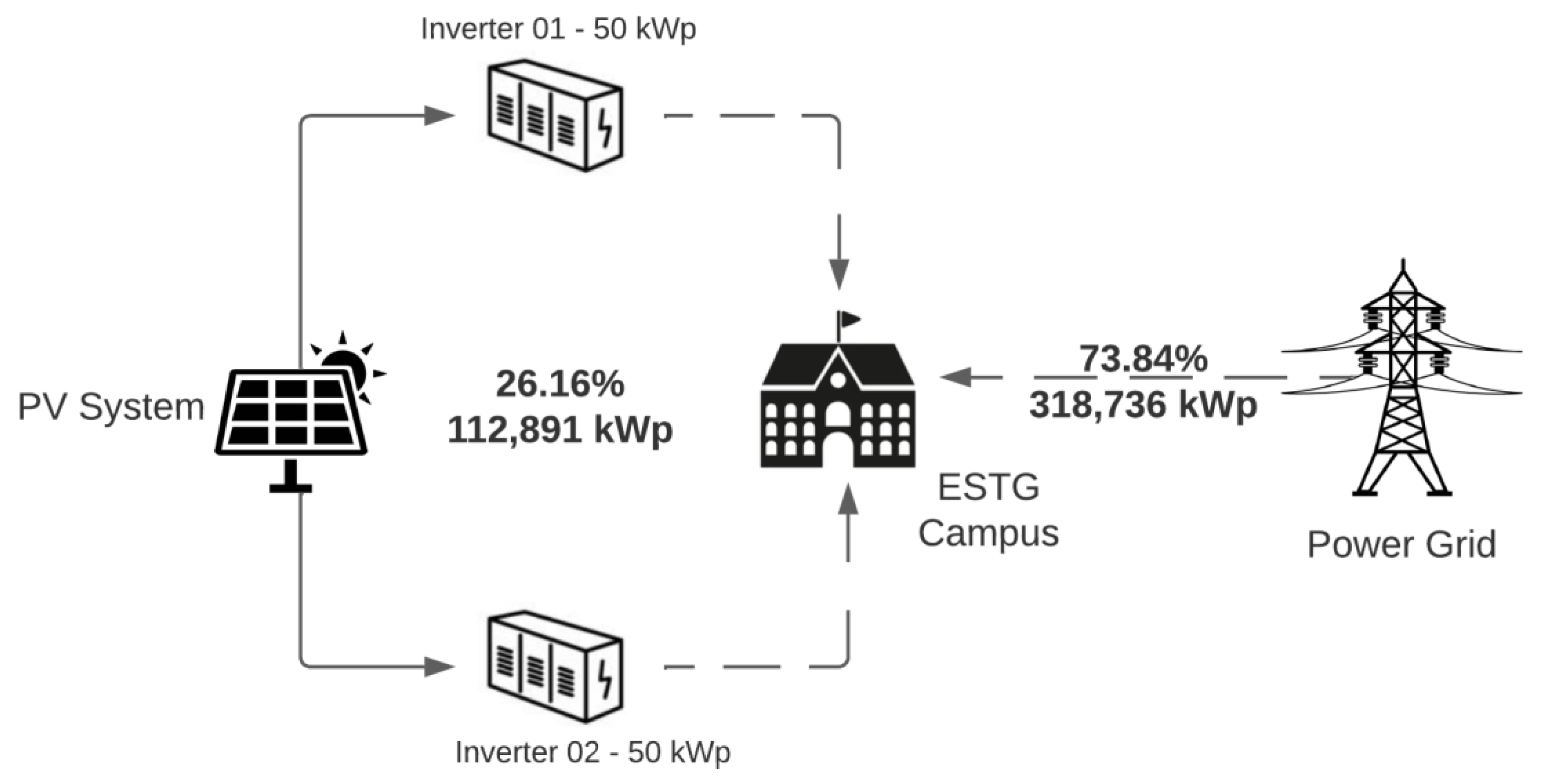
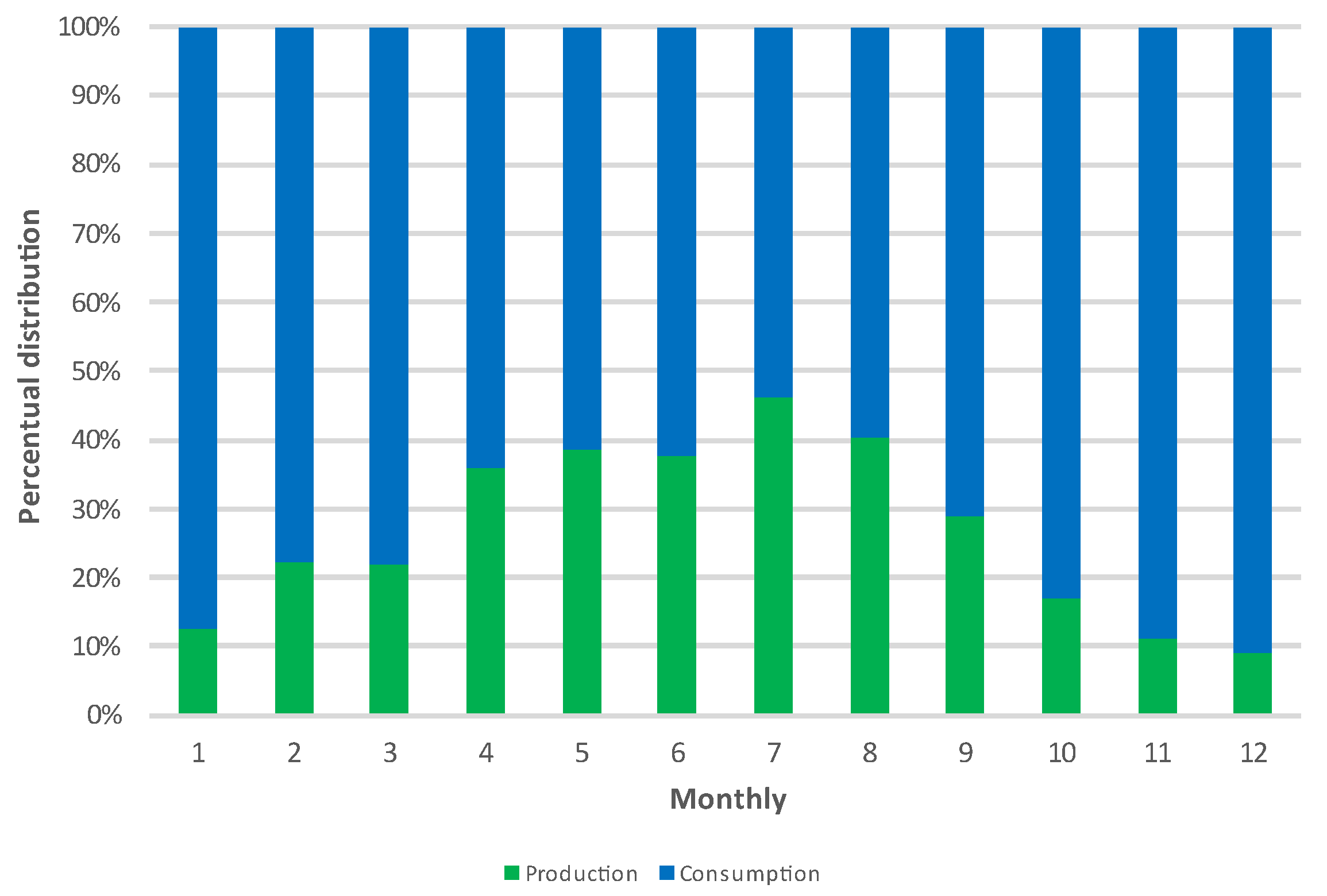
The installation of renewable energy systems to produce electricity for self-consumption, as is the case of the situation under analysis in this article, presupposes that the photovoltaic system installed can offset at least a significant part of consumption since this is the only possible way to amortize the investment made by reducing electricity costs. From a purely economic analysis of the situation, it seems that the total estimated PV energy produced corresponds to 26.1% of the campus consumption on average (
Figure 6). In a first analysis, this value seems to be relatively reduced due to several factors: there is high energy consumption on the campus during the non-production period, at night, and in some specific periods of the year, energy consumption is lower than the energy production, so the potential production is not at its maximum because the installed system is designed without grid injection, and, based on this, the system’s inverter cuts and blocks energy production according to the consumption profile.
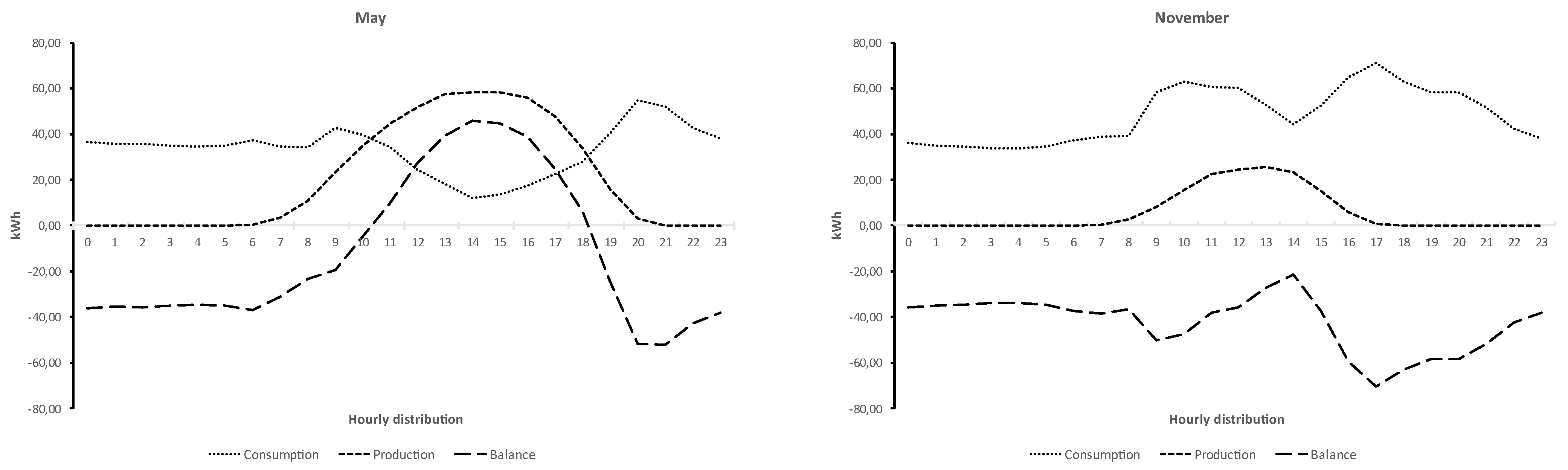
The graphs in
Figure 7 show how the installed photovoltaic system works in a so-called “typical month”, which is associated with the highest and the lowest annual energy production. By considering the summer and winter solstices and the building’s consumption periods, it was decided to analyze the months of May and November as examples of a “typical month” for summer and winter, respectively. By analyzing the monthly hourly average energy production for the two graphs, it can be observed that in May, the production corresponds to 38.49% of the total energy consumed, while in November, the production only reaches 11.01%. If the same analysis is carried out by considering the average period between sunrise and sunset, from 6 a.m. to 9 p.m., in May, the energy production corresponds to 49.69% of the total energy consumed, i.e., there are significant differences in the system’s performance depending on the period of analysis.
This discrepancy in the system’s performance between both periods of the year influences the produced energy usage profile, which is derived from the model imposed by the legal framework laid down in the contract of the funded project. According to the current application model for the project that financed the installed PV system, there is no possibility to inject the produced energy into the grid. In other words, if there is no consumption on the campus, there will be no energy production, so there is no way of using the surplus energy to repay the original investment. As the periods of photovoltaic energy production coincide with the building’s peak use periods, it is also certain that, even in the winter months, there will be maximum use of the energy produced.
Based on this, the question that needs to be answered is the following: what should be done when the site has excess power generation that cannot be injected into the grid, and how should different amounts of energy produced throughout the year be efficiently managed? A straightforward alternative to the problem would be to install a battery system to accumulate surplus energy, allowing it to be used in periods outside the range of PV energy production. However, there is not yet a complete consensus on the effectiveness of this system and, above all, on the investment required, given the campus energy needs. To guarantee greater storage capacities and high reliability, the cost of a battery system can be expensive and cost as much as the photovoltaic system as a whole (panels, inverters, and power optimizers). Additionally, batteries are hard to maintain (in a sealed lead-acid deep cycle battery, for instance, the water levels have to be checked periodically, and the terminals kept clean); the useful life of a battery will depend on the type of battery to be used and its discharge capacity, which is usually low, and, due to environmental issues, they are not recommended because components are hard to be recycled.
Another solution to the problem would be to take advantage of the accurate forecast of the PV energy production schedules and make users aware of the need to adjust major energy consumers to these periods, especially those that are routine as they are associated with normal operating activities, such as the cafeteria, canteen, or laboratory services. Where possible, this change can be supplemented with an automatic load management and consumption monitoring system, changing behaviors, and reorganizing tasks so that, as far as possible, they are carried out in intervals during the period of PV energy production. In this way, consumption is carried out using the PV energy produced, rather than the energy supplied by the power grid, thereby effectively helping to reduce energy costs.
Last but not least, energy communities and/or collective self-consumption are a viable way of improving the performance of a photovoltaic system. This shared vision of the energy issue allows the overproduction to be shared with other neighborhood installations that are operating during the PV energy production period and are out of phase with the peak consumption of the campus where the photovoltaic system is located. For example, sports facilities (pavilions and swimming pools) near the school campus have high energy usage on the weekends when there is practically no school activity, and hotels in the vicinity consume energy mainly in the morning period and from 5 pm onwards. Additionally, if there is still room in the PV production period, the generated energy can be used to heat domestic hot water using electric resistance, preheat water for other types of use, or use air conditioning systems, which should operate only at times when there is an excess of energy production. These possibilities allow the maximization of the use of the photovoltaic energy production system, relying on a good control and monitoring system to manage energy usage in real-time.
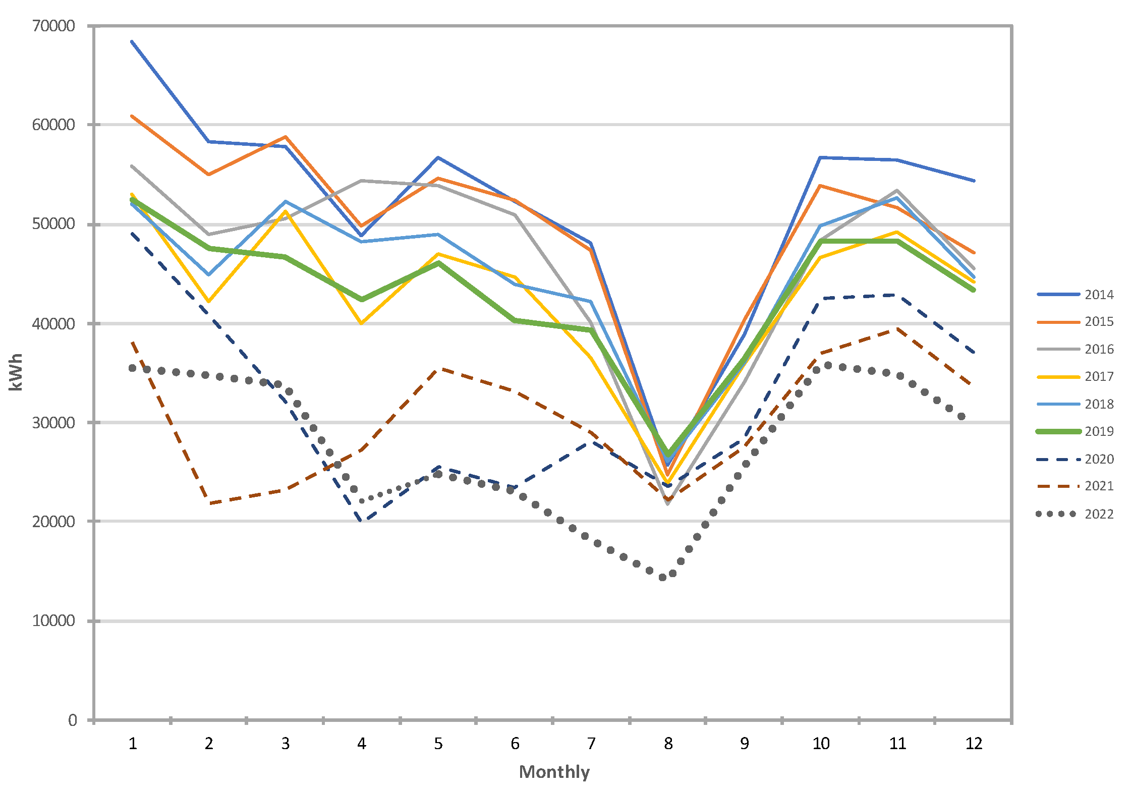
4.3. Distribution of Monthly Consumption Data from 2014 to 2022
The graphs presented in
Figure 8 show the consumption per month of the grid energy and the production of the photovoltaic system that will be spent on the campus since the system does not allow injection into the grid. The total consumption of the campus would be the grid energy consumption plus the photovoltaic production. Daily photovoltaic production rarely exceeds energy grid consumption, and the grid energy consumption is never zero because there are periods during the night when there is no sun and therefore PV production does not occur. It is also possible to observe that consumption drops considerably on the weekend, as expected, and the same happens with PV production because it is a system without grid injection and forces the inverters to cut production.
Figure 8 also shows the history of monthly consumption from 2014 to 2022; 2020 and 2021 were atypical years due to the global COVID-19 pandemic.
As mentioned before, photovoltaic production is already reflected in this figure for 2022, which means that the reduction in the energy consumption visible in this graph is due to the funded project that was implemented. The main energy efficiency measures, besides PV system installation, were the following: replacement of the existing lighting with LED technology, replacement of the window frames and shading devices, addition of thermal insulation to the roof and the buildings’ facades, replacement of two natural gas boilers with two low-condensation, high-efficiency natural gas boilers, and installation of a rooftop to improve summer thermal comfort.
This graph depicts the monthly consumption data of an entity from 2014 to 2022 measured in kWh. Multiple lines represent different years, allowing for a comparative analysis over time. It is observable that consumption trends follow a similar pattern annually, with two noticeable peaks around the 3rd and 9th months, which likely correspond to periods of higher activity or operational demands, possibly due to seasonal variations or academic calendars if related to an educational institution. In 2020 and 2021, there is a distinctive drop in consumption, potentially reflecting reduced operations due to the global COVID-19 pandemic. The data for 2022 present a visible decrease in consumption compared to previous years (except 2020 and 2021), possibly indicating the implementation of energy-saving measures or the integration of alternative energy sources like photovoltaic systems. The dashed line representing 2022 suggests either projected data or ongoing data collection for this period. It is also worth noting the overall variability in consumption, indicating a dynamic energy usage pattern subject to various influencing factors.


