Article

Whole Life Cycle Cost Analysis of Transmission Lines Using the Economic Life Interval Method

1
State Grid Sichuan Economic Research Institute, Chengdu 610095, China
2
State Grid Sichuan Information & Communication Company, Chengdu 610041, China
3
College of Electrical Engineering, Sichuan University, Chengdu 610065, China
*
Author to whom correspondence should be addressed.
Energies 2023, 16(23), 7804; https://doi.org/10.3390/en16237804
Submission received: 7 November 2023 / Revised: 22 November 2023 / Accepted: 24 November 2023 / Published: 27 November 2023
(This article belongs to the Special Issue Modern Power System Stability and Optimal Operating)

Abstract

:
With the large-scale construction and commissioning of transmission lines over the past two decades, the grid is facing a large-scale centralized decommissioning of transmission lines. The transmission line’s economic life is crucial to rationalizing its construction and reducing the grid’s development costs. Based on the minimum economic life calculation principle, the static and dynamic transmission line economic life calculation model is established, considering the whole life cycle for transmission line cost. The improved gray GM (1,1) model is applied to forecast cost data during the economic life assessment of transmission lines with fewer samples. Considering the cost uncertainty in life-cycle costing, the interval cost model based on the coefficient of variation wave amplitude is proposed to determine the economic life intervals under different guarantees by using the normal distribution probability density function, which reduces the influence of cost fluctuations on the economic life calculation error. The economic life analysis of a 500 kV transmission line is used as a case study to verify the model’s accuracy and effectiveness. The method shows the economic life intervals under different guarantee degrees based on the most probable economic life determination, which provides theoretical support for calculating the economic life elasticity of transmission lines.

1. Introduction

With China’s economy rapidly developing, investment in the power grid is also increasing [1]. Operating, maintaining, and upgrading the grid is becoming increasingly complex [2]. Power transmission lines possess unique characteristics as power equipment. A transmission line is a type of power equipment that possesses unique characteristics [3]. The investment cost of the power transmission line exceeds 50% of the electrical project’s total cost. Replacing the line without proper analysis would result in economic losses for the power grid company. Assessing the line’s economic viability requires an effective balance of economic, reliability, and safety factors. Currently, transmission line projects are analyzed using technical methods that do not adequately consider economic costs [4]. As the power system reform deepens, the traditional rough management mode is no longer adequate for lean management requirements. To optimize management strategies and asset utilization, it is necessary to evaluate the economic lifespan of transmission line projects. This will provide theoretical support for technical reform and investment, making it vital for the related companies.
Due to the extensive construction and operation of transmission lines over the past two decades, the grid is facing a large-scale, concentrated decommissioning of transmission lines. Large-scale, centralized decommissioning of transmission lines has implications for both grid companies and users. On the one hand, power grid companies must arrange significant funds, manpower, and materials to renew and reconstruct lines within a tight schedule. On the other hand, this effort poses potential risks to users’ safe and reliable electricity use [5]. Meanwhile, uncertainty about the timing of economic decommissioning affects the operational decisions of grid companies. Therefore, it is necessary and practical to consider the uncertainty of the costs incurred by transmission lines to perform the life assessment of transmission lines, rationalize the arrangement of investment in the renewal and construction of transmission lines, and ensure the supply of electricity [6].
According to the concept of life cycle management, this work analyzes the costs associated with investment, operation, maintenance, and failure of transmission line projects based on previous works. At the same time, considering the influence of uncertainty factors, the technical evaluation method and the theory of interval method are utilized to establish the transmission line project’s economic life interval measurement model. The main contributions of this work are as follows:
(1)
Static and dynamic transmission line economic life calculation models are developed, considering the life cycle cost of transmission lines.
(2)
Cost data are forecasted even with limited samples based on the improved GM (1,1) model.
The rest of this paper is organized as follows: Section 2 analyzes the state of the art; Section 3 introduces the economic life interval method for transmission lines; Section 4 illustrates the case study; Section 5 discusses the results of this work; and Section 6 concludes this paper and suggests future work.

2. State of the Art

There have been studies on the economic lifespan of power equipment, both domestically and internationally, analyzing the life cycle cost in practice. Hu et al. [7] proposed a grid asset economic efficiency evaluation model that considers safety and efficiency factors and applies them to transformers. Zhang et al. [8] studied the operation and economic evaluation of the integrated energy system with hydrogen storage equipment in the electricity and carbon markets. It also calculated the life-cycle investment benefit of a community-integrated energy system with hydrogen storage equipment. By extending the life cycle approach, Chen and Ou [9] proposed a new approach to estimate carbon emissions and costs in energy transmission and distribution. It also applied the approach to a 220 kV substation in Fujian Province and showed its life cycle’s economic and carbon costs. Zhang et al. [10] used a cost–benefit model to calculate and compare fuel and electric vehicles’ economic costs and carbon emissions over their whole life cycle. They analyzed the future trend of the emission reduction benefits of electric vehicles using an improved gray forecast model. Regarding practical analysis, the whole life cycle is more often applied to the carbon market and the evaluation of assets. On the other hand, these studies are focused on life cycle cost modeling. Li et al. [11] built a power transformer life cycle calculation model that considered vital factors in all sections of the life cycle and researched the economic life evaluation method to obtain the least total cost in the life cycle. Wang and Fu [12] utilized the lambert-w function to find the exact solution for the total annual allocated cost and economic life of a power transformer. Chen et al. [13] developed an economic life forecast model for transformers based on the maximum annual average net profit criterion and various economic factors. Wang et al. [14] established an optimized equipment life estimation model using an improved genetic algorithm. However, most of the current economic life cost models focus on transformers, and there are fewer studies on the economic life of lines. However, as transmission lines are installed in complex and changing outdoor environments for a long time, the uncertainty of damage faced by lines occurs from time to time. Thus, determining the economic life interval of the line under uncertain conditions is a practical guideline for the rational design of the decommissioning and renewal construction plans of transmission lines.
Transmission line projects face complex environments and long line construction and operation times. The analysis of economic life needs to consider the uncertainty of operating costs, maintenance costs, and failure costs. It also reflects the time value of money. The calculation of the economic life is based on the operating costs for each year of the line’s life cycle. Therefore, there is a need to forecast the line operating cost. The gray model (GM) and the autoregressive integrated moving average (ARIMA) model are now widely used. Yang et al. [15] used an improved GM to forecast oil consumption trends. Zhao and Shi [16] forecasted oil and gas operating costs during production reduction periods with improved GM. Liu et al. [17] predicted coal mining costs with an improved GM. The GM is mainly used for cost forecasting in various domains. Fekri et al. [18] used an ARIMA model to improve the accuracy of the prediction data to train an energy prediction model for the power grid. Zhao et al. [19] used the ARIMA model to forecast residential construction costs. ARIMA forecasting is not limited to costs but can also be used for output forecasting. Each forecasting method is adapted to different scenarios. This work conducts a study to compare and contrast the GM, which is found to be more applicable to line operating cost forecasting. The improved GM model is used to predict the operating cost trend of transmission lines, considering the increasing deterioration rate of transmission lines, and to provide data support for their economic life analysis.

3. Methodology

3.1. Theoretical Analysis of Transmission Lines’ Economic Life Modeling

Replacing transmission lines does not enhance the production capacity of the electric utility, nor does it generate additional revenues. As a result, transmission line asset renewals do not result in new cash inflows for electric utilities. Consequently, it is advisable to only factor in the costs associated with the program’s entire lifespan when making decisions regarding transmission line renewal.

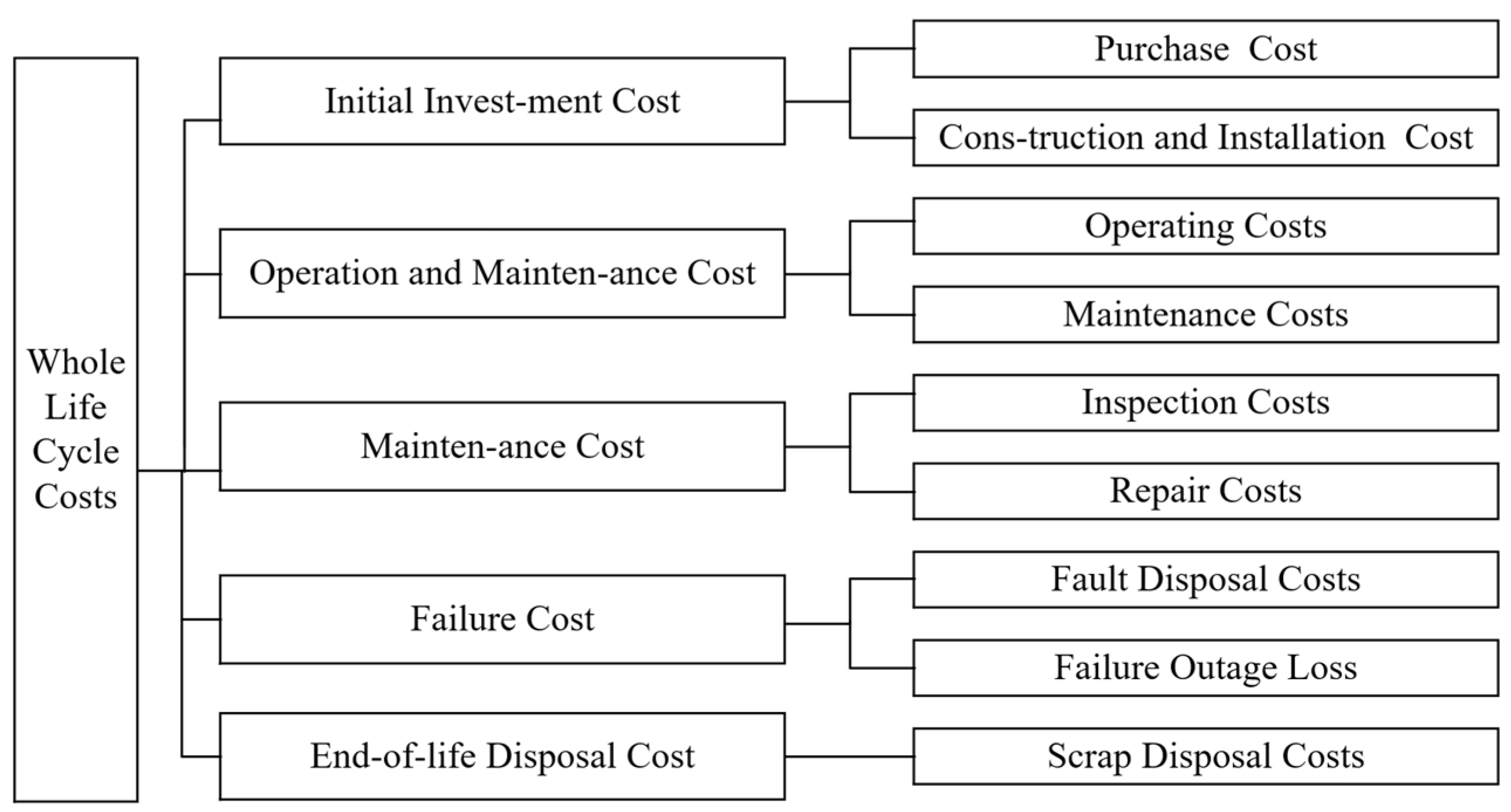
3.1.1. Transmission Line Life Cycle Costs

The design of a transmission line’s whole life cycle is intended to manage and optimize the systems, processes, and costs of all phases of a project. This includes preplanning, design, purchase of equipment, construction, maintenance, and recovery. The goal is to maximize economic, social, and environmental benefits through the integration of design, construction, and operations to ensure that the project’s functions, life, and costs are synchronized with each other throughout the life of the project. By integrating the design, construction, and operation of the transmission line, the project will maximize economic, social, and environmental benefits while also achieving functional harmonization, lifetime harmonization, and cost balancing throughout the life cycle of the transmission line project. Whole life cycle costs are costs incurred throughout the service period of a project, from investment and construction to end-of-life disposal, specifically including the initial investment cost, operation and maintenance cost, maintenance cost, failure cost, and end-of-life disposal cost. Revenue from the salvage value of assets is used to offset the disposal cost. The composition of the whole life cycle cost is shown in Figure 1. Operation and maintenance costs, maintenance costs, and fault costs are incurred during the use of transmission lines, which are closely related to the operation status and belong to the operation costs.

3.1.2. The Economic Lifetime of Transmission Lines

Economic life is the period during which a piece of equipment remains in use and meets the economic demands of the system. The economic life of a transmission line corresponds to the service life when the total annual cost of the entire transmission line process is at its lowest. This is determined by considering the entire life cycle of the transmission line. Economic life refers to the economically viable period of a transmission line, during which only life cycle costs are considered during renewal. Therefore, in this paper, the lowest total annual cost is used as an indicator to determine the economic life of transmission lines.
Transmission lines are characterized by significant initial investment, long in-service times, and high exposure to the natural environment. As transmission lines remain in service for longer, the annual equalization of initial investment and end-of-life disposal costs gradually decreases. However, with the extension of line service time, the degree of line deterioration accelerates significantly, the adverse impact of external natural conditions is increasingly significant, the incidence of failure increases, and the cost of operation and maintenance, maintenance, and fault disposal rises rapidly. As the service life increases, the lower value of investment and end-of-life disposal costs will be offset by an increasing value of operating costs. The upfront investment in transmission lines is significant, with investment and end-of-life disposal costs dominating the upfront cost components. Transmission line operation and maintenance costs, maintenance costs, and fault disposal costs rapidly increase in the later stages of transmission line operation, so these costs dominate. In cost changes, the average annual total cost decreases and then increases, showing a “U” shape. There must be a point in the project’s natural life cycle where the average annual total cost is the lowest during the transmission line’s economic life.
Determining the economic life of a transmission line is a judgment as to whether the operating costs incurred by the transmission line in the next year as the line’s time in service increases will result in a lower or unchanged total equivalent annual cost. Suppose the total equivalent annual cost decreases or remains the same as the transmission line remains in service. In that case, the transmission line is economically viable and has not yet reached the economic life of the transmission line. If the equivalent annual cost is increased, the transmission line is no longer economically viable for continued use, and decommissioning must be considered. Therefore, obtaining the total equivalent annual cost of a transmission line and its variability becomes the key to determining the economic life of a transmission line.

3.2. Transmission Line Economic Life Model

Transmission line economic life algorithms can be divided into two categories: static economic life and dynamic economic life. The dynamic calculation method determines the minimum useful life of the total annual cost, considering the time value of money. The static calculation methods do not consider the time value of money and are classified as cost-averaging and uniformly low-degradation numerical methods. Therefore, static calculations are primarily analyzed using the cost-averaging method.

3.2.1. Static Transmission Line Economic Life Model

The static transmission line economic life model consists mainly of the average annual shared cost of the initial investment and the average annual operating cost [7]. Without considering the condition of time and the value of money, the model for calculating the economic life using the annual equivalent total cost method can be expressed as Equation (1).
A C L = P S L L + 1 L j = 1 L ( O C j + M C j + F C j )
where A C L is the total equivalent annual cost of the transmission line at L years of service. P is the initial investment cost of the line. S L is the net salvage value of equipment discarded at the end of the L year. j is the year of use for the line, and j [ 1 , L ] . L is the number of years the line has been in service. O C j , M C j , and F C j are the transmission line operation and maintenance costs, maintenance costs, and fault costs, respectively, for the j-th year of the L -year service life. The sum of the three makes up the annual operating cost of the line.

3.2.2. Dynamic Transmission Line Economic Life Model

Transmission lines are in service for long periods after being put into operation, and the time value of money dramatically impacts the economic life of a transmission line. When considering the time value of money, the economic life model of a transmission line calculated using the annual equivalent total cost method can be expressed in Equation (2).
A C L = [ P S L × ( P / F , i , L ) + j = 1 L ( O C j + M C j + F C j ) × ( P / F , i , j ) ] ( A / P , i , L )
where i is a composite discount rate. ( P / F , i , L ) = 1 / ( 1 + i ) L , ( P / F , i , j ) = 1 / ( 1 + i ) j are the discount factors. ( A / P , i , L ) = 1 / ( 1 + i ) L / ( 1 / ( 1 + i ) L 1 ) .
The operating costs incurred by the project each year are based on the current year’s prices, so the impact of the producer price index (PPI) on purchasing power needs to be considered. The discount rate i c is corrected using the PPI f . The corrected composite discount rate is calculated as in Equation (3).
i = i c f 1 + f
where i c is the social discount rate taken as 8%. f is the rate change in the PPI, taken as 5%.

3.2.3. Updated Decision-Making Model

After the transmission line annual equivalent total cost model is established, the problem of determining the economic life of the transmission line is converted to solving for the in-service time that minimizes the A C L model with L as the independent variable [11].
N = L | min A C L
where a i j compares the importance of element i and element j .

3.3. Improved GM (1,1) Cost Forecasting Model

The modeling process of the gray forecast model GM (1,1) is to model the irregular raw data after accumulating them and obtaining the generating series with a high degree of regularity. Then, the data obtained from the generated model are calculated to bring the forecasted values of the original data. In the measurement of economic lifetimes, except for the simplified numerical method and GM, which can be calculated when the initial investment and a few years of operating data are known, most of the remaining models require the operating costs of each year of the line’s life cycle to perform the calculations. GM is characterized by its ease of use, poor information, small sample sizes, and being particularly well suited to trend changes in data. Operating costs tend to increase significantly with the years of service, consistent with the characteristics of the object to be served by the GM. We applied an improved GM (1,1) cost forecast model to overcome the fixed weight problem in traditional GM. Improved GM uses the automatic optimization and weighting method to select the weight values that give the model the highest forecast accuracy, thereby improving the accuracy of the forecast. Adjusting the baseline data values accounts for the current accelerated decay rate of the transmission line. The improved GM (1,1) forecast process enhances the impact of recent data at the forecast point and provides data support for economic life analysis.

3.4. Cost Range Calculation Based on Variation Coefficients

This section is divided by subheadings. It provides a concise and precise description of the experimental results, their interpretation, and the practical conclusions that can be drawn.
As transmission lines are operated with different work contents, fault probability, and scale each year, it is not easy to accurately estimate yearly costs. To make the calculation results more practically instructive, the forecasted annual operating costs of transmission lines are extended to annual operating interval costs. Based on the clarification of the most probable economic life of transmission lines, the economic life interval of transmission lines is determined to provide flexibility in scheduling transmission line renewal decisions. Annual operating costs fluctuate on an overall incremental basis, and the calculation of average annual operating costs can further flatten the volatility of the data to ensure that the data fluctuations are regular and continue to change smoothly. Therefore, a transmission line economic life interval calculation method is proposed using the forecasted fixed value as the most probable annual operating cost value, using the previous numerical background value coefficient of variation as the amplitude reference, and using the amplitude to calculate the cost interval data. Operating cost fluctuations for each year are calculated in Equations (5) and (6).
γ k = η k 1 , d × y ¯ k 1 , d × y ˜ ( k )
η k 1 , d = i = k 1 d k 1 ( y ˜ ( i ) y ¯ k 1 , d ) 2 d / x ¯ k 1 , d
where γ k is the fluctuation of the operating cost range in year k . η k 1 , d is the variation coefficient of operating costs in year k 1 for the forward d years. y ¯ k 1 , d is the average of the annual operating costs in year k 1 for the forward d years. y ˜ ( k ) is the kth-year operating cost.
The range of operating cost variations can be determined by the cost fluctuation γ k as [ y ˜ ( k ) γ k , y ˜ ( k ) + γ k ] . y ˜ ( k ) is considered the most likely operating cost and has the highest probability of occurrence. Using y ˜ ( k ) γ k and y ˜ ( k ) + γ k as the main range bound for the data distribution has the lowest probability of occurrence. The likelihood of incurring operating costs fluctuates around the most probable costs in decreasing directions. This is similar to the normal distribution probability density function, so it is assumed that the probability of the operating cost distribution satisfies the normal distribution. By the 3 σ laws of probability theory, P { μ 3 σ < X < μ 3 σ } = 99.74 % . This probability means that 99.74% of the data fall within μ ± 3 σ . Therefore, the probability density function of the normal distribution of operating costs is constructed in terms of μ = y ˜ ( k ) and σ = γ k / 3 , as shown in Figure 2.
Due to the imperfect forecastability of costs, operating costs have different probabilities of occurring within cost intervals. For this, a method of calculating cost intervals with varying degrees of guarantee is proposed. Using μ as the cost likelihood value and μ as the symmetric axis, extend the value t on either side and the area encircled by the x-axis as the guarantee level. The degree of guarantee ζ is calculated as in Equation (7).
η k 1 , d = i = k 1 d k 1 ( y ˜ ( i ) y ¯ k 1 , d ) 2 d / y ¯ k 1 , d
From Figure 2, it can be seen that when μ = y ˜ ( k ) and t = 0 , the degree of guarantee ζ = 0 is the lowest, and the economic life interval degenerates to a fixed value of economic life as the most probable value. When t = 3 σ , the guarantee ζ = 99.74 is the highest, and the calculated economic life is the upper and lower limits of the value of the economic life. Equation (7) and Figure 2 can be used to determine the cost ranges for different guarantees, thus determining the economic life of different guarantees.
The steps for calculating the economic life of a transmission line when considering the guarantee degree are as follows:
Determine the degree of guarantee value ζ .
Obtain the probability corresponding to the probability μ f ( t ) d t by querying the standard normal distribution table.
Calculate the normal distribution probability μ t f ( t ) d t , by reversing Equation (7), i.e., μ t f ( t ) d t = μ f ( t ) d t ζ / 2 .
Calculate the guarantee ζ boundary μ ± t . The μ t corresponding to the probability μ t f ( t ) d t is obtained by querying the standard normal distribution table, which is a lower bound on the cost under the degree of guarantee ζ . Similarly, calculate the guaranteed upper bound μ + t .
Calculate the static and dynamic economic life at each year’s upper and lower operating cost bounds, and determine the economic life interval at the guarantee ζ .

4. Results Analysis

4.1. Data

This work discusses a 500 kV overhead transmission line in Sichuan and assumes that during the operation of the transmission line, the climatic conditions will follow the pattern of the past 10 years and there will be no extreme disasters such as blizzards, major earthquakes, floods, etc. It calculates the economic life of the line using the economic life model under an improved GM (1,1) average annual operating cost forecast. The initial investment for the 500 kV transmission line was CNY 37.53 billion. The social discount rate i c = 8 % . The composite discount rate i = 2.86 % . Based on data ranging from 2005 to 2015, annual operating cost projections are subsequences of the commencement of service on the line.
A screening process was performed to ensure forecast accuracy. Operation and maintenance costs (OC), maintenance costs (MC), fault disposal costs (FC), operating costs, and average annual operating costs are the selected forecasting factors, and their variations are graphically displayed in Figure 3. The smoothness of the curves depicting the yearly maintenance expenses and FC displayed is inadequate, and there is no assurance regarding the accuracy of the forecasts. OC, FC, and MC multi-indicator data forecast the cumulative tendency to cause error accumulation problems. FC and MC are significant components of annual operating costs. To maximize the accuracy of the data, the average annual operating cost is selected as the forecast in this work.

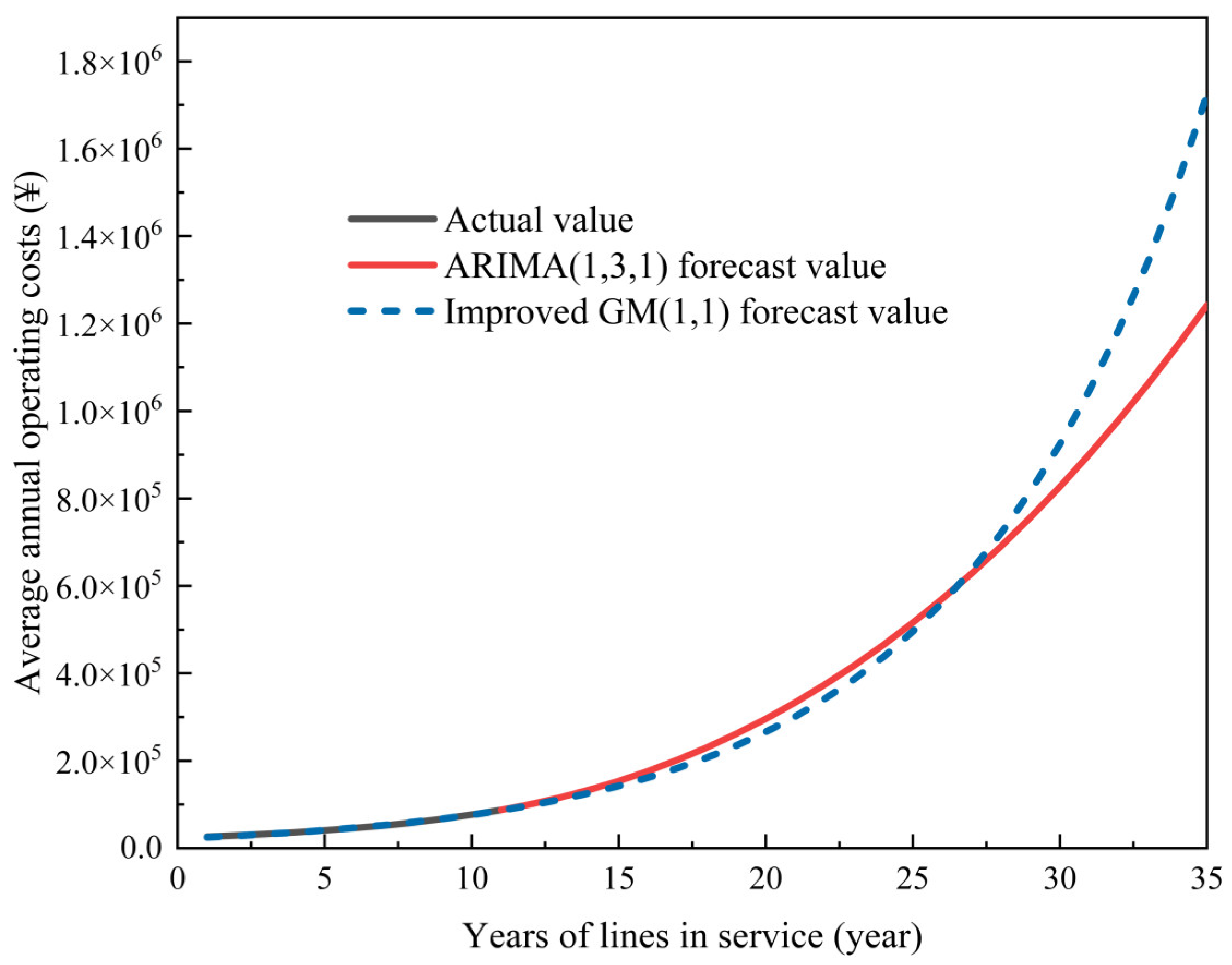
4.2. Improved GM (1,1) Cost Forecasting Results

This work is run in a MATLAB environment and on an AMD Ryzen 7 5800 H with Radeon Graphics @3.20 GHz. The improved GM (1,1) was used to forecast average annual operating costs and make a rank-order judgment on the average annual operating cost series. The maximum and minimum values of the original series rank ratio are within the required range of rank ratios. Therefore, it can be forecasted using GM (1,1). The data and errors for forecasting the average annual operating cost of the line are shown in Table 1. Regarding data accuracy, the relative error of the forecast model is 0.0173; the average grade deviation is 0.00177. The model forecasts results with high accuracy.
The model GM (1,1) coefficients and forecasted values were obtained as follows:
y ^ ( 1 ) ( k ) = 18.65 + 2.4964 e 0.1246 ( k 1 )
In this work, the comparison is made with the improved GM through the ARIMA model. The optimal model of ARIMA is obtained as ARIMA (1, 3, 1) by using the average annual operating cost data from 2005 to 2015. The model coefficients and forecasted values were obtained based on the forecast results.
y t = 0.01564 0.49465 × ( 1 1.08 3 ) y t ( 1 1.08 3 ) ε t 1
The forecasted values of the two methods are obtained, as shown in Figure 4. The ARIMA (1, 3, 1) model forecasts mainly from the 12th year onwards, and the relative error of the method cannot be calculated here. However, the improved GM (1,1) forecasts from the first year and calculates the relative error between the actual and forecasted values. Figure 4 shows that the difference between the two methods’ forecasts increases after the 27th year. Later, when calculating the economic life of the transmission line, the ARIMA (1, 3, 1) model could not provide a feasible solution. Therefore, the GM (1,1) average annual operating cost forecast results are used in this paper.
The general agreement between the model-forecasted trend and the actual temperature trend is shown in Figure 4. This work analyzes the historical average annual operating costs using only the historical average annual operating costs. It does not consider the impact of other factors on costs comprehensively. However, the model’s forecast effect has a slight inaccuracy with the actual value, indicating that the model is feasible.

4.3. Transmission Line Economic Life Interval Results

Using the average annual operating cost data for the forecasted completion, the total operating cost for the forecasted year is calculated by Equation (10).
y ~ t = y t ( k ) × ( k ) y t ( k 1 ) × ( k 1 )
To compare the economic life interval under different guarantee degrees, different guarantee degrees are selected to calculate the economic life interval. When ζ = 0 , the economic life interval decreases to a constant economic life. And d = 5 . When ζ = 0.5 , checking the standard normal distribution table gives μ f ( t ) d t = 0.5 . By consulting the standard normal distribution table, the probability μ t f ( t ) d t = 0.25 corresponds to t = 0.675 σ . Using μ ± t as the upper and lower cost limits for a guarantee of 0.5, the kth-year operating costs for different guarantees are shown in Table 2.
Substituting the above-calculated operating cost intervals under different guarantee degrees into the static and dynamic economic life Equations (1) and (2), the economic life intervals under different guarantee degrees can be obtained, and the results of the calculations are shown in Figure 5 and Figure 6.
As can be seen from Figure 5 and Figure 6, when the guarantee degree is 0, using the static calculation method, the economic life of the 500 kV transmission line is 24 years, and the average annual cost is CNY 1,117,956. When the dynamic calculation method is used and the time value of money is considered, the economic life of the transmission line is 24 years, and the average annual cost is CNY 1,746,679. When the guarantee degree is 0.5, using the static calculation method, the economic life of the transmission line is 24 years, and the average interval cost is [1,115,718, 1,120,195]. When the dynamic calculation method is used and the time value of money is considered, the economic life of the transmission line is 24 years, and the average cost of the interval is [1,744,863, 1,748,494]. When the guarantee degree is 1, using the static calculation method, the economic life interval of the transmission line is [24, 25], and the average interval cost is [1,115,718, 1,120,195]. When the dynamic calculation method is used and the time value of money is considered, the economic life of the transmission line is 24 years, and the average cost of the interval is [1,738,610, 1,754,747]. The economic life interval model is based on a fixed economic life as the most probable economic life of the line. It is extended to both sides of the fixed economic life in the form of reduced probability, corresponding to the actual situation and improving the theoretical guidance.

5. Discussion

To verify the rationality of the economic life interval model, the results of the economic life interval calculations (Figure 4) and (Figure 5) are listed in Table 3. As can be seen from Table 3, the economic life ratings are all within the economic life interval, which contains the economic life ratings. When ζ = 0 , the economic life interval degenerates to a constant economic life value. This validates the correctness of the economic life interval model in this paper. In practice, the decommissioning life of transmission lines is mostly about 25 years, which also further validates the rationality of the proposed economic life interval model. The economic life interval model is based on a fixed economic life as the most probable economic life of the line, which is extended to both sides of the fixed economic life in the form of reduced probability. This work utilizes the life cycle economic life calculation principle to establish a comprehensive model for calculating the economic life interval of transmission lines, both statically and dynamically. By optimizing for the minimum equivalent annual total cost, this model achieves a more accurate evaluation of transmission line economic life. Additionally, an improved GM (1,1) model with fewer samples is introduced to enhance the accuracy of cost data prediction during the evaluation process. This work is contextualized and enhanced with theoretical guidance.

6. Conclusions

Based on the transmission line economic life interval calculation model, the simulation results are as follows:
  • The improved GM (1,1) forecasting model can be better applied to line operating cost forecasting.
  • The proposed economic life interval calculation model effectively considers the uncertainty of costs incurred during operation.
  • Expanding economic life from a fixed value to an interval reduces the impact of cost fluctuations on calculating economic life, enhancing practical guidance.
In future research, it would be beneficial to delve deeper into the impact of the environment. Presently, predictions are based solely on generalized historical data, despite the fact that transmission lines are exposed to the outdoor environment for prolonged periods, leaving them susceptible to unpredictable damage. By examining further data, future studies can improve the comprehensiveness and reliability of their findings. Categorizing external environmental factors can also provide a more detailed analysis of transmission line lifespan, which can aid in making more precise decisions regarding renewal.

Author Contributions

Conceptualization, W.Z. (Wenhui Zeng); methodology, J.F.; validation, W.Z. (Wentao Zhang); software, Y.L.; visualization, B.Z.; formal analysis, R.H.; investigation, X.X.; resources, J.L. All authors have read and agreed to the published version of the manuscript.

Funding

This work was supported by the Science and Technology Project of the State Grid Sichuan Electric Power Company (521996220002).

Data Availability Statement

Data are contained within the article.

Conflicts of Interest

The authors declare no conflict of interest.

References

  1. Zhao, F.; Xue, L.; Zhu, J.; Chen, D.; Fang, J.; Wu, J. A novel investment strategy for renewable-dominated power distribution networks. Front. Energy Res. 2023, 10, 968944. [Google Scholar]
  2. Li, Z.; Xu, Y.; Wang, P.; Xiao, G. Coordinated preparation and recovery of a post-disaster Multi-energy distribution system considering thermal inertia and diverse uncertainties. Appl. Energy 2023, 336, 120736. [Google Scholar] [CrossRef]
  3. dos Santos, C.H.F.; Abdali, M.H.; Martins, D.; Alexandre, C.B.A. Geometrical motion planning for cable-climbing robots applied to distribution power lines inspection. Int. J. Syst. Sci. 2021, 52, 1646–1663. [Google Scholar] [CrossRef]
  4. Huang, W.; Zhang, N.; Yang, J.; Wang, Y.; Kang, C. Optimal Configuration Planning of Multi-Energy Systems Considering Distributed Renewable Energy. IEEE Trans. Smart Grid 2019, 10, 1452–1464. [Google Scholar] [CrossRef]
  5. Li, Z.; Xu, Y.; Wang, P.; Xiao, G. Restoration of Multi-Energy Distribution Systems with Joint District Network Reconfiguration by A Distributed Stochastic Programming Approach. IEEE Trans. Smart Grid 2023. early access. [Google Scholar] [CrossRef]
  6. Khalyasmaa, A.I.; Uteuliyev, B.A.; Tselebrovskii, Y.V. Methodology for Analysing the Technical State and Residual Life of Overhead Transmission Lines. IEEE Trans. Power Deliv. 2021, 36, 2730–2739. [Google Scholar] [CrossRef]
  7. Xu, N.; Chen, M.; Liu, Z.; Nie, J.; Wang, Y.; Song, S. The Security Effectiveness Assessment of Power Grid Assets Based on Life Cycle. In Proceedings of the 4th International Conference on Advances in Energy Resources and Environment Engineering, Chengdu, China, 7–9 December 2018; IOP Publishing Ltd.: Bristol, UK, 2019; p. 062031. [Google Scholar]
  8. Zhang, Y.; Zhao, Q.; Ao, J.; Wang, Z.; Wang, Y. Full life-cycle economic evaluation of integrated energy system with hydrogen storage equipment. E3S Web Conf. 2022, 338, 01018. [Google Scholar] [CrossRef]
  9. Chen, X.; Ou, Y. Carbon emission accounting for power transmission and transformation equipment: An extended life cycle approach. Energy Rep. 2023, 10, 1369–1378. [Google Scholar] [CrossRef]
  10. Zang, L.; Xiao, B.; Ma, J.; Liu, Y.; Tian, P.; Zhang, L. Research on the cost effectiveness of carbon emission reduction in the full life cycle of electric vehicles based on grey prediction. MATEC Web Conf. 2022, 355, 02031. [Google Scholar] [CrossRef]
  11. Li, N.; Wang, X.; Zhu, Z.; Wang, Y.; Han, J.; Xu, R. The Research on the LCC Modelling and Economic Life Evaluation of Power Transformers. IOP Conf. Ser. Mater. Sci. Eng. 2019, 486, 012030. [Google Scholar] [CrossRef]
  12. Wang, J.; Fu, L. Power transformer life analysis based on Lambert W function. J. Phys. Conf. Ser. 2022, 2221, 012009. [Google Scholar] [CrossRef]
  13. Hu, B.; Chen, Q.; Rao, W.; Qiao, J. Economic Life Prediction of Transformer Based on Repairing Profit and Decommissioning Profit. J. Phys. Conf. Ser. 2019, 1314, 012113. [Google Scholar] [CrossRef]
  14. Wang, Y.; Wang, S. Life prediction of power Internet of Things equipment based on improved genetic algorithm. In Proceedings of the International Conference on Cloud Computing, Internet of Things, and Computer Applications (CICA 2022), Luoyang, China, 28 July 2022; Powell, W., Tolba, A., Eds.; SPIE: Bellingham, WA, USA, 2022; p. 81. [Google Scholar]
  15. Yang, Y.; Chen, Y.; Shi, J.; Liu, M.; Li, C.; Li, L. An improved grey neural network forecasting method based on genetic algorithm for oil consumption of China. J. Renew. Sustain. Energy 2016, 8, 024104. [Google Scholar] [CrossRef]
  16. Yue, Z.; Diyi, S. Oil-gas Cost in The Declining Period Predicting Model Based on Self-adaptive GM(1, 1,λ). In Proceedings of the 2021 6th International Conference on Intelligent Computing and Signal Processing (ICSP), Xi’an, China, 9–11 April 2021; IEEE: Piscataway, NJ, USA, 2021; pp. 69–72. [Google Scholar]
  17. Liu, D.; Li, G.; Chanda, E.K.; Hu, N.; Ma, Z. An improved GM (1.1) model with background value optimization and Fourier-series residual error correction and its application in cost forecasting of coal mine. Gospod. Surowcami Miner. Miner. Resour. Manag. 2019, 35, 75–98. [Google Scholar]
  18. Fekri, M.N.; Ghosh, A.M.; Grolinger, K. Generating Energy Data for Machine Learning with Recurrent Generative Adversarial Networks. Energies 2019, 13, 130. [Google Scholar] [CrossRef]
  19. Awad, A.S.A.; EL-Fouly, T.H.M.; Salama, M.M.A. Optimal ESS Allocation and Load Shedding for Improving Distribution System Reliability. IEEE Trans. Smart Grid 2014, 5, 2339–2349. [Google Scholar] [CrossRef]
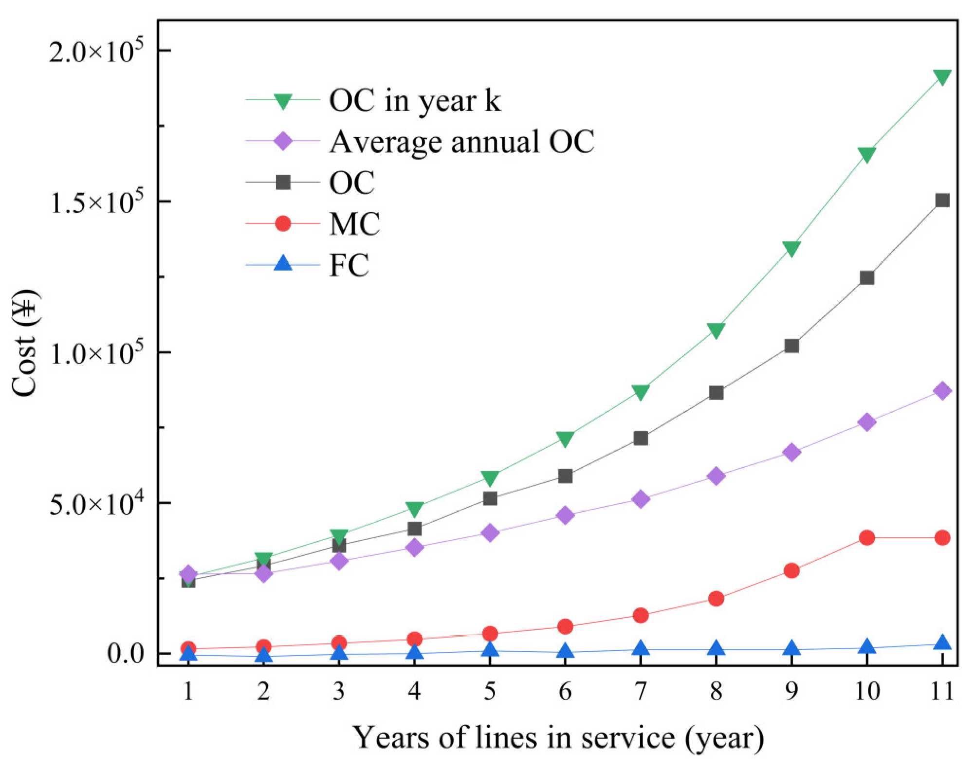
Figure 1. Whole-life cost components.
Energies 16 07804 g001
Figure 2. Cost range and occurrence probability.
Energies 16 07804 g002
Figure 3. Line cost trend.
Energies 16 07804 g003
Figure 4. Line cost trend.
Energies 16 07804 g004
Figure 5. Static average annual total cost and economic life range of the line.
Energies 16 07804 g005
Figure 6. Dynamic average annual total cost and economic life range of the line.
Energies 16 07804 g006
Table 1. The average annual operating cost forecast data and error.
YearActual Value (CNY)Forecast Value (CNY)Relative Standard Deviation
126,60024,963.940.061506
229,40028,275.130.038261
332,70032,025.500.020627
436,50036,273.320.006210
540,90041,084.570.004513
646,00046,533.970.011608
751,90052,706.170.015533
858,90059,697.050.013532
967,20067,615.190.006178
1077,00076,583.580.005408
1187,40086,741.520.007534
Table 2. The annual operating costs of transmission line intervals at different assurance levels.
YearVariation Coefficient η Fluctuation γ ζ = 0 ζ = 0.5 ζ = 0.1
120.335.5120.13[18.89, 21.37][14.62, 25.63]
130.336.4623.83[22.37, 25.28][17.36, 30.29]
140.327.5828.15[26.44, 29.85][20.57, 35.72]
150.328.8733.18[31.18, 35.17][24.31, 42.04]
160.3210.3739.03[36.70, 41.36][28.66, 49.40]
170.3112.1145.84[43.11, 48.56][33.73, 57.94]
180.3114.1253.74[50.56, 56.92][39.62, 67.86]
190.3116.4562.92[59.22, 66.62][46.47, 79.37]
200.3119.1573.56[69.25, 77.87][54.41, 92.70]
210.3122.2685.89[80.88, 90.90][63.62, 108.15]
220.3025.86100.16[94.34, 105.98][74.30, 126.02]
230.3030.02116.68[109.92, 123.43][86.66, 146.70]
240.3034.82135.78[127.94, 143.61][100.96, 170.59]
250.3040.35157.84[148.77, 166.92][117.49, 198.20
260.3046.73183.33[172.82, 193.84][136.60, 230.02]
270.3054.08212.74[200.58, 224.91][158.66, 266.83]
280.3062.55246.67[232.60, 260.75][184.13, 309.22]
290.2972.29285.79[269.53, 302.06][213.50, 358.09]
300.2983.51330.87[312.08, 349.66][247.37, 414.38]
310.2996.40382.80[361.11, 404.49][286.39, 479.20]
320.29111.23442.57[417.55, 467.60][331.34, 553.80]
330.29128.27511.36[482.50, 540.23][383.09, 639.64]
340.29147.85590.49[557.23, 623.76][442.64, 738.35]
350.29170.34681.48[643.15, 719.81][511.14, 851.82]
Table 3. Different guarantees of calculation results.
Static Economic LifeDynamic Economic Life
Guarantee degree ζ = 0 ζ = 0.5 ζ = 1 ζ = 0 ζ = 0.5 ζ = 1
Annual costCNY 1,117,956[1,115,718, 1,120,195][1,115,718, 1,120,195]CNY 1,746,679[1,744,863, 1,748,494][1,738,610, 1,754,747]
Economic life2424[24, 25]242424
Disclaimer/Publisher’s Note: The statements, opinions and data contained in all publications are solely those of the individual author(s) and contributor(s) and not of MDPI and/or the editor(s). MDPI and/or the editor(s) disclaim responsibility for any injury to people or property resulting from any ideas, methods, instructions or products referred to in the content.

