Study on Market-Based Trading Strategies for Biomass Power Generation Participation in Microgrid Systems

Abstract

The Chinese government places significant importance on biomass energy due to its renewable and environmentally friendly attributes. However, the high cost of power generation poses a considerable hurdle to its development. This study aims to address the challenges facing the profitability and sustainable development of biomass power generation after the gradual withdrawal of the Chinese government by proposing a day-ahead real-time market-based trading strategy. It is prompted by the incentives offered by the Chinese government for the ongoing power market reform. This strategy is developed for a microgrid system that integrates biomass power generation with other renewable energy sources. The principles followed by the microgrid system include self-generation and consumption, electricity surplus sales, and electricity shortfall procurement. During the day-ahead stage, peak and valley tariffs are decided by the microgrid operator to exert influence on the incentives of capacity providers in accordance with the load trends, while in the intraday stage, the supply-demand imbalance is resolved by the stored electricity. In the trading process, marginal production and marginal pricing are specified to ensure the minimum trading volume and price for capacity traders, ensuring their profitability. It is demonstrated in this study that the trading strategy presented is more effective than conventional fixed-price trading in making biomass power generation profitable and sustainable, even after the Chinese government subsidy is phased out. Moreover, the other participant in the microgrid system can boost their earnings when compared to generating power individually for trading.

1. Introduction

With the introduction of peak carbon and carbon neutral targets, the focus of electricity system reform has shifted from promoting the monopoly segment of the grid to the development and consumption of large-scale renewable energy sources [1]. In this context, it is essential to accelerate the popularization of wind power (WD), photovoltaic (PV), and other types of renewable energy, and to promote the construction of a novel power system [2].

At present, most of the research on biomass power generation has focused on power generation models and how to enhance efficiency. Additionally, the research has paid attention to the current state of development and policy-related concerns [3]. In References [4,5,6], the current state of the global biomass power generation industry is analyzed. Additionally, a discussion is conducted about the future trends of biomass power generation and its sustainability. In Reference [7], it is demonstrated that both options of the biomass gasification cogeneration (BGCHP) system contribute significantly to energy conservation and create environmental benefits. However, the paper is limited to examining the characteristics of BGCHP power generation, with its profitability ignored. In light of this, the power generation model is constructed in this study.

In terms of energy trading, previous studies have focused mainly on examining the trading methods from the perspective of stakeholders. In References [8,9,10], it is explored how cogeneration in biomass power generation enhances unit thermal efficiency and boosts revenues. However, trading remains based on government-subsidized prices. According to References [11,12], decentralized power sources and loads should establish their contracted power levels in the day-ahead power market and engage in real-time power market trading. This requires the use of an integrated demand response two-tier optimization model that takes into account both the maximum advantages for the energy suppliers and the minimum energy costs for the consumers. Nevertheless, these studies overlook the generation of biomass power for commercial benefits. It is thus essential to investigate its engagement in market-oriented transactions for its improved sustainability. In References [13,14], the all-renewable multi-energy complementary system is optimized through “wall-separated electricity sales” to reduce the total annual cost. However, capacity unit revenues were overlooked. In References [15,16], an investigation is conducted into waste-to-energy incineration, which demonstrates that cogeneration enhances unit thermal efficiency and thus boosts revenues. However, it overlooks the advantages of participating in market-based trading. In Reference [17], the overall integrated benefits of microgrids and generation-side revenue are effectively enhanced through coordinated planning. However, no attention is paid to the utilization of biomass and waste resources as well as the benefit analysis of generating electricity for market-based trading.

Based on the above analysis, it is necessary to cope with the policy demand of developing and consuming large-scale renewable energy resources in the context of power market reform, to construct a novel power system, and to enhance the sustainable development of biomass energy and its profitability. In order to construct a microgrid system of renewable energy, a day-ahead real-time market-based trading strategy is proposed in this study. In the day-ahead stage, with the volatility of WD and PV power generation taken into account, electrolysis (EL) tanks were set up to ensure that the power is fully utilized. Additionally, marginal prices and marginal outputs were established for BGCHP and waste incineration cogeneration (WICHP), which ensures a minimum level of power output for cogeneration and enhances its overall profitability. By establishing marginal tariffs for WD and PV energy, their minimum selling price is ensured. In the intraday stage, the energy in storage (ES) is used to address the supply-demand imbalance. Finally, the proposed strategy is verified through simulation, and the results of trading as obtained under this strategy are quantitatively analyzed.

2. Transaction Participants and Protective Regulations

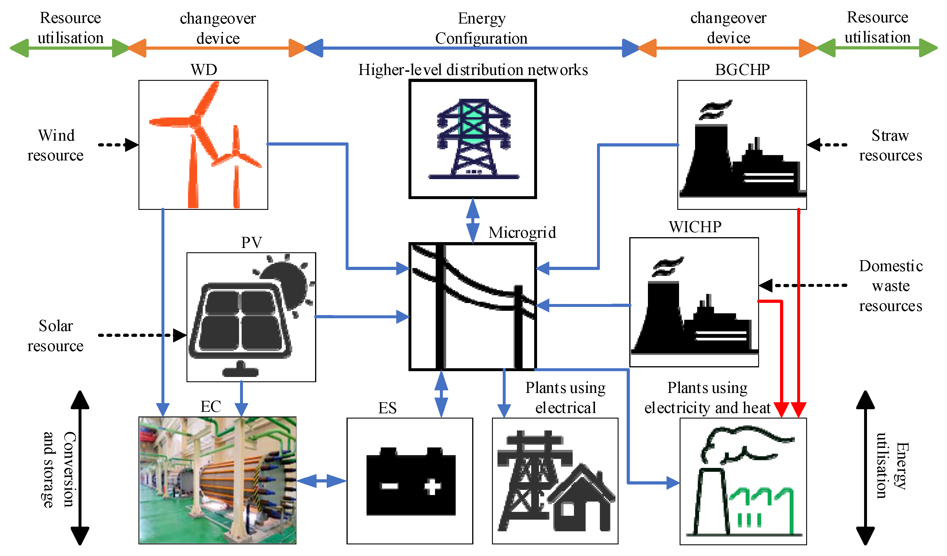
2.1. Modeling of Microgrid Systems

In this paper, a microgrid system is constructed, as shown in Figure 1. This system operates on the principle of “self-generation and self-consumption, electricity surplus sales, and electricity shortfall purchase”. The capacity units within the system consist of multiple renewable energy sources, with an EL incorporated for the regulation and utilization of electricity.

The microgrid consists mainly of a capacity provider, an operator, a load aggregator, an upper-level source network, and an ES device controlled by the operator.

Among them, the capacity provider is comprised of BGCHP, WICHP, WD, and PVs. It is intended to generate both electricity and heat.

The operator is responsible for the acquisition, storage, and selling of electricity and thermal energy. Its main function is to provide a fair, secure, and legally effective trading platform for energy trading.

Load aggregators are comprised of multiple energy users within the region who engage in market-based trading. Their role is to coordinate and consolidate loads, and to ensure a more cost-effective and stable energy supply by enabling their participation in market-based transactions as a unified load entity. Load aggregators are nonprofit organizations.

Electricity storage plays a regulatory role when the imbalance between supply and demand occurs. Electricity storage is operated by the operator as a nonprofit dispatch unit.

The upper-level source grid is a higher-tier grid compared to the microgrid described in this paper. Its primary role is to provide a source of backup energy supply source for the system loads.

2.2. A Model of Quoting Strategies for Market-Based Trading Entities

2.2.1. Modelling of Cogeneration Units and Their Bidding Strategies

The cogeneration units in this paper are BGCHP and WICHP. BGCHP is designed to harness straw resources in rural areas as fuel for the production of electricity and industrial steam [7]. WICHP aims to utilize municipal waste resources in urban areas as fuel for generating electricity and industrial steam [16]. Their power generation has a rated capacity of 30 MW, and their steam supply pressure is set at 1.2 MPa. Their general models are represented by Equation (1).

$$\{\begin{array}{l}24.98\le P{E}_{\mathrm{x},t}^{\mathrm{RQ}}\le 30\\ P{H}_{\mathrm{x},t}^{\mathrm{RQ}}=\left({\eta }_{\mathrm{x},h}/{\eta }_{\mathrm{x},e}\right)P{E}_{\mathrm{x},t}^{\mathrm{RQ}}\\ R{L}_{\mathrm{x},t}=\left(3.6P{E}_{\mathrm{x},t}^{\mathrm{RQ}}\right)/\left({\eta }_{\mathrm{x},e}\cdot {\sigma }_{\mathrm{x}}^{\mathrm{RZ}}\right)\end{array}$$

(1)

where ${\eta }_{\mathrm{x},e}$ and ${\eta }_{\mathrm{x},h}$ represent the electrical and thermal efficiencies of the unit, respectively; ${\sigma }_{\mathrm{x}}^{\mathrm{RZ}}$ indicates the average calorific value of the fuel in MJ/kg; $R{L}_{\mathrm{x},t}$ denotes the fuel consumption in kg; and $P{E}_{\mathrm{x},t}^{\mathrm{RQ}}$ and $P{H}_{\mathrm{x},t}^{\mathrm{RQ}}$ denote the electrical and thermal power in MW in the $t$-time period, respectively. The minimum output of their electrical power is 24.98 MW. The minimum power guarantees are detailed in the section on marginal tariffs.

The marginal tariff generates energy in response to the changes in system loads, sells the electricity generated competitively, and supplies heat at the peak and bottom prices for profit. Marginal tariffs and marginal production are intended to ensure profitability, and the marginal cost of marginal power is the lowest selling price for competitive bidding, as described in Section 2.3.

2.2.2. Modelling Bidding Strategies for WD and PV Power

WD is a green power generation unit that relies on wind energy for electricity generation, whose rated capacity is 50 MW. PVs is a green power generation unit designed to convert solar energy into electricity, with a rated capacity of 30 MW. Their output, denoted as $P{E}_{\mathrm{xp},t}^{\mathrm{RQ}}$, is divided into three parts: $P{E}_{\mathrm{xp},t}^{\mathrm{FH}}$ for load consumption, $P{E}_{\mathrm{xp},t}^{\mathrm{RW}}$ for sinks to the grid, and $P{E}_{\mathrm{xp},t}^{\mathrm{P}2\mathrm{G}}$ for use by the EL. The power acquired by the EL is denoted as $P{E}_{\mathrm{P}2\mathrm{G},t}^{\mathrm{RQ}}$, and it is expressed as Equation (2).

$$\{\begin{array}{l}P{E}_{\mathrm{xp},t}^{\mathrm{RQ}}=P{E}_{\mathrm{xp},t}^{\mathrm{FH}}+P{E}_{\mathrm{xp},t}^{\mathrm{RW}}+P{E}_{\mathrm{xp},t}^{\mathrm{P}2\mathrm{G}}\\ P{E}_{\mathrm{P}2\mathrm{G},t}^{\mathrm{RQ}}=P{E}_{\mathrm{FDp},t}^{\mathrm{P}2\mathrm{G}}+P{E}_{\mathrm{GFp},t}^{\mathrm{P}2\mathrm{G}}\end{array}$$

(2)

The electricity supplied by WD and PVs to the system loads is set for competitive sales on marginal tariffs in accordance with the national standards of 6.43 cents/kWh and 5.88 cents/kWh. These prices are the minimum bid values.

2.2.3. Model for the Operator’s Bidding Strategy

The operator procures capacity from capacity providers based on the system load profile. Through the forecast day-ahead load (represented by the red curve in the figure), the operator determines an average load reference line (represented by the green dotted line in the figure) through calculation, as illustrated in Figure 2 below. Then, considering the distribution of load between peak and valley periods, an intervention tariff is introduced, with different rates set for the peak and valley periods above and below the daily average reference line. Through the estimation of load changes, this intervention pricing is designed to influence capacity providers in terms of capacity incentives.

Based on the peak and valley segments, the size of the difference from the reference line is used as the basis for calibrating the size of the intervention price. Reference line 1 represents the lower boundary value for the calibrated peak hour, while Reference line 2 signifies the upper boundary value for the calibrated valley period. The loads during the hours above reference line 1 represent peak-hour loads, those below reference line 2 are valley-hour loads, and the loads falling between reference lines 1 and 2 are usual-hour loads.

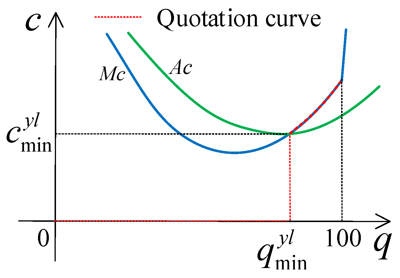
2.3. Marginal Price and Guaranteed Output

The power producers submit quoted prices and quantities at prices higher than their short-term marginal costs. The relationship between marginal cost and marginal output, denoted as blue curve $Mc$, signifies the minimum cost of production at a given marginal output level [18,19], as illustrated in Figure 3.

The point at which the curve of average production cost, represented as green curve $Ac$, intersects with that of the marginal production cost is represented by $q_{\min }^{yl}$, indicating the minimum output level required for profitability. To the right of this intersection point lies the optimal range of economic production, as indicated by the red curve in the figure above. In this context, the fixed cost is equivalent to the construction expenses, while the variable cost includes both O&M (operation and maintenance) expenses and fuel costs. The power level at which the curve of the average production cost intersects with that of the marginal production cost is 83.27% of the rated power [18,19]. Thus, the minimum output is determined to be 24.98 MW for both BGCHP and WICHP.

In this way, Equation [20], which describes the relationship between the marginal cost and marginal output for BGCHP and WICHP, can be approximated as shown in Equations (3) and (4), respectively.

$$y_{SW}=0.45{\left(P{E}_{\mathrm{SW},t}^{\mathrm{RQ}}\right)}^2-16.72P{E}_{\mathrm{SW},t}^{\mathrm{RQ}}+199.23$$

(3)

$$y_{LJ}=0.39{\left(P{E}_{\mathrm{LJ},t}^{\mathrm{RQ}}\right)}^2-14.72P{E}_{\mathrm{LJ},t}^{\mathrm{RQ}}+178.97$$

(4)

where $y_{SW,t}$ and $y_{LJ,t}$, respectively, represent the marginal electricity prices for BGCHP and WICHP in the $t$-time period. Please refer to Appendix A for the detailed solution procedure for Equations (3) and (4).

It is generally assumed that the price elasticity of users is essentially zero, meaning that the quantity of electricity demanded by users remains unchanged regardless of the price of electricity.

3. Market-Based Trading Strategy Model

In this section, the day-ahead and intraday trading strategies are described. There are differences in the trading entities and strategies within day-ahead and intraday transactions. The main body of day-ahead trading is represented by the two traders, and the trading strategy is to gain profit from supply and demand. The subject of intraday trading is ES, and the trading strategy focuses on adjustment. The power of EL is predetermined in the day-ahead stage to determine the amount of WD and PV power supplying the loads and entering the grid. Therefore, the power supplying the loads and entering the grid remains unchanged when the power of WD and PVs fluctuates during the intraday period, and the changing part of the power is consumed by the EL.

3.1. Day-Ahead Market Trading Strategy Model

Day-ahead transactions are conducted on an hourly basis. Day-ahead trading is required to ensure that the capacity closely matches the system load demand, which enables the rapid intraday adjustment by the ES system. In the day-ahead market, trading is conducted between the operator and each capacity unit. It is modeled with the aim of maximizing the revenues generated for both the operator and each capacity unit.

3.1.1. Operator Trading Strategy Model

The operator’s profit model procures capacity from capacity units at transaction prices and sells this capacity to customers at peak and off-peak prices to gain a profit from the price difference. The operator aims to maximize the objective function, denoted as $J_{\mathrm{YYS}}^{\mathrm{RQ}}$, as depicted in Equation (5). Here, $I_{\mathrm{YYS}}^{\mathrm{RQ}}$ represents the operator’s revenue from energy sales, while $C_{\mathrm{YYS}}^{\mathrm{RQ}}$ denotes the operator’s energy purchase costs, outlined in Equation (6). $C_{\mathrm{CN}}^{\mathrm{JS}}$ refers to the construction cost of the ES, detailed in the capacity provider’s construction cost.

$$J_{\mathrm{YYS}}^{\mathrm{RQ}}=\max \left(I_{\mathrm{YYS}}^{\mathrm{RQ}}-C_{\mathrm{YYS}}^{\mathrm{RQ}}-C_{\mathrm{CN}}^{\mathrm{JS}}\right)$$

(5)

$$\{\begin{array}{l}{I}_{\mathrm{YYS}}^{\mathrm{RQ}}={\displaystyle \sum _t\left({\displaystyle \sum _{\mathrm{n}}{E}_{\mathrm{CNSn},t}^{\mathrm{RQ}}}\right)}{e}_t^{\mathrm{FG}}+{\displaystyle \sum _t\left({\displaystyle \sum _{\mathrm{n}}{H}_{\mathrm{CNSn},t}^{\mathrm{RQ}}}\right)}{h}_t^{\mathrm{FG}}\\ C_{\mathrm{YYS}}^{\mathrm{RQ}}={\displaystyle \sum _t{\displaystyle \sum _{\mathrm{n}}\left(E_{\mathrm{CNSn},t}^{\mathrm{RQ}}{e}_{\mathrm{n},t}^{\mathrm{RQ}}+H_{\mathrm{CNSi},t}^{\mathrm{RQ}}{h}_{\mathrm{n},t}^{\mathrm{RQ}}\right)}}\end{array}$$

(6)

where $e_t^{\mathrm{FG}}$ and $h_t^{\mathrm{FG}}$ represent the peak and off-peak electricity and heat selling prices, respectively, in the $t$-time period, while the remaining parameters are explained in Equation (8).

3.1.2. Capacity Provider Trading Strategy Model

Day-ahead trading is purposed to set the unit output of the capacity provider roughly in the vicinity of the real-time intraday load on the basis of the forecast load, which prepares the ES to respond to the changes in the system load by charging and discharging. If the unit output is not determined before the day ahead, it is difficult for each capacity provider to adjust the unit output rapidly in response to load changes during the day when the supply fails to meet the load demand. This affects the stability of the energy supply.

The capacity provider gains profit by vending capacity to the operator at the transaction price. The optimization objective, denoted as $J_{\mathrm{CNS}}^{\mathrm{RQ}}$, aims to maximize this profit, as depicted in Equation (7). It encompasses supply revenue $I_{\mathrm{CNS}}^{\mathrm{RQ}}$ and capacity cost $C_{\mathrm{CNS}}^{\mathrm{RQ}}$. The supply revenue component is detailed in Equation (8).

$$J_{\mathrm{CNS}}^{\mathrm{RQ}}=\max \left(I_{\mathrm{CNS}}^{\mathrm{RQ}}-C_{\mathrm{CNS}}^{\mathrm{RQ}}\right)$$

(7)

$$I_{\mathrm{CNS}}^{\mathrm{RQ}}={\displaystyle \sum _t{\displaystyle \sum _{\mathrm{n}}\left(E_{\mathrm{CNSn},t}^{\mathrm{RQ}}{e}_{n,t}^{\mathrm{RQ}}+H_{\mathrm{CNSn},t}^{\mathrm{RQ}}{h}_{n,t}^{\mathrm{RQ}}\right)}}$$

(8)

The energy supply revenue of the capacity provider participating in the market-based trading is the operator’s energy purchase expenditure, denoted by $I_{\mathrm{CNS}}^{\mathrm{RQ}}=C_{\mathrm{YYS}}^{\mathrm{RQ}}$. Here $E_{\mathrm{CNSn},t}^{\mathrm{RQ}}$ and $H_{\mathrm{CNSn},t}^{\mathrm{RQ}}$ are the amount of electricity and heat produced by the nth capacity provider, respectively, in the $t$-time period, and $e_{\mathrm{n},t}^{\mathrm{RQ}}$ and $h_{\mathrm{n},t}^{\mathrm{RQ}}$ are the selling prices of electricity and heat by the nth capacity provider, respectively, in the $t$-time period.

The capacity cost of the capacity provider encompasses four components: the construction cost of the capacity equipment $C_{\mathrm{JS}}^{\mathrm{RQ}}$, the fuel consumption cost $C_{\mathrm{RL}}^{\mathrm{RQ}}$, the operational and maintenance expenses $C_{\mathrm{YW}}^{\mathrm{RQ}}$, and the start-up and shutdown costs for the equipment $C_{\mathrm{QT}}^{\mathrm{RQ}}$. The relationship between these costs is detailed in Equation (9).

$$C_{\mathrm{CNS}}^{\mathrm{RQ}}=C_{\mathrm{JS}}^{\mathrm{RQ}}+C_{\mathrm{RL}}^{\mathrm{RQ}}+C_{\mathrm{YW}}^{\mathrm{RQ}}+C_{\mathrm{QT}}^{\mathrm{RQ}}$$

(9)

The construction cost is apportioned to each trading day with reference to the initial investment equal to the annual value method [21] and is calculated as shown in Equation (10).

$$C_{\mathrm{JS}}^{\mathrm{RQ}}={\displaystyle \sum _{\mathrm{n}=1}^{\mathrm{N}}{\lambda }_{\mathrm{n}}^{\mathrm{unc}}}{P}_{\mathrm{n}}^{\mathrm{inc}}\frac{r{\left(1+r\right)}^{s_{\mathrm{n}}}}{365\left[{\left(1+r\right)}^{s_{\mathrm{n}}}-1\right]}$$

(10)

where $\mathrm{N}$ represents the total number of all pieces of capacity equipment; ${\lambda }_{\mathrm{n}}^{\mathrm{unc}}$ is the unit construction cost of the nth capacity equipment; $P_{\mathrm{n}}^{\mathrm{inc}}$ is the installed capacity of the nth capacity equipment; $r$ is the discount rate; and $s_{\mathrm{n}}$ is the expected service life of the nth equipment, including ES construction costs, and so on.

The fuel cost is used to measure the consumption cost of fuel during the capacity production process, including the straw consumption cost of BGCHP and the garbage processing cost of WICHP. The expression is as follows in Equation (11).

$$C_{\mathrm{RL}}^{\mathrm{RQ}}={\displaystyle \sum _{t=1}^{\mathrm{T}}{\displaystyle \sum _{\mathrm{n}=1}^{\mathrm{N}}{g}_{\mathrm{n}}\frac{P_{\mathrm{n},\mathrm{in},t}}{q_{\mathrm{n}}}}}\Delta t$$

(11)

where $g_{\mathrm{n}}$ represents the unit price of fuel used by the nth capacity equipment; $q_{\mathrm{n}}$ represents the calorific value of the fuel used by the nth capacity equipment; and $P_{\mathrm{n},\mathrm{in},t}$ represents the input power of the nth capacity equipment in the $t$-time period.

The O&M cost of the production equipment represents the variable cost incurred during regular operation, and the expression is shown in Equation (12).

$$C_{\mathrm{YW}}^{\mathrm{RQ}}={\displaystyle \sum _{t=1}^{\mathrm{T}}{\displaystyle \sum _{\mathrm{n}=1}^{\mathrm{N}}{\lambda }_{\mathrm{n}}^{\mathrm{yw}}{P}_{\mathrm{n},\mathrm{out},t}\Delta t}}$$

(12)

where ${\lambda }_{\mathrm{n}}^{\mathrm{yw}}$ denotes the maintenance cost for the nth capacity equipment during the unit operational time. $P_{\mathrm{n},\mathrm{out},t}$ represents the output power of the nth equipment in the $t$-time period, encompassing all equipment operated in the day-ahead stage.

The start-up and shutdown costs represent the expenses associated with initiating or ceasing operation of a specific piece of equipment in accordance with the capacity’s needs, and the expression is shown in Equation (13).

$$C_{\mathrm{QT}}^{\mathrm{RQ}}={\displaystyle \sum _{t=1}^{\mathrm{T}}{\displaystyle \sum _{\mathrm{n}=1}^{\mathrm{N}}\left({\lambda }_{\mathrm{n}}^{\mathrm{qd}}{\alpha }_{\mathrm{n},t}+{\lambda }_{\mathrm{n}}^{\mathrm{tz}}{\beta }_{\mathrm{n},t}\right)}}$$

(13)

where ${\lambda }_{\mathrm{n}}^{\mathrm{qd}}$ is the start-up cost of the nth capacity equipment. ${\lambda }_{\mathrm{n}}^{\mathrm{tz}}$ is the shutdown cost of the nth capacity equipment. ${\alpha }_{\mathrm{n},t}$ and ${\beta }_{\mathrm{n},t}$ denote the start-up and shutdown status of the nth capacity equipment, respectively, and their values are taken as 0 or 1, with 0 representing the shutdown status and 1 representing the start-up status. This primarily relates to the start-up and shutdown of EL equipment.

3.1.3. Consumption of EL Power under WD and PV Power Output Constraints

Due to the fluctuation in the output of WD and PVs, it is necessary for them to cooperate with EL for on-site consumption. In the stage of pre-day trading, the output of WD and PVs is divided into three intervals for the supply of EL. This is purposed to ensure that BGCHP and WICHP maintain their output between the minimum guaranteed power and the rated power under the condition of normal operation rather than continuous operation at the two boundaries. In some exceptional situations, such as a significant decrease in PV output, EL supply can be suspended to prioritize the supply to the system load. This leads to a compensation process among the generation units. The energy levels required for EL are detailed in Appendix B.

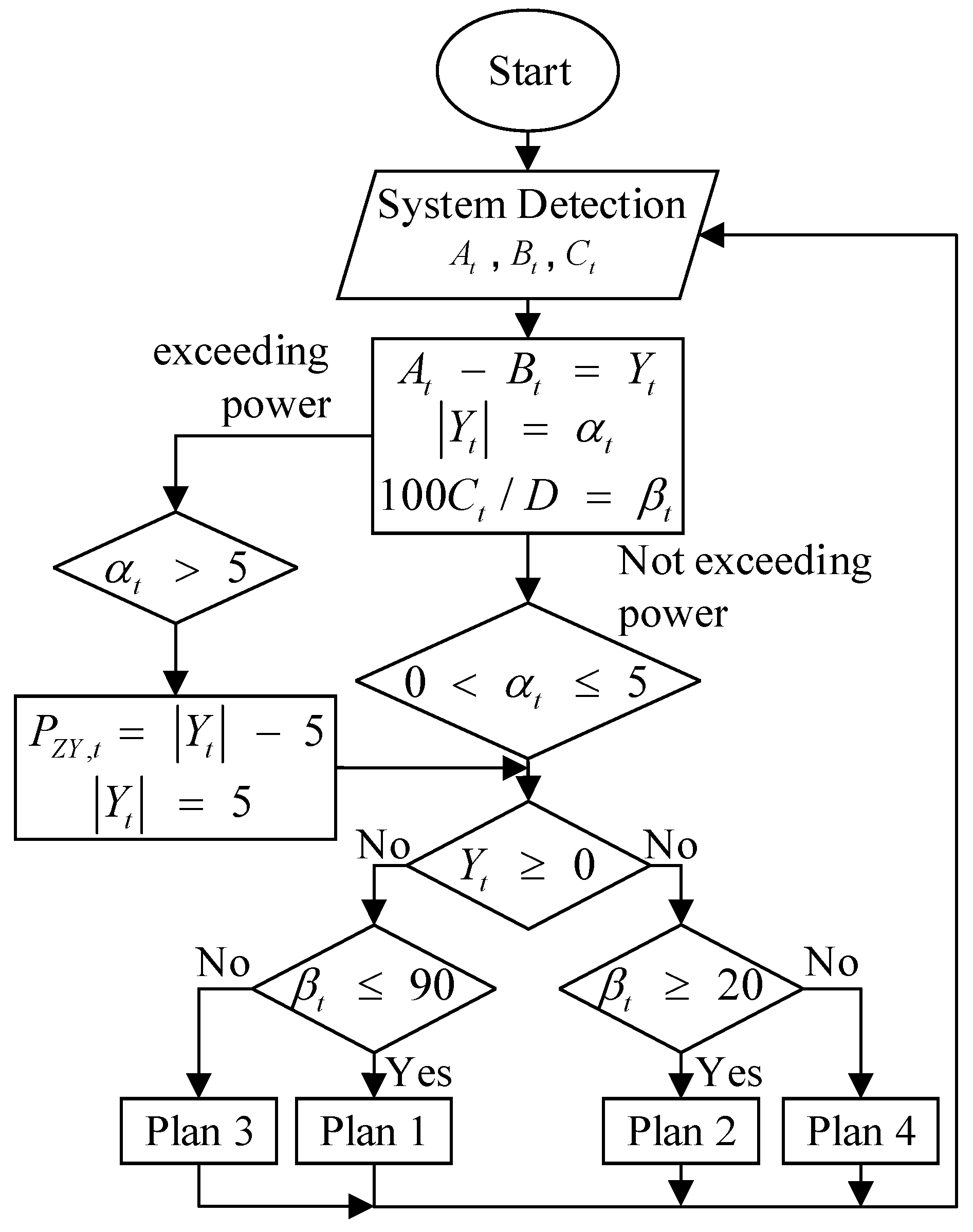
3.2. Intraday Market Adjustment Strategy Model

The intraday adjustment needs a time span of 15 min. When the time span is shorter, a higher precision is achieved for control and adjustment. Based on the trading outcomes of the day-ahead market, the intraday market focuses on the disequilibrium adjustment of intraday differentials. ES and EL are the major entities responsible for these adjustments. ES operates according to the real-time supply and demand under the system load, which ensures excess charging during the periods of surplus supply and discharging when the supply is outstripped by the demand. Differently, EL is responsible for accommodating any excess capacity from WD and PVs on the basis of meeting the demand of the system and grid for energy.

3.2.1. ES Adjustment Strategy Model

The capacity of ES is determined by carefully considering such factors as the historical peak load differential, the duration of this differential, and construction costs. In this study, a peak load differential of 5 MW, sustained for 3 h, is used to calculate the parameter of ES configuration to be 5 MW/15 MW·h.

The real-time capacity of ES [22], denoted as $S_{CN,t}^{RL}$, is calculated using the formula shown in Equation (14).

$$S_{\mathrm{CN},t}^{\mathrm{RL}}=\left(1-{\mu }_{\mathrm{CN}}^{\mathrm{SH}}\right)S_{\mathrm{CN},t-1}^{\mathrm{RL}}+\left({\eta }_{\mathrm{CN}}^{\mathrm{CD}}P{E}_{\mathrm{CN},t}^{\mathrm{CD}}-P{E}_{\mathrm{CN},t}^{\mathrm{FD}}/{\eta }_{\mathrm{CN}}^{\mathrm{FD}}\right)\frac{\Delta t}{C_{\mathrm{CN}}}$$

(14)

where ${\mu }_{\mathrm{CN}}^{\mathrm{SH}}$ represents losses; $S_{\mathrm{CN},t-1}^{\mathrm{RL}}$ is the capacity in the $t-1$-time period, measured in MWh; ${\eta }_{\mathrm{CN}}^{\mathrm{CD}}$ is the charging efficiency; ${\eta }_{\mathrm{CN}}^{\mathrm{FD}}$ is the discharging efficiency; $C_{\mathrm{CN}}$ denotes the energy storage capacity of ES; and $\Delta t$ represents the time period of 15 min. The stress response process of ES is illustrated in Figure 4.

In Figure 4 $A_t$, $B_t$, and $C_t$ represent the real-time system load, the next day execution load, and the real-time capacity of ES, respectively, for the $t$-time period; $Y_t$ represents the difference between the real-time system load and the next day execution load; ${\alpha }_t$ represents the percentage of the difference between the real-time system load and the next day execution load; and ${\beta }_t$ represents the percentage of ES’s real-time capacity relative to the total system capacity.

Plan 1 is that the system charges the ES and issues a load-shedding notification.

Plan 2 is that the ES discharges to the system and issues a load-up notification.

Plan 3 is to trigger the ES overcapacity limit isolation protection and transfer overcharged energy.

Plan 4 is to trigger the ES overcapacity lower limit isolation protection and transfer overdischarged energy.

3.2.2. EL Power Redistribution

The electricity pricing of EL is subject to an upper limit. Its profitability is reduced when this limit is exceeded. Since the price of electricity supplied by WD and PVs to the EL is lower compared to the electricity entering the grid, the stability of electricity supplied to the EL may be compromised to a certain degree for cost-effectiveness. The power predetermined for EL before the day-ahead stage is purposed to match the WD and PVs to determine the power supplied to the system load and to the grid portion. Since these two portions are carried over to the intraday period, the EL receives the remaining portion of the power during the intraday stage. Since the order of power allocation for EL changes in the day-ahead and intraday stages, it is referred to as the “redistribution of power” during the intraday period.

The power obtained by EL from WD and PVs is represented as Equation (15).

$$\{\begin{array}{l}P{E}_{\mathrm{P}2\mathrm{Gfd},t}^{\mathrm{RN}}=P{E}_{\mathrm{FDp},t}^{\mathrm{RN}}-\left(P{E}_{\mathrm{FDp},t}^{\mathrm{RW}}+P{E}_{\mathrm{FDp},t}^{\mathrm{FH}}\right)\\ P{E}_{\mathrm{P}2\mathrm{Ggf},t}^{\mathrm{RN}}=P{E}_{\mathrm{GFp},t}^{\mathrm{RN}}-\left(P{E}_{\mathrm{GFp},t}^{\mathrm{RW}}+P{E}_{\mathrm{GFp},t}^{\mathrm{FH}}\right)\\ P{E}_{\mathrm{P}2\mathrm{G},t}^{\mathrm{RN}}=P{E}_{\mathrm{P}2\mathrm{Gfd},t}^{\mathrm{RN}}+P{E}_{\mathrm{P}2\mathrm{Ggf},t}^{\mathrm{RN}}\end{array}$$

(15)

where $P{E}_{\mathrm{FDp},t}^{\mathrm{RN}}$ and $P{E}_{\mathrm{GFp},t}^{\mathrm{RN}}$ represent the real-time outputs of WD and PVs during the day, respectively. $P{E}_{\mathrm{P}2\mathrm{Gfd},t}^{\mathrm{RN}}$ and $P{E}_{\mathrm{P}2\mathrm{Ggf},t}^{\mathrm{RN}}$ represent the remaining electrical energy received by EL from WD and PVs in real time during the day, respectively, whose sum is denoted as $P{E}_{\mathrm{P}2\mathrm{G},t}^{\mathrm{RN}}$. For further explanations, please refer to Equation (3).

Deviation Reward and Penalty: The deviation denoted as $P{E}_{\mathrm{FDp},t}^{\mathrm{RN}}$ and that denoted as $P{E}_{\mathrm{GFp},t}^{\mathrm{RN}}$ can be either positive or negative. Moreover, there is a possibility that one side contributes positively or the other side is offset when energy is supplied to EL. When one party is the main supplier to EL, EL rewards the other party that contributes positively, while it penalizes the other party that offsets the contribution. The amount of penalty is determined by the maximum peak-valley electricity price of EL. The “assist increase” and “offset” quantities are detailed in the section on EL transaction results.

3.2.3. Incentive for Reserve Capacity Selling

In the context of BGCHP and WICHP, the surplus capacity from the day-ahead stage is treated as backup capacity to compensate for intraday discrepancies. When the backup capacity is involved, the electricity generated is purchased at a price that is 50% higher than the price of the day-ahead transaction.

As consideration is given to operation and maintenance costs, as well as construction expenses in the day-ahead capacity market stage, they are discounted in the intraday stage. The units have become operational since the day-ahead stage, so there is no need to reevaluate them. The incentive for capacity providers to utilize the reserve capacity is expressed as Equation (16).

$$I_{\mathrm{JL}}^{\mathrm{RN}}=\left(Q_{\mathrm{CNSn},t}^{\mathrm{RN}}-Q_{\mathrm{CNSn},t}^{\mathrm{RQ}}\right)\cdot \left(1+0.5\right)e_{\mathrm{CNSn},t}^{\mathrm{RQ}}$$

(16)

where $e_{\mathrm{CNSi},t}^{\mathrm{RQ}}$ represents the capacity transaction price for the nth capacity provider in the day-ahead market in the $t$-time period. $Q_{\mathrm{CNSi},t}^{\mathrm{RQ}}$ and $Q_{\mathrm{CNSi},t}^{\mathrm{RN}}$ respectively, denote the traded electricity volume in the day-ahead market in the $t$-time period and the actual traded volume in the intraday market in the $t$-time period.

4. Model Solving and Simulation Analysis

4.1. Construction and Solving of Electricity Trading Model

In this paper, the term “system load” refers to historical data collected from the general industrial and commercial sector within Shaanxi. The “peak and valley segments” and corresponding pricing information relate to the peak and off-peak periods and charges. Further details can be found in Section 4.2.2—Analysis of electricity transaction price. The parameters required for the power generation units used in this paper are based on the actual output of existing units in Shaanxi, whose values are listed in Appendix C. This paper focuses mainly on the construction of a microgrid system model, as illustrated in Figure 1. The day-ahead transaction model is established using the generic software of mathematical modeling, namely, GAMS 28.2.0. The model constructed in GAMS shows nonlinearity (NLP) due to the constraints on the quadratic term that reflect the relationship between marginal prices and marginal outputs. The model is solved using the built-in solver of GAMS, IPOPT. For the intraday trading component, the ES unit is prioritized. A stress model is established using MATLAB software (MATLAB 2021b) to monitor and assess the outcomes of its trading. To evaluate the results of trading, three comparative scenarios are involved: full capacity fixed-price trading, responsive system load demand bidding trading, and responsive system load demand fixed-price trading.

4.2. Trading Results and Analysis

4.2.1. Results and Analysis of Electricity Trading

(1)

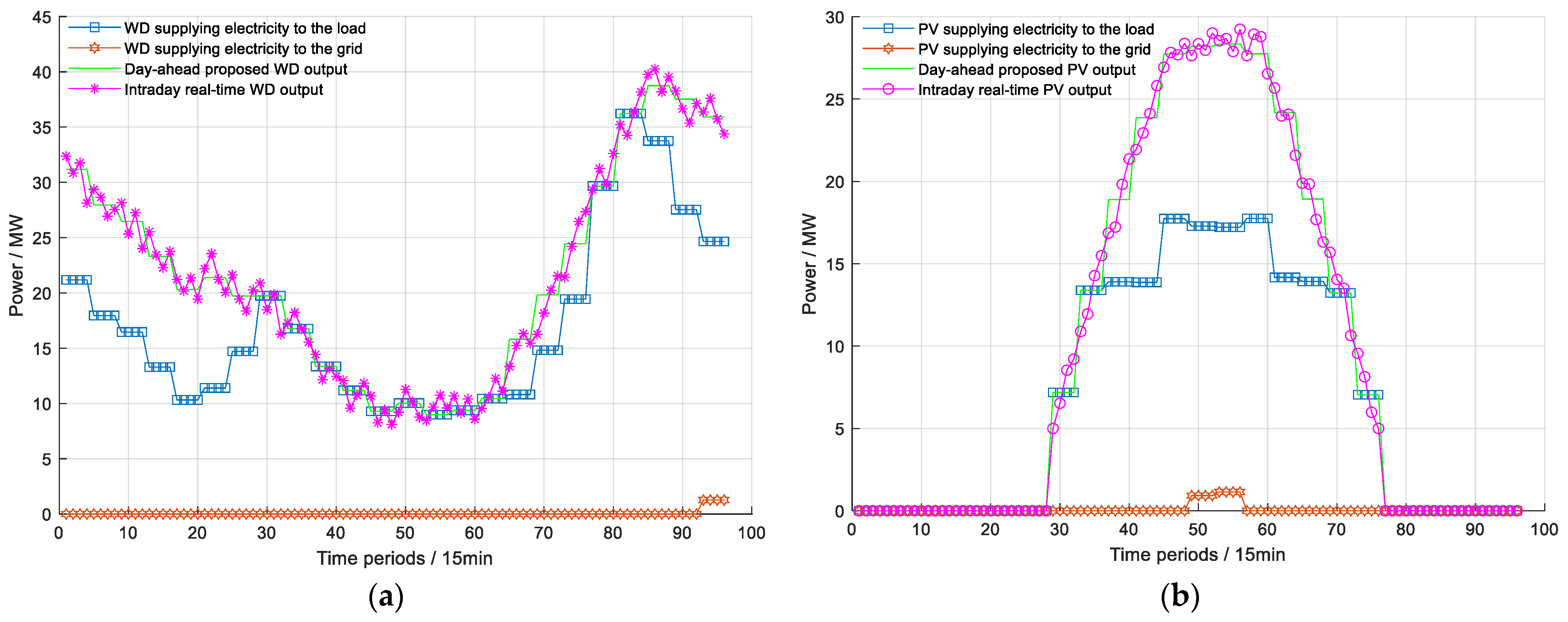
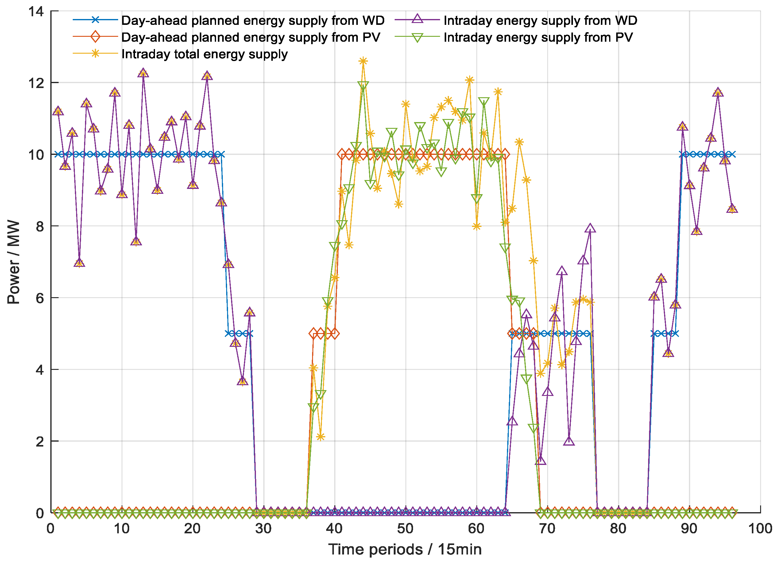
Analysis of WD and PV trading results.

The on-site utilization of electrical energy generated by WD and PV power is depicted in Figure 5 below.

The day-ahead fitted outputs and real-time outputs of WD and PV power are represented by the green and red curves, respectively. The electrical energy supplied to the system load is depicted by the blue curve, while the electrical energy fed to the grid is shown by the orange curve. From the graph, it is evident that the real-time curve closely tracks the day-ahead fitted curve, indicating highly accurate predictions. WD output gradually decreases during the daytime and increases again at night. In contrast, PV output follows the opposite trend, increasing as WD output diminishes. Thus, PV power serves as a complementary source of electricity during the day. Before PV power begins generating electricity, the electrical supply to the system load and EL primarily originates from WD. However, when PV output is substantial, PV power becomes a significant contributor to both the system load and the electrical requirements of EL. The remaining electrical energy needed by the system load is sourced from BGCHP and WICHP.

The real-time outputs of WD and PV power differ to the average trading quantities from the day-ahead market, such as when there is an energy deficit during certain periods and an energy surplus during others. This is considered to be normal, as exemplified during the 30th–33th time periods in Figure 5b. This situation can be controlled by the ES system, which is used to maintain system stability by storing excess energy during surplus periods and then releasing it during deficit periods.

(2)

Analysis of BGCHP and WICHP transaction results.

The trading results for BGCHP and WICHP are depicted in Figure 6 below.

In the 0th–28th time periods, both BGCHP and WICHP gradually increased as WD output decreased. In the 29th–48th time periods, the initial fluctuation was followed by a decrease as the morning peak ended, while PVs gradually began power generation. In the 49th–56th time periods, BGCHP and WICHP operated at their minimum guaranteed power due to excessive PV output. In the 57th–68th time periods, they first increased and then decreased with a decrease in PV output and load. In the 69th–80th time periods, BGCHP and WICHP maintained their output at the end of the 68th period, while their output increased to the maximum as PV output declined significantly. In addition, WD output slowly recovered, and the system load peaked. In the 77th–80th time periods, there was a shortage of internal supply within the system due to the system load approaching its peak. Thus, the upstream grid supplied 1.01 MW to the system. In the 81th–96th time periods, the system load peaked before a decline. Meanwhile, BGCHP and WICHP gradually reduced their output until operating at their minimum guaranteed power.

Since the marginal price of WICHP remains lower compared to BGCHP, WICHP consistently exhibits a slightly higher output power than BGCHP in each trading session. However, it is worth noting that the output power of both BGCHP and WICHP was restricted by the maximum output power of PVs during the 49th–56th time periods. Similarly, BGCHP and WICHP were constrained during the 93th–96th time periods, which was due to a significant reduction in system load and the high output from WD.

As for the use of standby capacity, BGCHP increased by 1.511 MW and 0.329 MW in the 30th and 93rd periods, respectively. Likewise, WICHP added 1.559 MW and 0.381 MW in the 30th and 93rd periods, respectively.

(3)

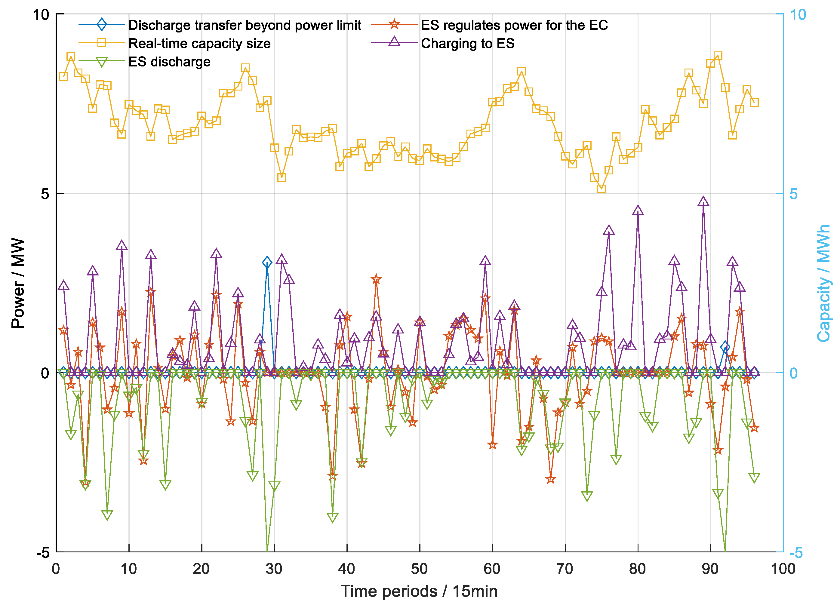
Analysis of ES transaction results.

ES’s intraday adjustments are illustrated in Figure 7 below.

From ES adjustments, it can be observed that the charging and discharging power of ES are mostly below 4 MW, which is lower than the rated 5 MW, indicating that the grid operator’s day-ahead forecast of system load demand closely aligns with the real-time load demand. However, there are instances of overpower discharge transfers in the 30th and 93rd time periods, with transfer powers of 3.07 MW and 0.71 MW, respectively, provided by BGCHP and WICHP. There were no occurrences of overcapacity charging or discharging and overpower charging, so they are not shown. The inlet capacity of the ES has an average value of 7.526 MWh and operates below its standard storage capacity of 8.250 MWh. However, the charge/discharge capacity at the outlet end is 6.941 MWh on average, suggesting that the ES experiences some losses during the normal charge/discharge process.

Because the electricity supply to the EL becomes unstable after redistribution, it is necessary to use the ES for power supply stabilization to the EL. The stabilization curve of the ES for the EL is depicted by the green curve.

(4)

Analysis of EL trading results.

EL in this system plays the role of an energy recipient for the surplus power generated by WD and PVs. It also serves as a regulator for the system’s load. The trading results of EL for both the day-ahead and intraday markets are illustrated in Figure 8.

According to the EL trading results, the proposed WD power supplied to EL at this time is 10 MW/h in both the 0th–24th and 89th–96th time periods, which is due to the high WD output and limited system load. However, the power it receives after intraday reallocation fluctuates at around 10 MW/h, and it is still ensured that the EL operates close to full capacity during that time period. During the 25th–28th time periods, when the WD output gradually decreases, the power supplied to the EL declines. In spite of this, 5 MW/h of power supply remains. In the 29th–36th time periods, the power supplied to EL is zero because the power supply to the system load is prioritized, given the continued low WD output and an early peak in the system load. During the 77th–88th time periods, the EL receives no power supply due to an evening peak that the system load experiences, and the power supply to the system load is prioritized. In the 37th–64th time periods, PVs becomes the primary source of power supply for EL, and WD surplus power increases the supply of PVs to EL, which boost or offset each other. For example, in the 37th time period, the surplus power of WD increases the supply of PVs, resulting in a higher amount than expected. In contrast, in the 38th time period, the surplus power of WD offsets the supply of PVs, resulting in a lower amount than expected. In the 37th–64th time periods, PVs is the primary source of power supply for EL, while the surplus power from WD either enhances or offsets the power supplied by PVs to EL. For instance, in the 37th time period, it enhances the power supply and is higher than the actual one. Conversely, in the 38th time period, it offsets the power supply and is lower than the actual one.

In the 65th–68th time periods, both WD and PVs supply power to EL simultaneously without causing interference with each other. During the 69th–76th time periods, WD once again becomes the primary source of power supply for EL. However, the remaining proportion of power supplied by PVs either enhances or offsets this power supply.

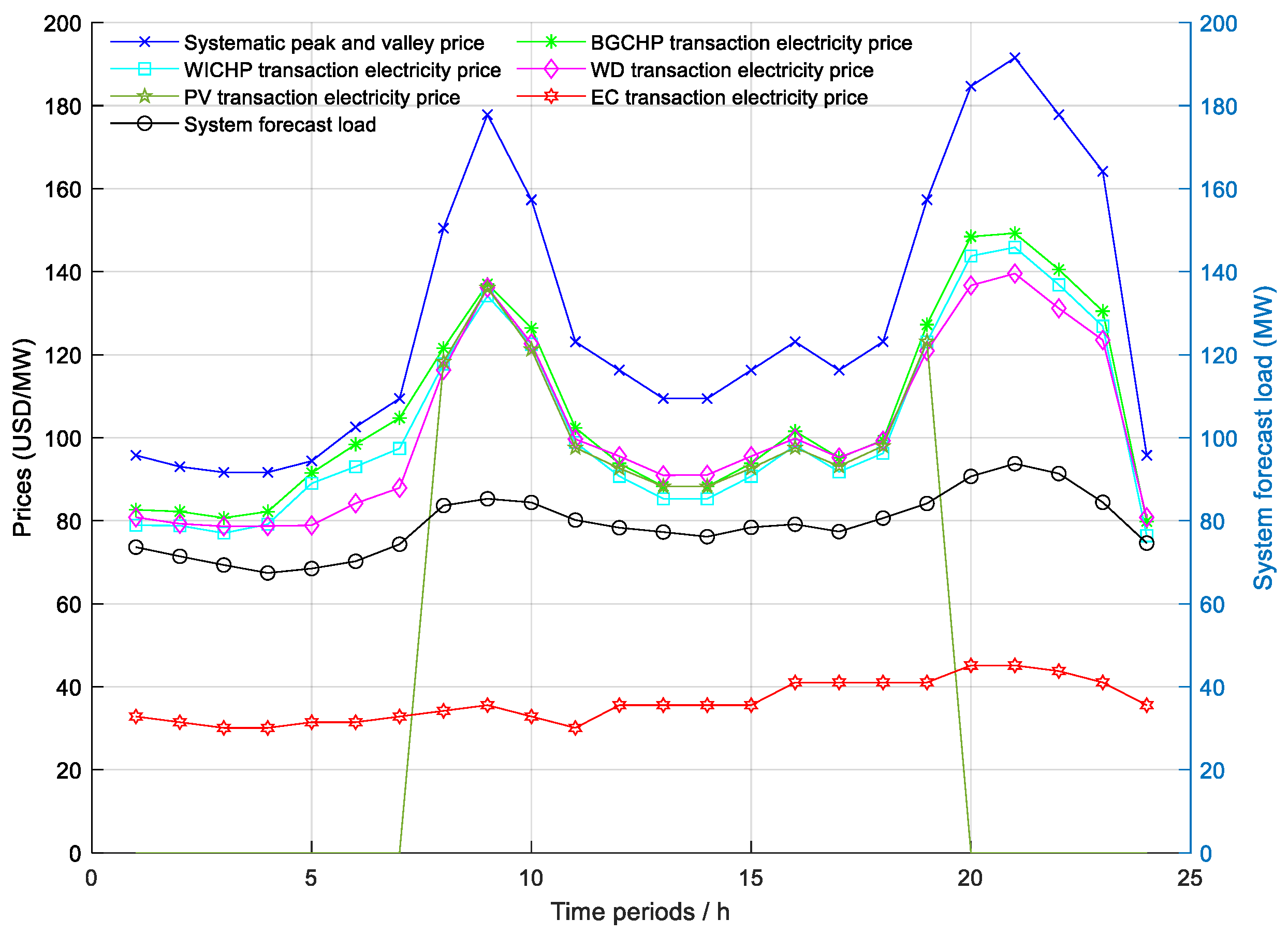
4.2.2. Analysis of Electricity Transaction Price

The transaction price of electricity is shown in Figure 9 below.

During a typical summer day, the time periods from 0:00 to 7:00 and 23:00 to 0:00 constitute the valley periods, while 10:00 to 18:00 represents the flat period. The hours from 19:00 to 22:00 are considered the spike periods, with the remaining hours classified as peak periods.

The electricity transaction prices for each capacity unit are affected by the peak and off-peak tariffs of the system, suggesting that the mechanism of pricing intervention influences the capacity of the capacity provider through price signals. Moreover, all transaction prices exceed their marginal costs, thus ensuring the generation of revenues.

4.2.3. Analysis of Revenue Generated from Electrical Energy

(1)

Analysis of trading volume and revenue.

The trading volume and profits for capacity providers and operators are summarized in

Table 1. Bilateral trading table.

Project Title	Scenarios	Electricity Traded (MWh)	Energy Gains (USD)	Fuel Costs (USD)	O&M Cost (USD)	Heat Traded (t/h)
BGCHP	1	720.000	73,872.000	29,548.800	3447.360
	2	655.489	70,118.208	26,897.616	3138.192	1716.580
	3	655.489	67,253.616	26,897.616	3138.192
WICHP	1	720.000	64,022.400	20,827.800	3348.864
	2	660.132	68,114.088	19,095.912	3069.792	1131.736
	3	660.132	58,698.144	19,095.912	3069.792
WD	1	517.443	33,269.760	0	2123.136
	2	411.390	44,213.760	0	2123.136
	3	411.390	26,450.280	0	2123.136
PV	1	238.140	14,008.320	0	846.792
	2	166.700	16,887.960	0	846.792
	3	166.700	9805.824	0	846.792
Operator	2	1894.700	47,044.152	0	33,732.144

:

Scenario 1 is the ideal one where full-capacity power generation is achieved without any response to the changes in system demand. It is characterized by fixed-price trading. Scenario 2 shows the participation in market-based trading, where transactions are conducted through the competition on price and volume to meet system demand. This scenario is the focus of this study. Scenario 3 is a common one where power generation adapts to system load demand but still involves fixed-price trading without the involvement of market-based mechanisms.

As revealed by an analysis of the electric energy gains of BGCHP, the electric energy gain is USD 3794.832 lower in Scenario 2 than in Scenario 1 on a typical day. To a large degree, this difference is attributed to the higher turnover in Scenario 1. In Scenario 2, the generation of power is lower due to the system load demand, which may lead to less gain. After the fuel cost and O&M cost are deducted, the net profit in Scenario 1 amounts to approximately USD 40,875.840, while a net profit of USD 40,082.400 is generated in Scenario 2. The daily net income under both scenarios is highly similar, but the net income from participating in market-based trading remains slightly lower than from the full-issue subsidy offered for entry into the grid. If the amount of straw consumed by BGCHP in Scenario 1 with an annual operating length of 5500 h [6] is taken as the benchmark, the annual net profit is USD 9,360,567.360 and USD 10,000,607.110 in Scenario 1 and Scenario 2, respectively. This means a recovery of annual net profit, which is USD 700,143.768 higher in Scenario 2 than in Scenario 1. This is equivalent to an increase by USD 2789.352 in net profit for each trading day, which is attributed to the reduction in straw consumption after the participation in market-based trading. This reduction extends the total number of hours of electricity supply, thus improving profitability. When compared with Scenario 3, an additional USD 2864.592 is generated in net revenue. Considering that industrial steam is priced at USD 19.152 per ton in Shaanxi, the daily steam net profit gained by BGCHP is USD 28,414.728, which accounts for 70.7% of the net profit from electricity sales. It is clearly demonstrated that cogeneration can significantly boost incomes.

The electricity revenue situation for WICHP is considerably more favorable compared to BGCHP. In a typical day, Scenario 2 generates USD 4091.688 more in daily revenue than the situation in Scenario 1, where fixed capacity is fed to the grid at a fixed price. After deducting fuel and operational costs, the daily net profit amounts to USD 46,034.568. When added to the cost of the reserve capacity call, the net benefit is USD 2097.144 higher than that of Scenario 1. Compared to Scenario 3, there is an additional revenue of USD 9415.944. It can be observed that WICHP generates revenue somewhat easier compared to BGCHP. Additionally, the daily net revenue of USD 18,733.392 generated by WICHP from steam, after accounting for heat net access and desalting costs, is also a significant source of revenue.

WD and PV power are comparable to WICHP in terms of profitability, which increases revenue directly when compared to Scenario 1. After the deduction of power supply incentives and penalties to EL, as well as O&M costs, WD generates a net profit of USD 45,706.248, while PV power generates a net profit of USD 18,492.624.

The revenue generated by the operator is USD 47,044.152. Moreover, after the deduction of USD 33,732.144 spent on ES, the daily net profit reaches USD 13,310.64. ES processes 40.627 MWh of electricity on a daily basis, which is equivalent to a cost of 8.081 cents/kWh for ES electricity processing.

(2)

Comparative analysis.

In the case of BGCHP, the fixed-price trading strategy [8] is similar to that under Scenario 3 in this paper, with the trading price fixed at 10.260 cents/kWh. Conversely, the trading strategy applied in this paper extends the number of supply days for BGCHP from 229 to 251, and the transaction price is mostly higher than this fixed price. Therefore, the market-based trading approach can be taken to enhance the sustainability of BGCHP.

In the case of WICHP, using the fixed-price trading method at 8.892 cents/kWh [12], the annual net profit for cogeneration amounts to USD 20,028,983.760. However, in this paper, with the microgrid system comprised entirely of renewable energy sources participating in market-based trading, the annual net profit stands at USD 21,589,324.56, which is an additional USD 1,560,327.120. It can be seen that the participation in market-based trading can significantly improve the earnings.

In the previous research on WD and PV power generation [8,9], wind or solar energy curtailment is an issue that is commonly encountered. In this paper, EL is introduced to optimize the efficiency of WD and PV utilization by ensuring that excess power is absorbed for idling when power generation is insufficient. This strategy aims to prevent the wastage of energy resulting from the abandonment of wind or solar power. Furthermore, market-based bidding trading is proposed in this paper for WD and PV power generation, which causes the transaction prices to exceed the rates for “over-the-wall electricity sales”, thus creating significant economic benefits.

5. Conclusions

In this paper, an in-depth analysis is conducted on both challenges and solutions concerning the survival and profitability of BGCHP, given its withdrawal from government subsidies. To ensure survival, two primary strategies are proposed. Firstly, it is recommended to shift from a singular electricity generation model to a CHP model for the diversification of revenues. Secondly, it is suggested to establish a multi-energy, mutually supportive microgrid system in collaboration with WD and PV sources. This integrated system is designed to ensure stable and dependable energy supply for commercial and industrial users. To address the challenge in profitability, a market-oriented trading strategy is introduced in this paper. This strategy involves a dual mechanism, including a guaranteed minimum level of electricity generation and transactions when prices exceed marginal costs, thus guaranteeing revenues.

Through simulation, the following conclusions are reached:

• In this study, the microgrid system, comprised completely of renewable energy sources, operates in a mode of “self-generation and self-consumption, electricity surplus sales, electricity shortfall purchase”. There is an exceptional situation that energy is purchased from the higher grid once, power is generated at full capacity twice, and operation is conducted under the minimum guaranteed power three times. Additionally, the power generated by WD and PVs is rarely supplied to the grid. Instead, the excess capacity is efficiently incorporated by the EL, thus eliminating the possibility of any excess capacity being wasted due to wind and sunlight. It is demonstrated that the capacity configuration proposed in this paper satisfies the requirements on system load, which ensures that BGCHP and WICHP can generate power within a reasonable range. Meanwhile, the utilization of all electricity generated by WD and PVs is maximized.
• The trading strategy proposed in this paper aligns with the trend of market-oriented reforms, ensuring that significantly higher economic returns are generated for all capacity units involved in market-based trading. For instance, BGCHP and WICHP guarantee a daily net profit that is USD 2864.592 and USD 9415.944 higher than in Scenario 3, respectively. WD and PVs can also generate an additional USD 17,763.480 and USD 7082.136 per day in revenue, respectively, when compared to Scenario 3. Additionally, the operator records substantial daily net profits of USD 13,313.376.
• The ES system introduced in this paper enables the prompt adjustment made by the systems to load supply and demand, which facilitates system operations. Moreover, it enhances the stability of electrical energy supply for EL. Although a lower ES capacity has the potential to boost revenues for the operator, it may not be conducive to ensuring system stability.
• An innovative market-based trading concept is introduced for the microgrids comprised entirely of renewable energy sources. It aims to create a multi-energy complementary energy supply portfolio that improves the capacity and profitability of the power supply.

Notably, the scope of application as discussed in this paper mainly includes the general industrial and commercial energy sectors, rather than large-scale industrial or residential uses. In the former setting, a substantial amount of electricity is typically consumed and there may be challenges in the supply capacity of the system. Conversely, the latter often shows scattered energy consumption and lower energy prices, which potentially affects the profitability of this capacity unit. Additionally, this paper focuses on optimizing electrical energy, instead of the classification and optimization of thermal energy usage. In future research, it is worth considering the classification of system load and energy use for modeling and simulating its optimization, so as to further reduce energy costs.

References

1. Han, G.; Zhou, Z. Summary of Development Status of Incremental Distribution Network and Research on Development Trend. China Water Power Electrif. 2022, 204, 46–50. [Google Scholar]
2. Wang, X. New power system to build a new ecology of source-grid-load-storage. Energy 2021, 7, 28–30. [Google Scholar]
3. Yu, D.; Zhang, C.; Wang, S.; Zhang, L. Evolutionary Game and Simulation Analysis of Power Plant and Government Behavior Strategies in the Coupled Power Generation Industry of Agricultural and Forestry Biomass and Coal. Energies 2023, 16, 1553. [Google Scholar] [CrossRef]
4. Fu, P.; Xu, G.; Li, X.; Zhu, T.; Zhang, Z. Analysis of the Development Status and Trends of China’s Biomass Power Industry and Carbon Emission Reduction Potential. Ind. Saf. Environ. Prot. 2021, 47, 48–52. [Google Scholar]
5. Zhu, X.; Dou, K.; Wang, Z. Economic Analysis of China’ s Agricultural and Forestry Biomass Power Generation Projects. J. Glob. Energy Interconnect. 2022, 5, 182–187. [Google Scholar]
6. Illankoon, W.A.M.A.N.; Milanese, C.; Girella, A.; Rathnasiri, P.G.; Sudesh, K.H.M.; Llamas, M.M.; Collivignarelli, M.C.; Sorlini, S. Agricultural Biomass-Based Power Generation Potential in Sri Lanka: A Techno-Economic Analysis. Energies 2022, 15, 8984. [Google Scholar] [CrossRef]
7. Lin, X.; Wu, Y. Thermodynamic Simulation and Analysis of Biomass Gasification Cogeneration System. J. Eng. Therm. Energy Power 2019, 34, 15–22. [Google Scholar]
8. Li, S.; Liu, Z.; Wang, J.; Liu, W.; Guo, H. Two-stage operation optimization of rural biomass energy integrated energy system considering heat network loss. Electr. Power Autom. Equip. 2021, 41, 24–32. [Google Scholar]
9. Bagherian, M.A.; Mehranzamir, K.; Rezania, S.; Abdul-Malek, Z.; Pour, A.B.; Alizadeh, S.M. Analyzing Utilization of Biomass in Combined Heat and Power and Combined Cooling, Heating, and Power Systems. Processes 2021, 9, 1002. [Google Scholar] [CrossRef]
10. Indrawan, N.; Simkins, B.; Kumar, A.; Huhnke, R.L. Economics of Distributed Power Generation via Gasification of Biomass and Municipal Solid Waste. Energies 2020, 13, 3703. [Google Scholar] [CrossRef]
11. Baeyens, E.; Bitar, E.Y.; Khargonekar, P.P.; Poolla, K. Coalitional aggregation of wind power. IEEE Trans. Power Syst. 2013, 28, 3774–3784. [Google Scholar] [CrossRef]
12. Smale, R.; Spaargaren, G.; van Vliet, B. Householders co-managing energy systems: Space for collaboration. Build. Res. Inf. 2019, 47, 585–597. [Google Scholar] [CrossRef]
13. Huang, W.; Ge, W.; Ren, H.; Zhu, Y.; Chen, H. Exploration of optimal configuration and operation for all-renewable multi-energy complementary systems. J. Acta Energiae Solaris Sin. 2023, 11–25. [Google Scholar]
14. Wang, X.; Ren, H.; Wu, Q.; Li, Q. Research on Optimal Planning Method of Multi-source Heterogeneous All-renewable Energy System facing Carbon Neutrality. J. Eng. Therm. Energy Power 2022, 37, 136–145. [Google Scholar]
15. Zhong, W.; Pan, X.; Fan, W.; Zhang, J.; Zhou, R. Energy Efficiency Optimization of Waste Incineration Power Plant with Waste Heat Recovery Device and Compression Heat Pump. Proc. CSU-EPSA 2021, 33, 117–124. [Google Scholar]
16. Zhang, Y.; Zhao, N.; Huang, J.; Bu, G. Two-level coordinated operation optimization model of the source-storage-load in microgrid considering demand response. Energy Res. Inf. 2020, 36, 216–221. [Google Scholar]
17. Zhao, R.; Tan, Z.; Degjirif, U. A two-level coordinated operation optimisation model of microgrid “source-storage-load” taking into account demand response. Renew. Energy Resour. 2019, 37, 1630–1636. [Google Scholar]
18. Qian, C.; Bao, H. Unscrambling of marginal cost algorithm in power market. Power Syst. Prot. Control. 2010, 38, 7–10+15. [Google Scholar]
19. Yu, J. Study on Competitive Bidding Strategy of Power Plant Based on Marginal Generating Cost Analysis; Shandong University: Jinan, China, 2015. [Google Scholar]
20. Wang, Y.; Wang, X.; Sun, Q.; Zhang, Y.; Liu, J.; Jinghan, H.E. Multi-agent Real-time Collaborative Optimization Strategy for Integrated Energy System Group Based on Energy Sharing. Autom. Electr. Power Syst. 2022, 46, 56–65. [Google Scholar]
21. Lin, X.; Zhang, Y.; Chen, B.; Fan, S.; Chen, Z. Bi-level Optimal Configuration of Park Energy Internet Considering Multiple Evaluation Indicators. Autom. Electr. Power Syst. 2019, 43, 8–15+30. [Google Scholar]
22. Kumar, P.P.; Nuvvula, R.S.S.; Hossain, M.A.; Shezan, S.A.; Suresh, V.; Jasinski, M.; Gono, R.; Leonowicz, Z. Optimal Operation of an Integrated Hybrid Renewable Energy System with Demand-Side Management in a Rural Context. Energies 2022, 15, 5176. [Google Scholar] [CrossRef]
Figure 1. Microgrid system.
Energies 16 07830 g001
Figure 2. Price intervention curves for system loads.
Energies 16 07830 g002
Figure 3. Curve chart of production capacity supplier quotation.
Energies 16 07830 g003
Figure 4. Mechanism of electrical energy storage stress.
Energies 16 07830 g004
Figure 5. (a) On-site utilization of wind power; (b) On-site utilization of photovoltaic power.
Energies 16 07830 g005
Figure 6. Transaction results of BGCHP and WICHP.
Energies 16 07830 g006
Figure 7. Daily regulation of electric energy storage.
Energies 16 07830 g007
Figure 8. Electrolysis cells’ transaction results.
Energies 16 07830 g008
Figure 9. Electricity transaction price.
Energies 16 07830 g009