

Investigation of Energy Consumption via an Equivalent Thermal Resistance-Capacitance Model for a Northern Rural Residence

 ,
,
Abstract
:1. Introduction
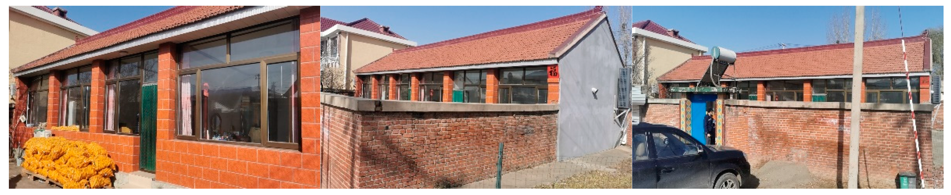
2. Experimental Methodologies
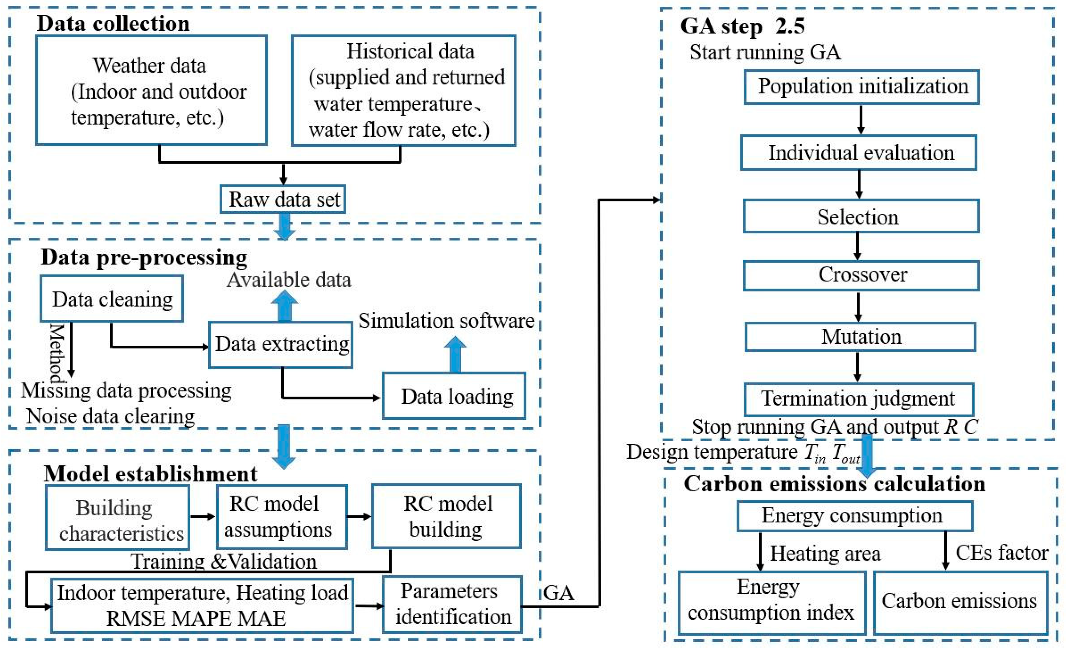
3. Modeling and Methodology
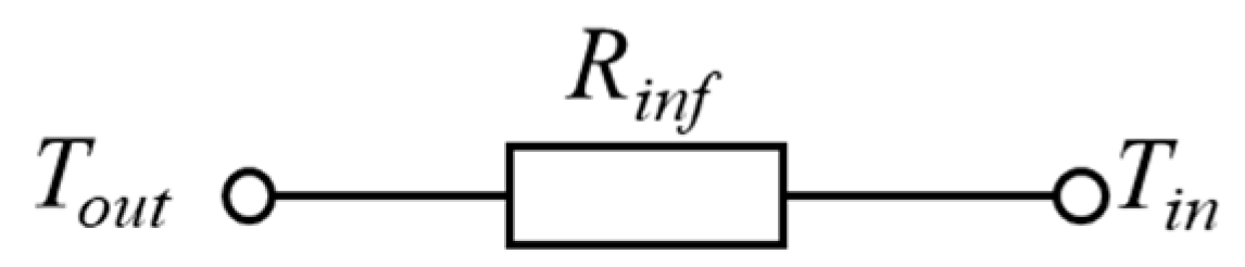
3.1. RC Structure (Assumptions and RC Model)
- (1)
- Heat transfer between indoor and outdoor air through an opaque envelope
- (2)
- Heat transfer through the transparent envelope
- (3)
- Heat transfer from internal heat source and energy supply system
- (4)
- Indoor air and internal thermal mass
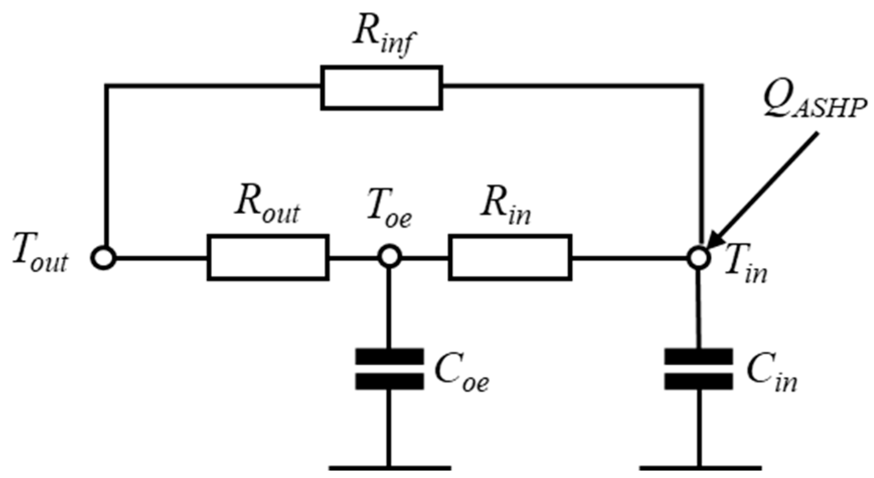
3.2. Equivalent RC Model for Rural Residence
- (1)
- Heat generation or accumulation within the house construction elements does not exist. The temperature of surface segment or whole surface is uniform within its cross section. Thus, the heat transfer can be regarded as a one-dimensional process.
- (2)
- The effect of meteorological parameters, including wind velocity, on heat transfer is negligible. Hence, the thermal resistance or heat transfer coefficient is assumed to be constant. On the side, the effect of temperature and humidity on thermal capacity is not considered; the related thermal capacitance is assumed to be constant.
- (3)
- The experiment is carried out during the night, so the heat from solar radiation or internal heat source is negligible. Hence, the surface temperature of internal thermal mass is assumed to be equal to the indoor air temperature. Correspondingly, the thermal capacitance of the internal thermal mass is summarized to indoor air capacity.
- (4)
- Indoor air is well mixed and homogeneous, so it is assumed to be at a uniform temperature.
3.3. Evaluation Indexes
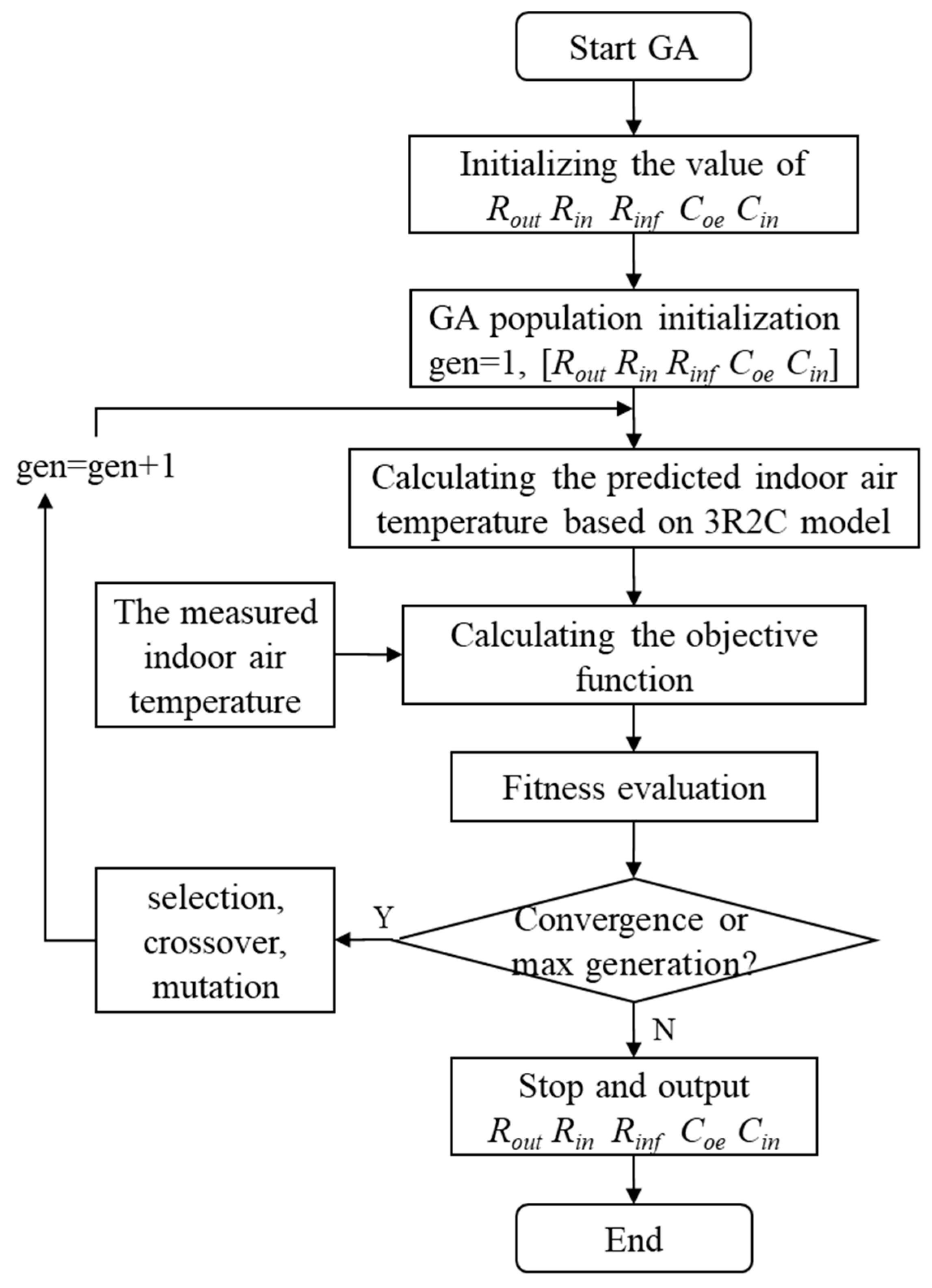
3.4. Optimization Method
3.5. Model of Carbon Emissions
4. Results and Discussion
4.1. Training Results
4.2. Validation Results in the Same Operation Period
4.3. Validated Results in Other Operation Periods
4.4. Estimation of Energy Consumption
4.5. Estimation of Carbon Emissions
4.6. Limitations and Future Research
5. Conclusions
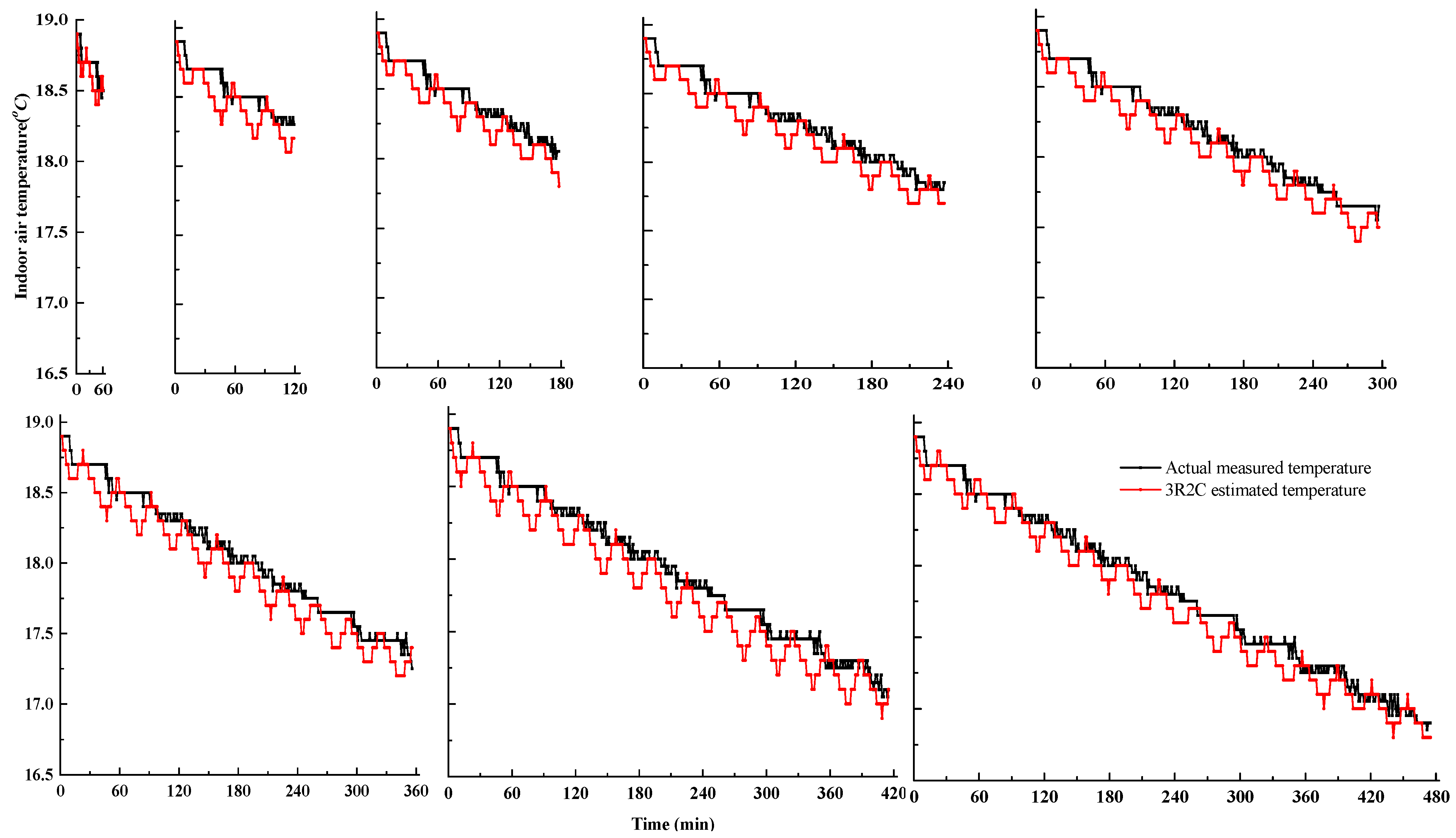
- (1)
- With increasing training time, better following quality between predicted indoor air temperature and actual measured temperature is obtained. When the training time increases to eight hours from one hour, the correlation coefficient increases to 95.45% from 63.15%. The minimum MAE, MAPE, and RMSE values are obtained by training of eight hours, which are 9.79%, 0.55%, and 12.26%, respectively.
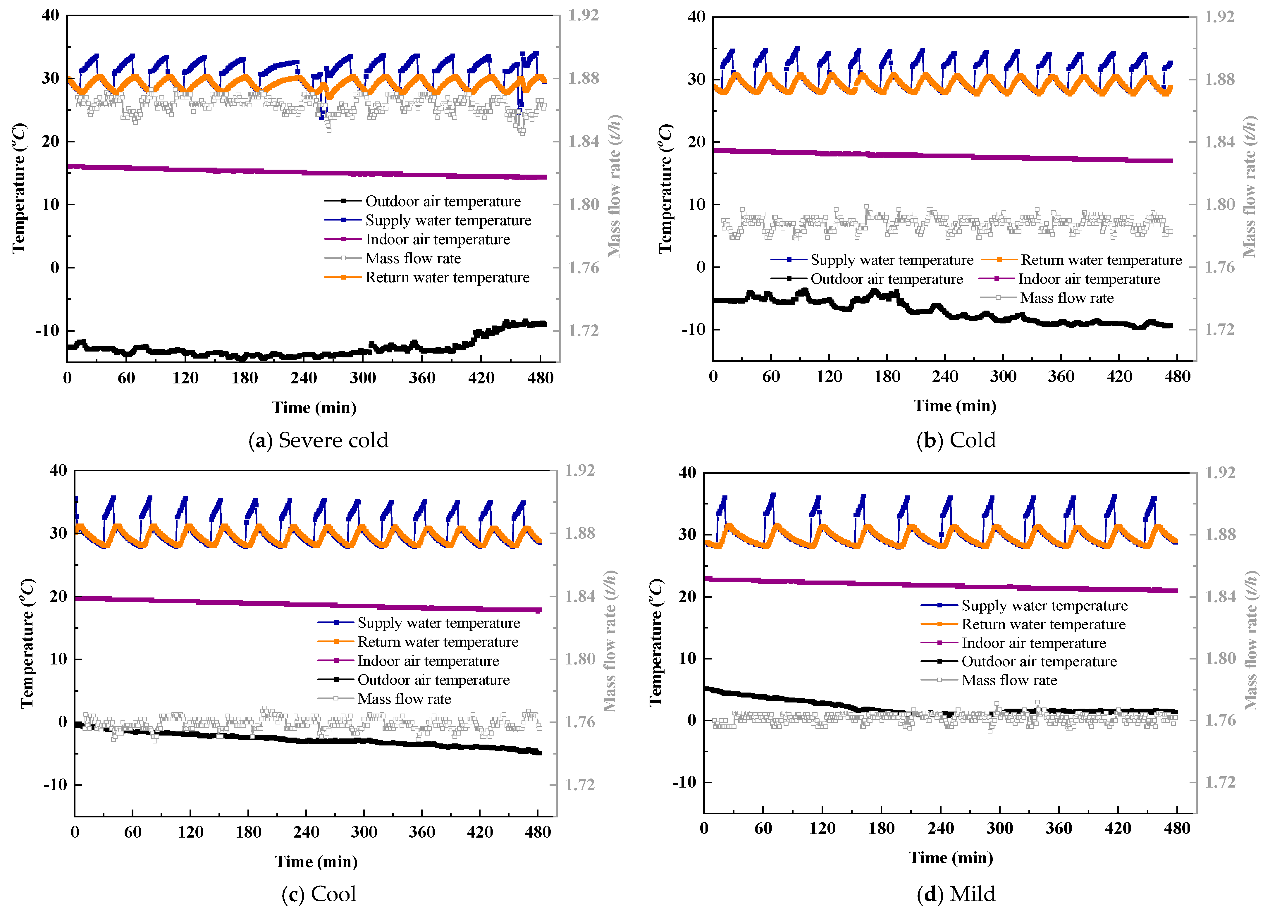
- (2)
- Validation test results of the other four different periods show that regardless of the weather condition, the correlation coefficient is beyond 96%, and the covariance is more than 20%. Under severe cold, cold, cool, and mild weather, RMSE values are 17.91%, 19.71%, 23.32%, and 12.53%, respectively.
- (3)
- A method of estimating carbon emissions and energy consumption is proposed based on the established RC model. The energy consumption index per unit area under standard weather conditions in Beijing can be derived, and it is 46.77 W/m2. Meanwhile, the carbon emissions per unit area values of ASHP, gas boiler, and coal boiler during the entire heating season are 14.6 kgCO2/m2, 12.5 kgCO2/m2, and 44.9 kgCO2/m2, respectively.
Author Contributions
Funding
Data Availability Statement
Conflicts of Interest
Nomenclature
| A | building heating area |
| C | Thermal capacitance |
| CE | total carbon emissions |
| CE0 | carbon emissions per unit aera |
| CEF | carbon emission factor |
| COP | coefficient of performance |
| m | mass flow rate of water |
| P | power consumption |
| Q | nominal heating capacity |
| R | thermal resistance |
| T | temperature |
| density | |
| cp | specific heat |
| Subscripts and Superscripts | |
| in | indoor air |
| inf | infiltration |
| m | internal thermal mass |
| oe | opaque envelope |
| out | outdoor air |
| r | return water |
| s | supply water |
| Abbreviations | |
| ASHP | air source heat pump |
| BIM | building information modeling |
| GA | genetic algorithm |
| MAE | mean absolute error |
| MAPE | mean absolute percentage error |
| RC | model resistance-capacitance model |
| RMSE | root-mean square error |
References
- Norouziasl, S.; Jafari, A. Identifying the most influential parameters in predicting lighting energy consumption in office buildings using data-driven method. J. Build. Eng. 2023, 72, 106590. [Google Scholar] [CrossRef]
- Kang, L.; Wang, J.; Yuan, X.; Cao, Z.; Yang, Y.; Deng, S.; Zhao, J.; Wang, Y. Research on energy management of integrated energy system coupled with organic Rankine cycle and power to gas. Energy Convers. Manag. 2023, 287, 117117. [Google Scholar] [CrossRef]
- Liang, X.; Chen, S.; Zhu, X.; Jin, X.; Du, Z. Domain knowledge decomposition of building energy consumption and a hybrid data-driven model for 24-h ahead predictions. Appl. Energy 2023, 344, 121244. [Google Scholar] [CrossRef]
- Tadeu, S.; Rodrigues, C.; Marques, P.; Freire, F. Eco-efficiency to support selection of energy conservation measures for buildings: A life-cycle approach. J. Build. Eng. 2022, 61, 105142. [Google Scholar] [CrossRef]
- Luo, X.; Ren, M.; Zhao, J.; Wang, Z.; Ge, J.; Gao, W. Study on the life-cycle carbon emission and energy-efficiency management of the large-scale public buildings in Hangzhou, China. J. Clean. Prod. 2022, 367, 132930. [Google Scholar] [CrossRef]
- Xu, Y.; Yan, C.; Wang, G.; Shi, J.; Sheng, K.; Li, J.; Jiang, Y. Optimization research on energy-saving and life-cycle decarbonization retrofitting of existing school buildings: A case study of a school in Nanjing. Sol. Energy 2023, 254, 54–66. [Google Scholar] [CrossRef]
- Oscar, O.; Castells, F.; Sonnemann, G. Life cycle assessment of two dwellings: One in Spain, a developed country, and one in Colombia, a country under development. Sci. Total Environ. 2010, 408, 2435–2443. [Google Scholar]
- Biswas, W.; Wahidul, K. Carbon footprint and embodied energy consumption assessment of building construction works in Western Australia. Int. J. Sustain. Built Environ. 2014, 3, 179–186. [Google Scholar] [CrossRef]
- Luo, X.; Oyedele, L. A data-driven life-cycle optimisation approach for building retrofitting: A comprehensive assessment on economy, energy and environment. J. Build. Eng. 2021, 43, 102934. [Google Scholar] [CrossRef]
- Kneifel, J. Life-cycle carbon and cost analysis of energy efficiency measures in new commercial buildings. Energy Build. 2010, 42, 333–340. [Google Scholar] [CrossRef]
- Rabani, M.; Madessa, H.B.; Ljungström, M.; Aamodt, L.; Løvvold, S.; Nord, N. Life cycle analysis of GHG emissions from the building retrofitting: The case of a Norwegian office building. Build. Environ. 2021, 204, 108159. [Google Scholar] [CrossRef]
- Zhang, Y.; Jiang, X.; Cui, C.; Skitmore, M. BIM-based approach for the integrated assessment of life cycle carbon emission intensity and life cycle costs. Build. Environ. 2022, 226, 109691. [Google Scholar] [CrossRef]
- Peng, C. Calculation of a building’s life cycle carbon emissions based on Ecotect and building information modeling. J. Clean. Prod. 2016, 112, 453–465. [Google Scholar] [CrossRef]
- Liang, Y.; Pan, Y.; Yuan, X.; Yang, Y.; Fu, L.; Li, J.; Sun, T.; Huang, Z.; Kosonen, R. Assessment of operational carbon emission reduction of energy conservation measures for commercial buildings: Model development. Energy Build. 2022, 268, 112189. [Google Scholar] [CrossRef]
- Zhang, C.; Luo, H. Research on carbon emission peak prediction and path of China’s public buildings: Scenario analysis based on LEAP model. Energy Build. 2023, 289, 113053. [Google Scholar] [CrossRef]
- Verbeeck, G.; Hens, H. Life cycle inventory of buildings: A calculation method. Build. Environ. 2010, 45, 1037–1041. [Google Scholar] [CrossRef]
- Shao, L.; Chen, G.; Chen, Z.; Guo, S.; Han, M.; Zhang, B.; Hayat, T.; Alsaedi, A.; Ahmad, B. Systems accounting for energy consumption and carbon emission by building. Commun. Nonlinear Sci. Numer. Simul. 2014, 19, 1859–1873. [Google Scholar] [CrossRef]
- Iddon, C.; Firth, S. Embodied and operational energy for new-build housing: A case study of construction methods in the UK. Energy Build. 2013, 67, 479–488. [Google Scholar] [CrossRef]
- Zhang, Z.; Wang, B. Research on the life-cycle CO2 emission of China’s construction sector. Energy Build. 2016, 112, 244–255. [Google Scholar] [CrossRef]
- Zhu, W.; Feng, W.; Li, X.; Zhang, Z. Analysis of the embodied carbon dioxide in the building sector: A case of China. J. Clean. Prod. 2020, 269, 122438. [Google Scholar] [CrossRef]
- Gan, V.J.; Cheng, J.C.; Lo, I.M.; Chan, C. Developing a CO2-e accounting method for quantification and analysis of embodied carbon in high-rise buildings. J. Clean. Prod. 2017, 141, 825–836. [Google Scholar] [CrossRef]
- Mao, X.; Wang, L.; Li, J.; Quan, X.; Wu, T. Comparison of regression models for estimation of carbon emissions during building’s lifecycle using designing factors: A case study of residential buildings in Tianjin, China. Energy Build. 2019, 204, 109519. [Google Scholar]
- Zhang, N.; Luo, Z.; Liu, Y.; Feng, W.; Zhou, N.; Yang, L. Towards low-carbon cities through building-stock-level carbon emission analysis: A calculating and mapping method. Sustain. Cities Soc. 2022, 78, 103633. [Google Scholar] [CrossRef]
- Acquaye, A.; Duffy, A.; Basu, B. Embodied emissions abatement—A policy assessment using stochastic analysis. Energy Policy 2011, 39, 429–441. [Google Scholar] [CrossRef]
- Röck, M.; Baldereschi, E.; Verellen, E.; Passer, A.; Sala, S.; Allacker, K. Environmental modelling of building stocks—An integrated review of life cycle-based assessment models to support EU policy making. Renew. Sustain. Energy Rev. 2021, 151, 111550. [Google Scholar] [CrossRef]
- Lomas, K. Carbon reduction in existing buildings: A transdisciplinary approach. Build. Res. Inf. 2010, 38, 1–11. [Google Scholar] [CrossRef]
- Rogers, J.; Cooper, S.; O’Grady, Á.; McManus, M.; Howard, H.; Hammond, G. The 20% house—An integrated assessment of options for reducing net carbon emissions from existing UK houses. Appl. Energy 2015, 138, 108–120. [Google Scholar] [CrossRef]
- Airaksinen, M.; Matilainen, P. A Carbon Footprint of an Office Building. Energies 2011, 4, 1197–1210. [Google Scholar] [CrossRef]
- Ye, H.; Wang, K.; Zhao, X.; Chen, F.; Li, X.; Pan, L. Relationship between construction characteristics and carbon emissions from urban household operational energy usage. Energy Build. 2011, 43, 147–152. [Google Scholar] [CrossRef]
- JGJ/T 132-2009; Standard for Energy Efficiency Test of Residential Building. China Architecture and Building Press: Beijing, China, 2010.
- Wang, J.; Jiang, Y.; Tang, C.Y.; Song, L. Development and validation of a second-order thermal network model for residential buildings. Appl. Energy 2022, 306, 118124. [Google Scholar] [CrossRef]
- Harb, H.; Boyanov, N.; Hernandez, L.; Streblow, R.; Müller, D. Development and validation of grey-box models for forecasting the thermal response of occupied buildings. Energy Build. 2016, 117, 199–207. [Google Scholar] [CrossRef]
- Danza, L.; Belussi, L.; Meroni, I.; Salamone, F.; Floreani, F.; Piccinini, A.; Dabusti, A. A simplified thermal model to control the energy fluxes and to improve the performance of buildings. Energy Procedia 2016, 101, 97–104. [Google Scholar] [CrossRef]
- Ivanica, R.; Risse, M.; Weber-Blaschke, G.; Richter, K. Development of a life cycle inventory database and life cycle impact assessment of the building demolition stage: A case study in Germany. J. Clean. Prod. 2023, 338, 130631. [Google Scholar] [CrossRef]
- Raid, A.; Marah, A.; Jochen, A. A data-driven predictive maintenance model for hospital HVAC system with machine learning. Build. Res. Inf. 2023, 51, 2206989. [Google Scholar]
- Xu, Z.; Zhao, W.; Shao, S.; Wang, Z.; Xu, W.; Li, H.; Wang, Y.; Wang, W.; Yang, Q.; Xu, C. Analysis on key influence factors of air source heat pumps with field monitored data in Beijing. Sustain. Energy Technol. Assess. 2021, 48, 101642. [Google Scholar] [CrossRef]
- DB11/T 1784-2020; Requirements for Carbon Dioxide Emission Accounting and Reporting Heat Production and Supply Enterprises. China Standards Publishing House: Beijing, China, 2020.
- Yang, Y. Heating Carbon Emission and System Improvement for Rural Building of Beijing; China Academy of Building Research: Beijing, China, 2019. [Google Scholar]


| Parameter | Symbol | Unit | Value |
|---|---|---|---|
| Nominal cooling capacity | Qc | kW | 10.0 |
| Nominal coefficient of performance (cooling mode) | COPc | — | 2.44 |
| Nominal heating capacity | Qh | kW | 14.5 1/9.1 2 |
| Nominal coefficient of performance (heating mode) 1 | COPh | — | 3.22 1/2.32 2 |
| Rated flow rate of water | m | m3/h | 1.56 |
| Sensor | Measurement | Accuracy | |
|---|---|---|---|
| Thermometer | RTD | Tout | ±0.5 °C |
| NTC | Tin | ±0.5 °C | |
| RTD | Ts, Tr | ±0.2 °C | |
| Electromagnetic flow meter | m | 2% | |
| Electronic watt-hour meter | W | ±1% | |
| Sensor | Value |
|---|---|
| Population Size | 400 |
| Generations | 800 |
| Crossover Fraction | 0.8 |
| Mutation Fraction | 0.2 |
| Training Time (min) | R (%) | Cov (%) | MAE (%) | MAPE (%) | RMSE (%) |
|---|---|---|---|---|---|
| 60 | 63.15 | 0.92 | 10.08 | 0.55 | 12.98 |
| 120 | 81.12 | 2.54 | 12.48 | 0.67 | 16.02 |
| 180 | 92.38 | 5.28 | 11.01 | 0.60 | 14.08 |
| 240 | 95.45 | 8.74 | 10.55 | 0.58 | 13.48 |
| 300 | 96.99 | 13.05 | 10.59 | 0.58 | 13.32 |
| 360 | 97.44 | 18.43 | 11.99 | 0.66 | 14.81 |
| 420 | 97.71 | 24.22 | 13.29 | 0.74 | 16.44 |
| 480 | 98.75 | 30.99 | 9.79 | 0.55 | 12.26 |
| Training Time (min) | Rout (K/W) | Coe (J/K) | Rin (K/W) | Rinf (K/W) | Cin (J/K) |
|---|---|---|---|---|---|
| 60 | 11.86 | 3.25 | 3.37 | 8.54 | 299.71 |
| 120 | 10.73 | 3.96 | 3.21 | 10.92 | 243.18 |
| 180 | 9.79 | 4.05 | 3.09 | 10.50 | 278.82 |
| 240 | 17.34 | 3.17 | 3.25 | 8.15 | 272.57 |
| 300 | 11.97 | 3.88 | 3.17 | 9.52 | 277.42 |
| 360 | 12.81 | 3.37 | 3.35 | 9.51 | 246.08 |
| 400 | 7.93 | 3.80 | 3.26 | 13.39 | 221.48 |
| 480 | 18.18 | 2.72 | 3.43 | 7.73 | 288.41 |
| Weather Type | Outdoor Temperature Range | R | Cov (%) | MAE (%) | MAPE (%) | RMSE (%) |
|---|---|---|---|---|---|---|
| Severe cold | −14.5~−8.4 | 0.9663 | 20.38 | 15.05 | 0.99 | 17.91 |
| Cold | −9.7~−3.6 | 0.9800 | 22.20 | 8.25 | 0.95 | 19.71 |
| Cool | −4.9~−0.5 | 0.9701 | 21.74 | 19.07 | 1.03 | 23.32 |
| Mild | 0.1~5.2 | 0.9800 | 31.38 | 9.75 | 0.45 | 12.53 |
| Heating Type | Carbon Emission Factor | Unit |
|---|---|---|
| ASHP | 0.604 | tCO2/MWh |
| Gas boiler | 0.0555 | tCO2/GJ |
| Coal boiler | 0.089 | tCO2/GJ |
Disclaimer/Publisher’s Note: The statements, opinions and data contained in all publications are solely those of the individual author(s) and contributor(s) and not of MDPI and/or the editor(s). MDPI and/or the editor(s) disclaim responsibility for any injury to people or property resulting from any ideas, methods, instructions or products referred to in the content. |
© 2023 by the authors. Licensee MDPI, Basel, Switzerland. This article is an open access article distributed under the terms and conditions of the Creative Commons Attribution (CC BY) license (https://creativecommons.org/licenses/by/4.0/).
Share and Cite
Kang, L.; Li, H.; Wang, Z.; Wang, J.; Sun, D.; Yang, Y. Investigation of Energy Consumption via an Equivalent Thermal Resistance-Capacitance Model for a Northern Rural Residence. Energies 2023, 16, 7835. https://doi.org/10.3390/en16237835
Kang L, Li H, Wang Z, Wang J, Sun D, Yang Y. Investigation of Energy Consumption via an Equivalent Thermal Resistance-Capacitance Model for a Northern Rural Residence. Energies. 2023; 16(23):7835. https://doi.org/10.3390/en16237835
Chicago/Turabian StyleKang, Ligai, Hao Li, Zhichao Wang, Jinzhu Wang, Dongxiang Sun, and Yang Yang. 2023. "Investigation of Energy Consumption via an Equivalent Thermal Resistance-Capacitance Model for a Northern Rural Residence" Energies 16, no. 23: 7835. https://doi.org/10.3390/en16237835
APA StyleKang, L., Li, H., Wang, Z., Wang, J., Sun, D., & Yang, Y. (2023). Investigation of Energy Consumption via an Equivalent Thermal Resistance-Capacitance Model for a Northern Rural Residence. Energies, 16(23), 7835. https://doi.org/10.3390/en16237835