A Semi-Analytical Model for Studying the Transient Flow Behavior of Nonuniform-Width Fractures in a Three-Dimensional Domain

Abstract

In the fracture propagation model, the assumption that hydraulic fractures with non-uniform widths have been successfully utilized to predict fracture propagation for decades. However, when one conducts post-fracture analysis, the hydraulic fracture is commonly simplified with a uniform width, which is contradictory to the real fracture models. One of the reasons for over-simplifying the fracture geometry in the post-fracture analysis can be ascribed to the fact that we are still lacking a model to characterize the pressure transient behavior of the nonuniform-width fractures which can induce three-dimensional flow around the fractures. In this work, on the basis of the Green function and Newman product method, the authors derived a semi-analytical model to account for the effect of non-uniform width distribution of the hydraulic fractures in a three-dimensional domain. In addition, the effect of the fracturing strategies on the well performance is investigated based on the developed semi-analytical model. The calculated results from the developed model show that the vertical flow in the vicinity of the fracture cannot be neglected if the fracture height is sufficiently small (e.g., h_f = 10 m), and one can observe vertical elliptical flow and vertical pseudo-radial flow during the production. A nonuniform-width fracture can penetrate further into the reservoir with a lower injection rate (e.g., q_i = 1.44 × 10³ md). For the scenarios of high fracture permeability (i.e., k_f = 1 × 10⁵ md), a smaller fracture height, lower injection rate, and larger Young’s modulus can be more favorable for enhancing the well productivity. Compared to the influence of fracture height, the influences of injection rate and Young’s modulus on the well performance are less pronounced.

1. Introduction

Field-monitored data shows that hydraulic fractures can have non-uniform width both along the horizontal direction and the vertical direction [1,2,3]. Such fractures can be characterized with the Perkins–Kern–Nordgren (PKN) model [4]. In practice, the nonuniform-width fractures model is normally used in scenarios where the fracture length is much larger than the fracture height [5]. Especially in the reservoir with a partially penetrating fracture, the slender fracture tends to exhibit a thicker middle with thinner edges subject to closer stress (as shown in Figure 1). In the case shown in Figure 1, the fluid flow along the vertical direction cannot be neglected near the fracture due to the effects of fracture width variation as well as partial penetration. Hence, for the fractures shown in Figure 1, if the transient flow analysis (TFA) is conducted with an over-simplified fracture that has a uniform width and neglects the vertical flow, the properties of the fracture can be inaccurately estimated; thus, it is highly necessary to develop a mathematical model to simulate the pressure transient behavior of the nonuniform-width fractures in the three-dimensional domain.

Although the numerical simulation method is powerful in characterizing the pressure transient behavior of the fractures that have non-uniform width distribution, the heavy load of setting up the reservoir models and the low computational efficiency make the numerical method unattractive to conduct the TFA work. Besides the numerical method, various semi-analytical methods have been proposed to characterize the transient flow behavior of complex fractures. For example, Gringarten and Ramey [6] developed several instantaneous sources with different boundary conditions based on the Green function. Subsequently, the pressure distribution within a reservoir caused by an infinite-conductivity vertical fracture and an infinite-conductivity horizontal fracture is studied by them, respectively [7,8]. Rodriguez et al. [9] discussed the transient flow behavior of a vertical well intersecting with a partially penetrating fracture on the basis of discretizing a vertical fracture. To the authors’ knowledge, the implementation of hydraulic fracturing in the presence of natural fractures results in intricate fracture networks. Zhou et al. [10] introduced a semi-analytical approach to simulate the well performance from such complex fracture networks by use of the plane-source function. Yang et al. [11] derived a slab-source function in the Laplace domain and applied this function to construct a semi-analytical model to evaluate the performance of a horizontal well with multiple fractures in tight formations. More studies on the semi-analytical method can be referred to Luo and Tang [12], Chen et al. [13], Jia et al. [14], Xiao et al. [15], and Teng and Li [16]. Although these above-mentioned semi-analytical models can handle different fracture patterns, all of these models are studied with the assumption that the fractures have a uniform width. Among all the existing semi-analytical models, to our knowledge, the only one involving the non-uniform width fracture is proposed by Yu et al. [17], who aims to predict the production from non-planar fractures in 2-dimension. However, their model also bears stringent restrictions when being applied to simulate the pressure transient behavior of a nonuniform-width fracture due to the fact that they neglected the fracture width variation and fluid flow along the vertical direction.

On the basis of the aforementioned arguments, one can find that the obstacles that prevent us from investigating the pressure transient behavior of the nonuniform-width fractures lie in two facts: first, the fracture has non-uniform width both along the horizontal direction and the vertical direction, and a fracture can partially penetrate a reservoir; and second, the fluid flow along the vertical direction cannot be neglected, thus, the existing semi-analytical models that are developed in two-dimension are not applicable. In this work, we proposed a new semi-analytical model in a three-dimensional domain to overcome such obstacles. With the aid of the proposed model, we conduct a thorough study of the transient flow behavior of the nonuniform-width fractures. The flow regimes of the nonuniform-width fracture are distinguished. Furthermore, we combine the proposed model with the PKN fracture-propagation model to predict the well performance with different fracturing strategies.

2. Methodology

In this section, we will provide a detailed introduction to the derivations of the semi-analytical model for modeling the transient flow behavior of the nonuniform-width fractures. The meanings of all the used symbols can be found in the nomenclature section.

2.1. Assumptions

In this section, a semi-analytical model is developed to characterize the transient flow behavior of a nonuniform-width fracture. Note that the proposed model ignores the fracture width change during production, which can be considered by the model of Barton et al. [18] if necessary. In addition, by rotating the coordinate system, the transient flow behavior of a nonuniform-width fracture with an arbitrary azimuth can also be simulated. Subsequently, according to earlier studies [11,19], we make the following fundamental assumptions:

• The reservoir is horizontally infinite, while vertically bounded with upper and lower impermeable boundaries;
• The matrix permeability, matrix porosity, formation thickness, and initial pressure are homogeneous and isotropic in the reservoir;
• The fluid has a constant value of compressibility and viscosity;
• Only single-phase flow is studied in this work;
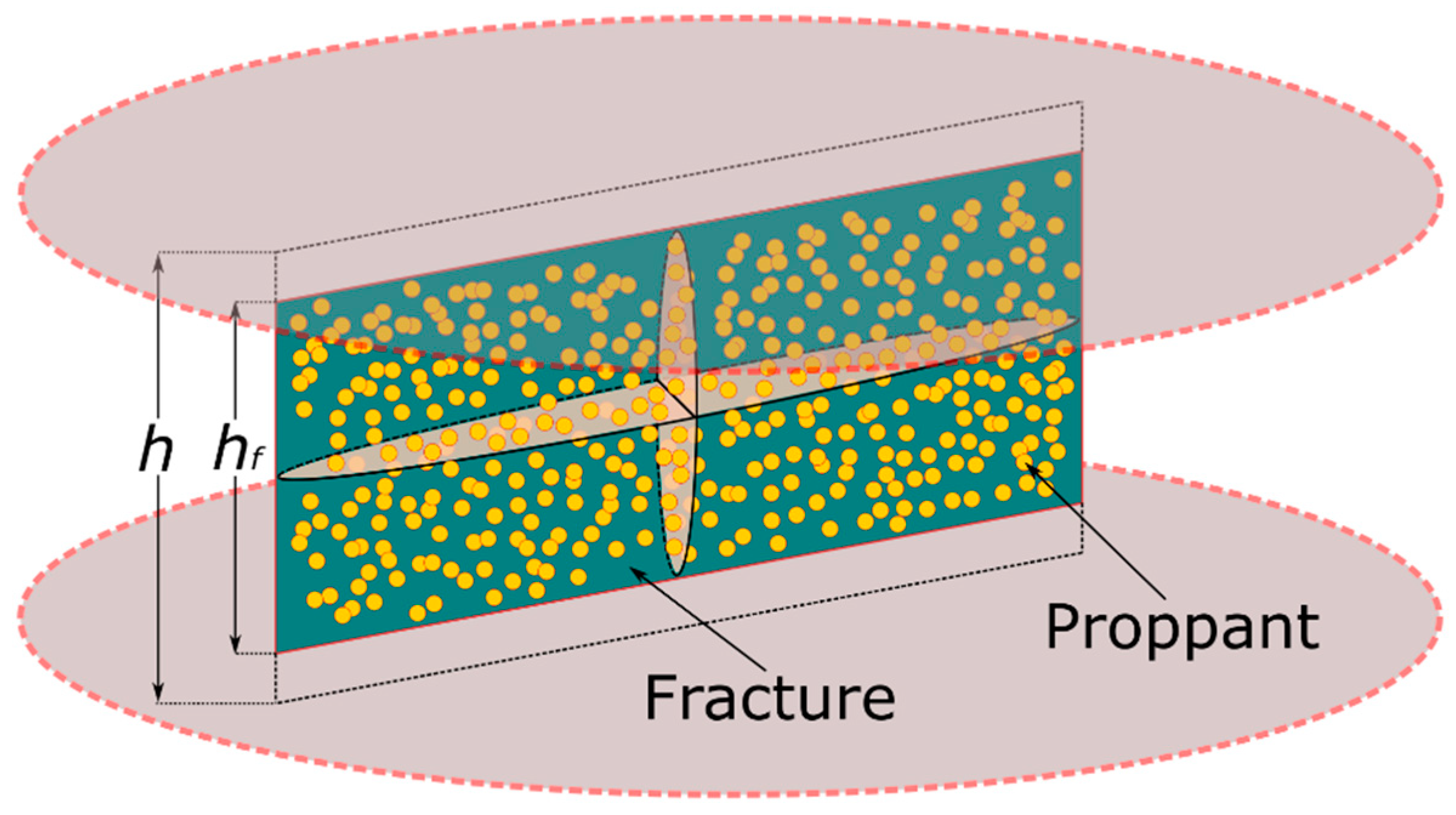
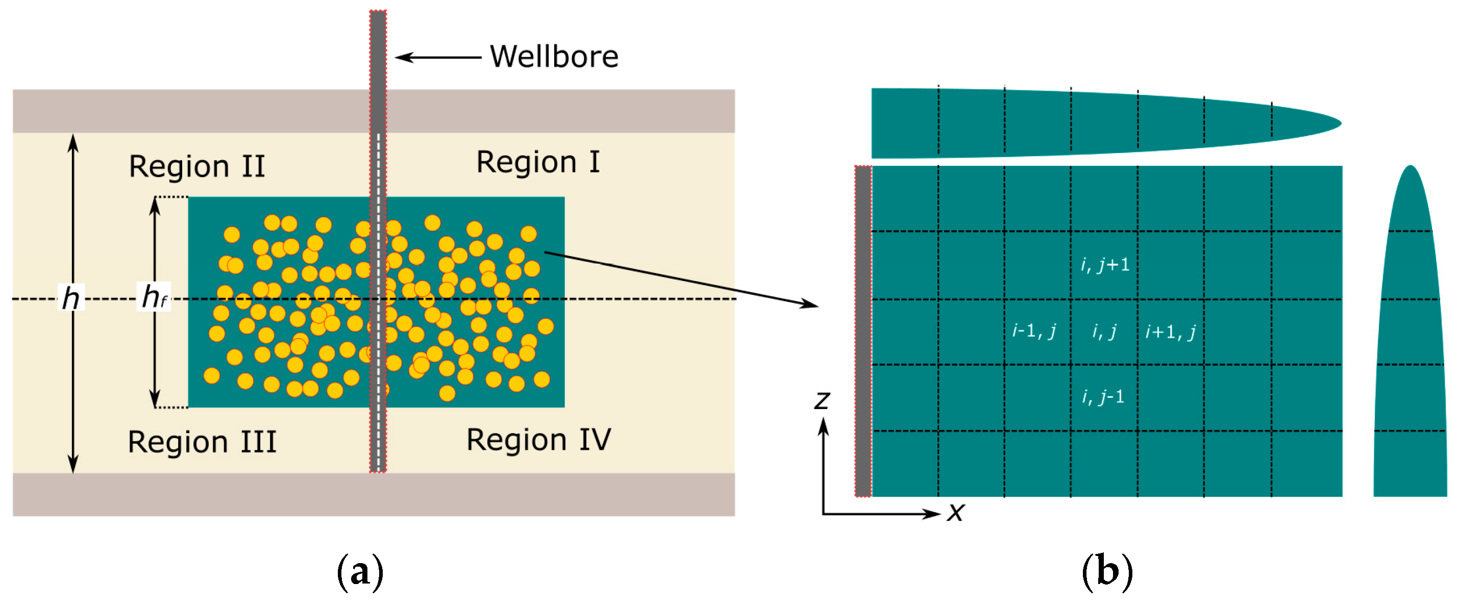
• The fracture is symmetrical with respect to the wellbore along the horizontal direction and located at the center of the reservoir along the vertical direction;
• The effect of leak-off is neglected;
• The fracture is vertical; and
• The fracture width will not change during the production, and the properties of the proppant-pack are uniform.

2.2. Fracture Propagation Model

In this work, the calculation procedures of the transient flow behavior of the nonuniform-width fractures contain two parts. The first part is predicting the geometry of the fracture propagation model with non-uniform widths, and the second part is calculating the pressure transient behavior of the nonuniform-width fractures. In the fracture propagation model, the pressure drawdown, which is caused by the fluid flow, is given as Nordgren [20]:

$$q=-{\beta }_1{\beta }_2\frac{\pi }{64}\frac{h_f{W}^3}{{\mu }_i}\frac{\partial \Delta p_f}{\partial x}$$

(1)

whereas the fracture width is a function of time and position, which can be expressed as Nordgren [18]:

$$W\left(x,t\right)=\frac{\left(1-v\right)h_f\Delta p_f\left(x,t\right)}{E}$$

(2)

Inserting Equation (2) into Equation (1) yields:

$$q=-{\beta }_1{\beta }_2\frac{\pi }{256}\frac{E}{\left(1-v\right){\mu }_i}\frac{\partial \left(W^4\right)}{\partial x}$$

(3)

Figure 2 shows the top view of the discretion of the fracture segments. Thus, the discretion form of Equation (3) at the mth time step can be written as:

$$q_{i+\raisebox{1ex}{$1$}\!\left/ \!\raisebox{-1ex}{$2$}\right.}=-{\beta }_1{\beta }_2\frac{\pi }{256}\frac{E}{\left(1-v\right){\mu }_i\Delta x}\left[{\left(W_{i+1}^m\right)}^4-{\left(W_i^m\right)}^4\right]$$

(4)

The mass balance equation that neglects the leak-off is given by Nordgren [18]:

$$\frac{\partial q}{\partial x}+\frac{\pi h_f}{4}\frac{\partial W}{\partial t}=0$$

(5)

Equation (5) can be discretized into:

$$\frac{\Delta t}{2}\frac{1}{\Delta x}\left(q_{i+\raisebox{1ex}{$1$}\!\left/ \!\raisebox{-1ex}{$2$}\right.}^{m+1}-q_{i-\raisebox{1ex}{$1$}\!\left/ \!\raisebox{-1ex}{$2$}\right.}^{m+1}+q_{i+\raisebox{1ex}{$1$}\!\left/ \!\raisebox{-1ex}{$2$}\right.}^m-q_{i-\raisebox{1ex}{$1$}\!\left/ \!\raisebox{-1ex}{$2$}\right.}^m\right)+\frac{\pi h_f}{4}\left(W_i^{m+1}-W_i^m\right)=0$$

(6)

Applying Equations (4) and (6) to the fracture segments, and solving the system of equations with the Newton–Raphson method, the fracture propagation can be readily predicted.

2.3. Formulation of Fracture Flow

Since we assume that the fracture is symmetrical corresponding to the wellbore and located at the center of the reservoir along the vertical direction, one-quarter of the fracture is sufficient to represent the entire fracture. In Figure 3a, we divided the fractured reservoir model into four regions, and the sub-fracture in Region I is investigated in this work. In Figure 3b, the sub-fracture in Region I is discretized into N_f small segments. According to the mass balance theory, the transient flow equation for the oil flow can be written as Ertekin et al. [21]:

$$\frac{{\partial }^2{p}_f}{\partial x^2}+\frac{{\partial }^2{p}_f}{\partial z^2}+\frac{B\mu q}{\beta \Delta x\Delta lw{k}_f}=\frac{\mu {\varphi }_f{c}_{tf}}{\beta k_f}\frac{\partial p_f}{\partial t}$$

(7)

Applying the finite difference approximation to Equation (7), the fracture flow equation for an arbitrary fracture segment (i, j) at the nth timestep can be expressed as:

$$\begin{array}{l}\frac{1}{\Delta x^2}\left[\left(p_{f,i+1,j}^n-p_{f,i,j}^n\right)-\left(p_{f,i,j}^n-p_{f,i-1,j}^n\right)\right]\\ +\frac{1}{\Delta z^2}\left[\left(p_{f,i,j+1}^n-p_{f,i,j}^n\right)-\left(p_{f,i,j}^n-p_{f,i,j-1}^n\right)\right]\\ -\frac{B\mu }{\beta \Delta x\Delta z{w}_f{k}_f}{q}_{f,i,j}^n=\frac{\mu {\varphi }_f{c}_{tf}}{\beta k_f\Delta t}\left(p_{f_{i,j}}^n-p_{f_{i,j}}^{n-1}\right)\end{array}$$

(8)

Rearranging Equation (8) has the following:

$$\begin{array}{l}{T}_{i+\raisebox{1ex}{$1$}\!\left/ \!\raisebox{-1ex}{$2$}\right.,j}\left(p_{f,i+1,j}^n-p_{f,i,j}^n\right)-T_{i-\raisebox{1ex}{$1$}\!\left/ \!\raisebox{-1ex}{$2$}\right.,j}\left(p_{f,i,j}^n-p_{f,i-1,j}^n\right)\\ +T_{i,j+\raisebox{1ex}{$1$}\!\left/ \!\raisebox{-1ex}{$2$}\right.}\left(p_{f,i,j+1}^n-p_{f,i,j}^n\right)-T_{i,j-\raisebox{1ex}{$1$}\!\left/ \!\raisebox{-1ex}{$2$}\right.}\left(p_{f,i,j}^n-p_{f,i,j-1}^n\right)\\ +q_{f,i,j}^n={\left(\frac{\Delta x\Delta z{w}_f{\varphi }_f{c}_{tf}}{B\Delta t}\right)}_{i,j}\left(p_{f,i,j}^n-p_{f,i,j}^{n-1}\right)\end{array}$$

(9)

where

$$\left\{\begin{array}{l}{T}_{i\pm \raisebox{1ex}{$1$}\!\left/ \!\raisebox{-1ex}{$2$}\right.,j}=2{\left[{\left(\frac{w_f\Delta z{\beta }_1{k}_f}{\mu B\Delta x}\right)}_{i,j}^{-1}+{\left(\frac{w_f\Delta z{\beta }_1{k}_f}{\mu B\Delta x}\right)}_{i\pm 1,j}^{-1}\right]}^{-1}\\ T_{i,j\pm \raisebox{1ex}{$1$}\!\left/ \!\raisebox{-1ex}{$2$}\right.}=2{\left[{\left(\frac{w_f\Delta x{\beta }_1{k}_f}{\mu B\Delta z}\right)}_{i,j}^{-1}+{\left(\frac{w_f\Delta x{\beta }_1{k}_f}{\mu B\Delta z}\right)}_{i,j\pm 1}^{-1}\right]}^{-1}\end{array}\right.$$

(10)

Applying Equation (9) to all the fracture segments in Region I will lead to N_f linear equations.

2.4. Formulation of Matrix Flow

According to the Newman product method, the pressure change at the nth timestep at fracture segment (i, j) that is caused by a flux that occurs at the kth timestep at fracture segment (I, J) can be expressed as an integration of the product of three source functions. These three source functions include an instantaneous plane source function along the x-direction in an unbounded reservoir, an instantaneous line source function along the y-direction in an unbounded reservoir, and an instantaneous plane source function along the z-direction in a bounded reservoir [6]. Thus, the pressure change can be calculated with

$$\begin{array}{l}\frac{1}{q_{f,I,J}^k}\Delta p_{f,i,j}^n=\frac{1}{{\varphi }_m{c}_{tm}\Delta x_{I,J}\Delta z_{I,J}}{\displaystyle {\int }_{t^{k-1}}^{t^k}}\\ \frac{1}{2}\left\{\mathrm{erf}\left[\frac{0.5\Delta x_{I,J}+\left(x_{i,j}-x_{I,J}\right)}{\sqrt{4{\eta }_m\left(t^n-\tau \right)}}\right]+\mathrm{erf}\left[\frac{0.5\Delta x_{I,J}-\left(x_{i,j}-x_{I,J}\right)}{\sqrt{4{\eta }_m\left(t^n-\tau \right)}}\right]\right\}\tau \\ \cdot \exp \left[-\frac{{\left(y_{i,j}-y_{I,J}\right)}^2}{4{\eta }_m\left(t^n-\tau \right)}\right]/\sqrt{4\pi {\eta }_m\left(t^n-\tau \right)}\\ \cdot \frac{\Delta z_{I,J}}{z_e}\left\{1+\frac{4z_e}{\pi \Delta z_{I,J}}{\displaystyle \sum _{m=1}^{\infty }\frac{1}{m}\exp \left[-\frac{m^2{\pi }^2{\eta }_m\left(t^n-\tau \right)}{h^2}\right]\sin \frac{m\pi \Delta z_{I,J}}{2h}\cos \frac{m\pi z_{I,J}}{h}\cos \frac{m\pi z_{i,j}}{h}}\right\}\mathrm{d}\tau \end{array}$$

(11)

A detailed introduction of the derivation of Equation (11) can be found in Teng et al. [19]. For the sake of convenience, Equation (11) is rewritten as:

$$\Delta p_{f,i,j}^n=q_{f,I,J}^k{G}_{I,J}^{n,k}\left(i,j\right)$$

(12)

where the G term in Equation (12) denotes the term on the right-hand side of Equation (11). On the basis of the superposition principle, the total pressure change at the nth timestep at fracture segment (i, j) can be calculated by summing up the pressure changes that are induced by all the fracture segments from the 1st timestep to the nth timestep, which can be expressed as:

$$\Delta p_{f,i,j}^n={\displaystyle \sum _{k=1}^{k=n}{q}_{f,I,J}^k\left[\begin{array}{c}{\displaystyle \sum _{{\Omega }_{\mathrm{I}}}{G}_{I,J}^{n,k}\left(i,j\right)}+{\displaystyle \sum _{{\Omega }_{\mathrm{II}}}{G}_{-I,J}^{n,k}\left(i,j\right)}\\ +{\displaystyle \sum _{{\Omega }_{\mathrm{III}}}{G}_{-I,-J}^{n,k}\left(i,j\right)}+{\displaystyle \sum _{{\Omega }_{\mathrm{IV}}}{G}_{I,-J}^{n,k}\left(i,j\right)}\end{array}\right]}$$

(13)

where the fracture segment (−I, J), (−I, −J), and (I, −J) present the counterpart of fracture segment (I, J) in Region II, Region III, and Region IV, respectively. Equation (13) is a linear equation. Applying Equation (13) to all the fracture segments in Region I will result in N_f linear equations.

2.5. Formulation of Wellbore

Along the vertical direction, for one-quarter of the nonuniform-width fractures, there are n_w fracture segments that are connected to the wellbore. For an arbitrary fracture segment that is connected to the wellbore, the fluid flow can be described with Darcy’s law:

$$q_{f-w,i,j}^n=\frac{{\beta }_1{k}_f{w}_{f,i,j}\Delta z_{i,j}}{B\mu }\frac{p_{f,i,j}^n-p_w^n}{0.5\Delta x_{i,j}}$$

(14)

The total production can be calculated with:

$$q_w^n=4{\displaystyle {\sum }_1^{n_w}{q}_{f-w,i,j}^n}$$

(15)

Applying Equation (14) to the n_w fracture segment that are connected to the wellbore and Equation (15) to the wellbore, we will have n_w + 1 linear equations. Thus, by combining the matrix flow equations, fracture flow equations, and wellbore equations, we will have 2N_f + n_w + 1 linear equations. In addition, we have 2N_f + n_w + 1 unknowns, including N_f fracture pressure p_f, N_f matrix-fracture flux rate q_f, n_w fracture-wellbore flux rate q_f-w, and 1 well production rate q_w for constant bottomhole pressure condition (or 1 bottomhole pressure p_w for constant production rate condition). Thus, the system of the linear equation can be readily solved with the Gaussian Elimination method.

3. Validation

The proposed semi-analytical model is validated against commercial software (Eclipse 2006). The values of the parameters that are used in the model are as follows: k_m = 0.01 md, x_f/2 = 25 m, c_tm = 0.012 MPa⁻¹, c_tf = 0.012 MPa⁻¹, μ = 1 mPa∙s, ϕ_m = 0.2, ϕ_f = 0.2, p_i = 30 MPa, h = 30 m, h_f = 25 m, the production length is 10,000 days, and the dimension of the reservoir model is 1010 × 1010 × 30 m³, which is sufficiently large to avoid the boundary effect. The validation is conducted under the constant production rate condition of q_w = 1 m³/day. Figure 4 shows a local side view of the permeability distribution of the nonuniform-width fractures used in the Eclipse. The local refined grid technique is applied to characterize the fracture. In order to make the fracture conductivity distribution of the model in Eclipse consistent with that of the model in the semi-analytical model, we remain the fracture width unchanged and vary the fracture permeability through the fracture in Eclipse, while maintaining the fracture permeability unchanged and vary the fracture width through the fracture in the semi-analytical model. Figure 5 compares the pressure drop plot and pressure derivative plot from the proposed model to those from Eclipse. As shown in Figure 5, the results from the proposed model present excellent agreements to those from Eclipse, implying that the proposed model is reliable to characterize the transient flow behavior of the nonuniform-width fractures. It is worth noting that, although the numerical software can simulate the nonuniform-width fracture, the proposed model has obvious advantages in computational efficiency.

4. Results and Discussion

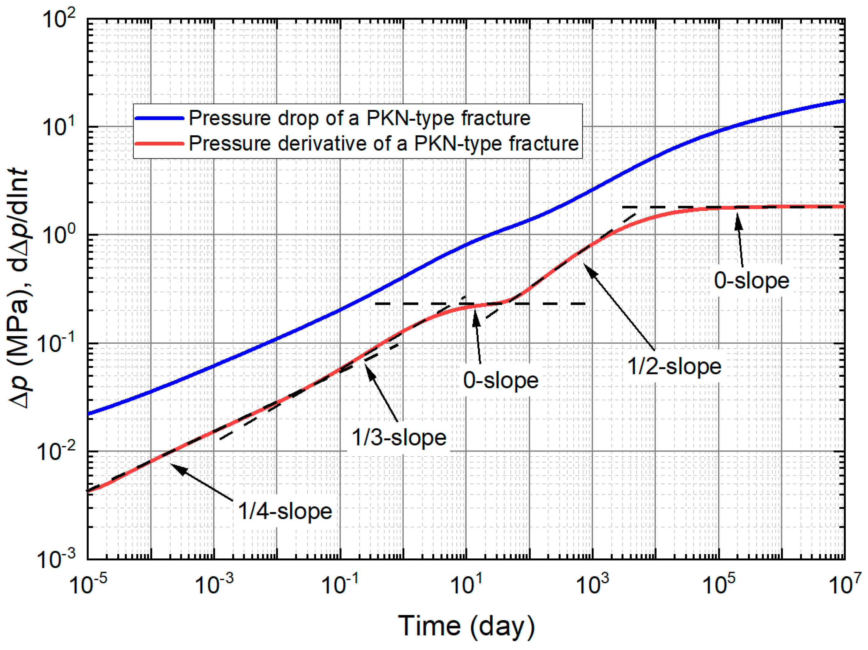
Combining the proposed semi-analytical model with the PKN fracture model, we carried out a comprehensive study of the pressure transient behavior of the nonuniform-width fractures. In this work, the benchmark values of the parameters that are used in this work are listed in

Table 1. Benchmark values of the parameters that are used in this work.

Parameter	Value	Parameter	Value
qi	4.32 × 103 m3/day	Qi	4.32 × 105 m3
μi	100 mPa∙s	hf	40 m
E	4.5 × 104 MPa	v	0.2
ti	6.94 × 10−3 day	h	50 m
μo	1 mPa∙s	kf	1 × 106 md
km	1 × 10−2 md	ctm	1.12 × 10−3 MPa−1
ctf	1.12 × 10−3 MPa−1	ϕm	0.2
ϕf	0.2	pw	5 MPa

. The reason the benchmark parameters are different from the validated parameters is because the smaller size fracture built in the numerical software can improve computational efficiency.

4.1. Flow Regimes

In order to recognize the flow regimes that can be observed during the production of a PKN-type fracture, the transient flow behavior of the fractured well is investigated under the constant flow rate condition, such that the flow regimes can be diagnosed by identifying the slopes of the pressure derivative plot. Figure 6 presents the pressure drop plot together with the pressure derivative plot of the benchmark PKN-type fracture. It can be found in this figure that at the early production period, there is a 1/4-slope region on the plot, which denotes bilinear flow [22]. As the production proceeds, a 1/2-slope region, which indicates the formation of linear flow [22], appears on the pressure derivative plot. At the late production period, the 0-slope region implies the appearance of horizontal pseudo-radial flow. Figure 7a–c show the top view of the schematics of the bilinear flow, formation linear flow, and horizontal pseudo-radial flow, respectively.

Furthermore, the flow regimes of the PKN-type fracture are investigated with a smaller fracture height (h_f = 10 m) and less injection volume (Q_i = 1.08 × 10⁵ m³). Figure 8 shows the pressure transient plots of the new fracture model. In Figure 8, it can be found that in addition to the bilinear flow, formation linear flow, and horizontal pseudo-radial flow, two more flow regimes can be observed on the pressure derivative plot. The 1/3-slope region in Figure 8 indicates elliptical flow and the first 0-slope region indicates vertical pseudo-radial flow. Figure 9 shows a side view of the schematic of the elliptical flow and the vertical pseudo-radial flow. As shown in Figure 9, since the new fracture model has a much lower fracture height (h_f = 10 m) than the reservoir thickness (h = 50 m), the fluid flow along the vertical direction exerts a significant influence on the flow regimes. Therefore, one can observe the regimes of elliptical flow and pseudo-radial flow along the vertical direction in Figure 8.

4.2. Sensitivity Analysis

In this section, the authors carried out a comprehensive study of the effects of fracture height, injection rates, and Young’s modulus on the well performance. The transient flow behavior of the PKN-type fractures is studied with the constant bottomhole pressure condition.

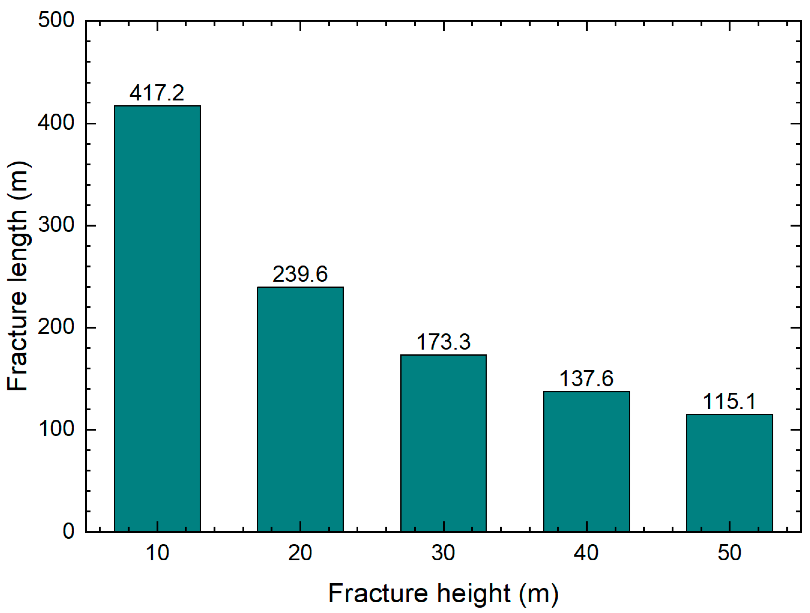
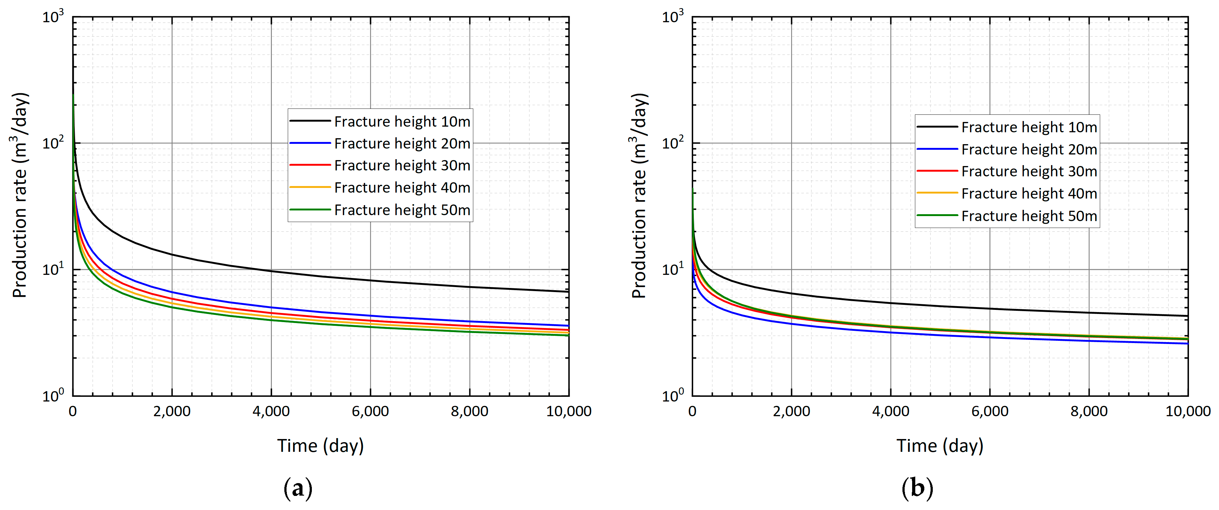
4.3. Fracture Height

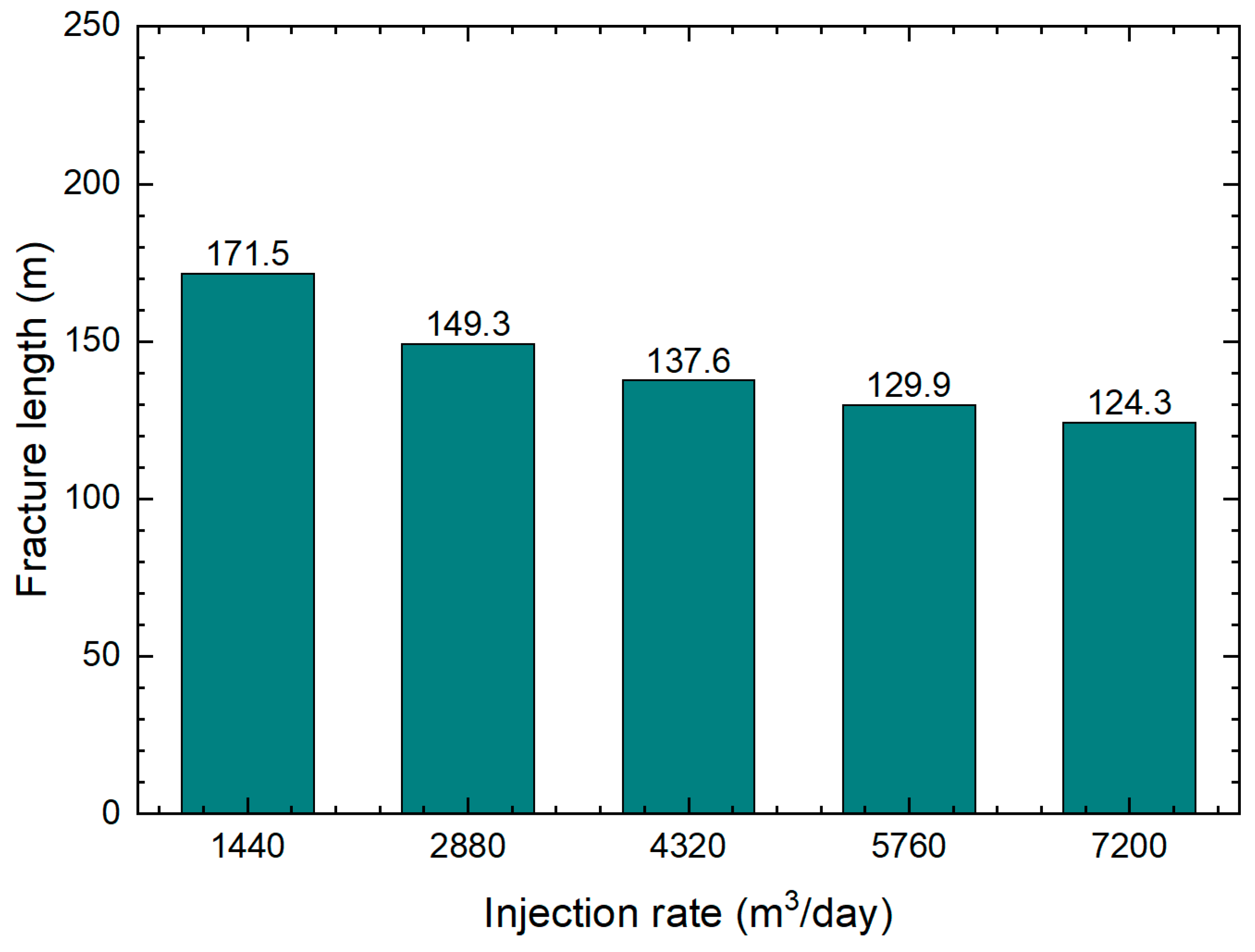
The fracture height is varied from 10 m to 50 m in order to explore the effect of fracture height on the propagation and well performance of the PKN-type fractures. Figure 10 shows the fracture lengths that are calculated with the PKN model. It is shown in this figure that as the fracture height is increased, the fracture length is decreased. This is because the geometries of the PKN-type fracture are calculated with the same injection volume. In addition, it can be observed that the decrease in fracture length can be more significant if the change in fracture height occurs at a smaller value. For example, as the fracture height is increased from 10 m to 20 m, the fracture length is decreased from 417.2 m to 239.6 m, whereas as the fracture height is increased from 40 m to 50 m, the fracture length is decreased only from 137.6 m to 115.1 m.

Figure 11 illustrates the width distribution of one-quarter of the PKN-type fractures that are calculated with different fracture heights. It is worth noting that the axes in the sub-figures indicate dimensionless length and height. The coordinate of x/x_f/2 = 0 indicates the position of the wellbore, and the position of (x/x_f/2 = 0, z/h_f/2 = 0) indicates the center of the fracture. In Figure 11a–e, the widest part of the fracture can be found at the center of the PKN-type fractures, while the narrowest part appears at the edge of the fractures. Comparing the fracture width distribution of the sub-figures, it can be readily found that a larger fracture height can induce a lower fracture width distribution.

Figure 12a,b compares the well production rate with different fracture heights of k_f = 1 × 10⁵ md and k_f = 1 × 10³ md, respectively. In Figure 12a, it is shown that the well production rate is decreased as the fracture height is increased. It is noted that a smaller fracture height leads to a larger fracture length (see Figure 10), thereby the oil from further well area can be extracted. Thus, a larger fracture length can be more favorable for improving the well productivity for larger fracture permeability. For a small fracture permeability (e.g., k_f = 1 × 10³ md in Figure 12b), one can find that the highest well production rate happens at the fracture height of 10 m, while the lowest happens at the fracture height of 20 m. The fracture heights of 30 m through 50 m lead to intermediate well productivity. This implies that for the scenarios of low fracture permeability, the fracture height, together with the fracture length, both play important roles in influencing the well productivity.

4.4. Injection Rate

Figure 13 illustrates the fracture length of the PKN-type fracture that is calculated with the same injection volume (i.e., Q_i = 1.08 × 10⁵ m³) while different injection rates (i.e., 1.44 × 10³ m³/day, 2.88 × 10³ m³/day, 4.32 × 10³ m³/day, 5.76 × 10³ m³/day, and 7.20 × 10³ m³/day). One can find that a higher injection rate will result in a smaller fracture length. Figure 14 shows the fracture width distribution of the PKN-type fractures with different injection rates. It is observed in Figure 14 that as the injecting rate is increased, the fracture width is decreased. The calculated results shown in Figure 13 and Figure 14 can be explained as follows: a lower injecting rate implies a smaller fluid pressure within the fracture, which will lead to a higher fracture closure stress. A higher closure stress will render the fracture open less but propagate further into the reservoir. Therefore, a lower injection rate will induce narrower but longer fractures.

Figure 15 compares the fracture production rate of the PKN-type fractures with different injection rates of k_f = 1 × 10⁵ md and k_f = 1 × 10³ md. As shown in Figure 15a, the fractured well exhibits a smaller well production rate with a higher injection rate of k_f = 1 × 10⁵ md. This is because the fracture has a smaller length with higher injection, and a smaller fracture length can induce lower well productivity for high fracture permeability (i.e., k_f = 1 × 10⁵ md). Figure 15b shows that the fracture productivity undergoes a small difference with k_f = 1 × 10³ md. Comparing the calculated results presented in Figure 13, Figure 14 and Figure 15 to those shown in Figure 10, Figure 11 and Figure 12, one can see that the effect of injection rate on the fracture length and well productivity is less noticeable than the effect of fracture height.

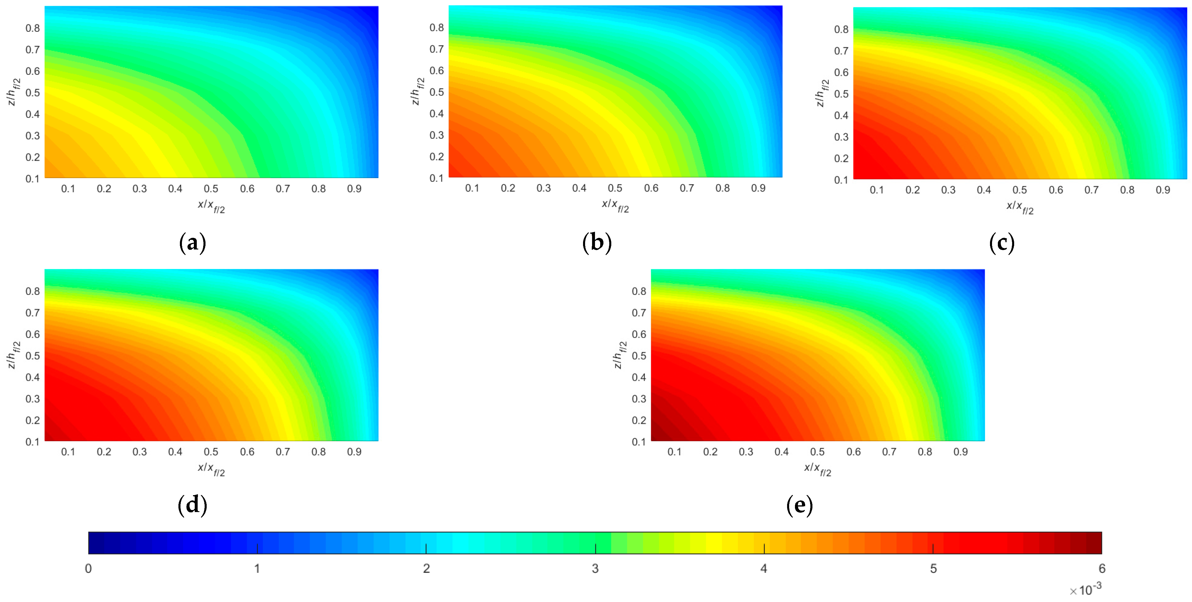
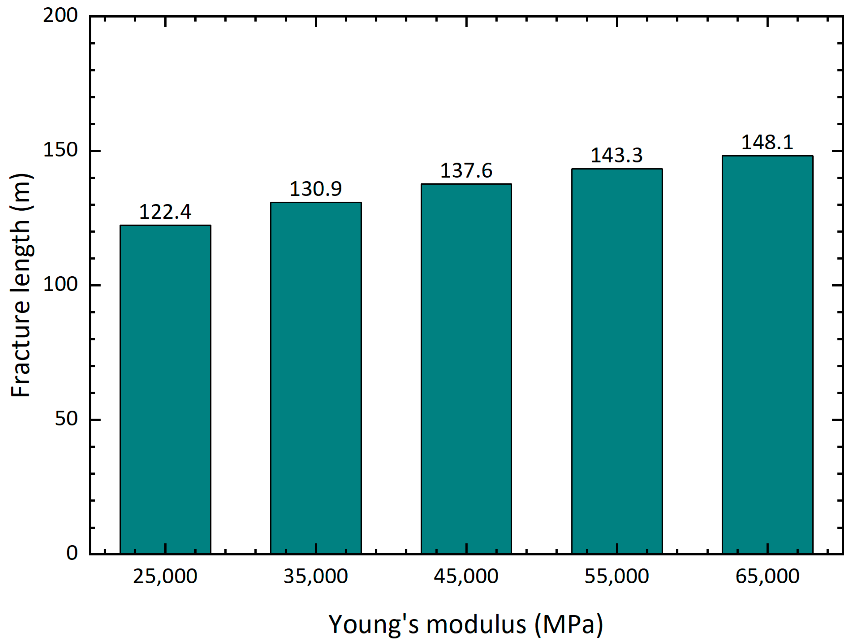
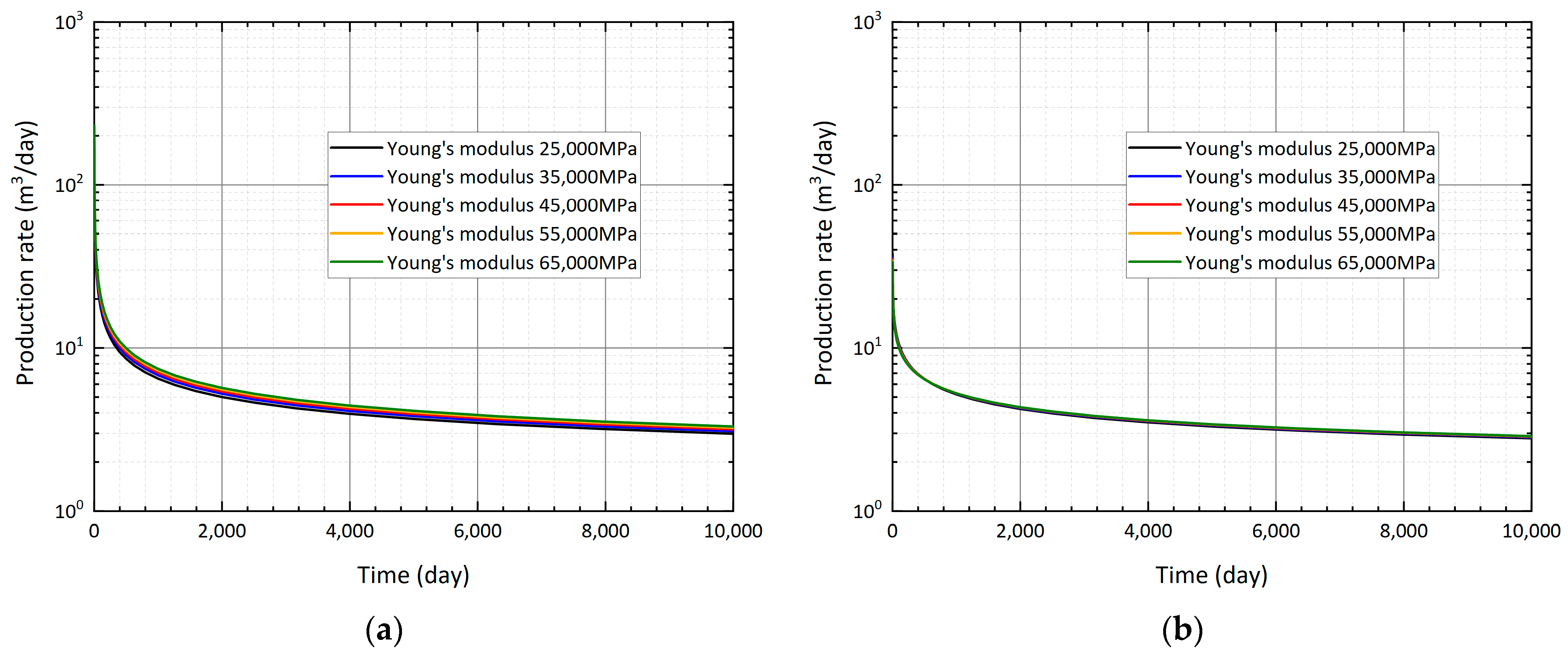
4.5. Young’s Modulus

The Young’s modulus varies from 2.5 × 10⁴ MPa to 6.5 × 10⁴ Mpa in order to study its effect on fracture geometry and well performance. Figure 16 exhibits the fracture lengths that are calculated with different Young’s moduli. As shown in this figure, the fracture length is positively correlated with Young’s modulus. Figure 17 presents the fracture width distribution of the PKN-type fracture with different Young’s moduli. It is observed that a larger Young’s modulus results in narrower fractures. This is because Young’s modulus represents the stiffness of the rock matrix. A larger Young’s modulus indicates that the rock matrix is more difficult to deform. Thus, the hydraulic fracture has a smaller width with a larger Young’s modulus. Since the injecting volume remains unchanged, a larger fracture width will result in a narrower fracture.

Figure 18 demonstrates the production rate of the PKN-type fractures with different Young’s moduli of k_f = 1 × 10⁵ md and k_f = 1 × 10³ md. In Figure 18a, the fracture production rate is higher with smaller Young’s modulus. This is because the fracture length plays a more significant role in influencing the well productivity. Hence, for the scenario of the largest Young’s modulus (i.e., E = 6.5 × 10⁴ MPa), which has the longest fracture, the well production rate presents the highest value through the production. In Figure 18b, the well performance shows a negligible difference with different Young’s moduli, implying that Young’s modulus exerts a slight influence on the well performance with small fracture permeability (e.g., k_f = 1 × 10³ md).

5. Conclusions

In this work, the authors conducted a comprehensive study of the transient flow behavior of the nonuniform-width fractures. The contributions of this work can be summarized into two aspects: first, the author proposed a semi-analytical model in a three-dimension to consider the fluid flow along the vertical direction around the PKN-type fractures; second, the proposed semi-analytical model is combined with the PKN fracture propagation model to investigate the effects of fracturing treatments and rock matrix properties on the well performance. On the basis of the calculated results, the following conclusions can be formed:

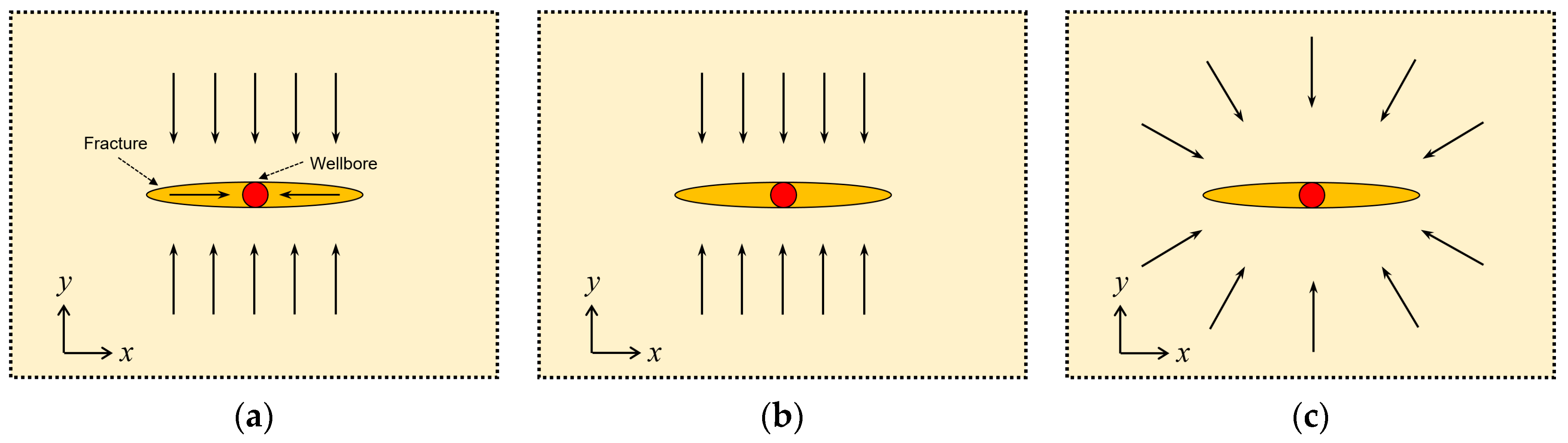
• If a PKN-type fracture has a sufficiently large height, one can observe the bilinear flow, formation linear flow, and horizontal pseudo-radial flow during the production. If the fracture height is sufficiently small compared to the formation thickness, the vertical flow around the fracture cannot be neglected, and one can observe the vertical elliptical flow and vertical pseudo-radial flow during the production;
• With the same injection volume, a larger fracture height can induce a shorter fracture length. For the scenarios of high fracture permeability (e.g., k_f = 1 × 10⁵ md), a longer but lower-height fracture can be more favorable for improving the well productivity;
• A lower injecting rate can render the PKN-type fracture penetrate further into the reservoir, leading to a higher well productivity of the high-permeability fractures. If the fracture permeability is sufficiently small, the injecting rate can only slightly influence the well performance.
• A larger value of Young’s modulus can result in a longer but narrower PKN-type fracture as well as a higher well productivity for high-permeability fractures. The influence of Young’s modulus on the well performance is negligible for the scenarios of low fracture permeability.
• In comparison to the fracture height, the injection rate and Young’s modulus exert a smaller influence on the fracture growth and well productivity.

References

1. Holditch, S.A.; Holcomb, D.L.; Rahim, Z. Using Tracers to Evaluate Propped Fracture Width. In Proceedings of the SPE 26922 Presented at SPE Eastern Regional Meeting, Pittsburgh, PA, USA, 2–4 November 1993. [Google Scholar]
2. Wright, E.A.; Davis, E.J.; Golich, G.M.; Ward, J.F.; Demetrius, S.L.; Minner, W.A.; Weijers, L. Downhole Tiltmeter Fracture Mapping: Finally Measuring Hydraulic Fracture Dimensions. In Proceedings of the SPE 46194 Presented at SPE Western Regional Meeting, Bakersfield, CA, USA, 10–13 May 1998. [Google Scholar]
3. van Dam, D.B.; Papanastasiou, P.; de Pater, C.J. Impact of Rock Plasticity on Hydraulic Fracture Propagation and Closure. In Proceedings of the SPE 63172 Presented at SPE Annual Technical Conference and Exhibition, Dallas, TX, USA, 1–4 October 2000. [Google Scholar]
4. Geertsma, J. Two-dimensional Fracture-propagation Models. Soc. Pet. Eng. AIME J. 1989, 12, 81–94. [Google Scholar]
5. Geertsma, J.; Haafkens, R. Comparison of the theories for predicting width and extent of vertical hydraulically induced fractures. J. Energy Resour. Technol. 1979, 101, 8–19. [Google Scholar] [CrossRef]
6. Gringarten, A.C.; Ramey, H.J. The Use of Source and Green’s Functions in Solving Unsteady-Flow Problems in Reservoirs. SPE J. 1973, 13, 285–296. [Google Scholar] [CrossRef]
7. Gringarten, A.C.; Ramey, H.J. Unsteady-State Pressure Distributions Created by a Well with a Single Infinite-Conductivity Vertical Fracture. SPE J. 1974, 14, 347–360. [Google Scholar] [CrossRef]
8. Gringarten, A.C.; Ramey, H.J. Unsteady-State Pressure Distributions Created by a Well with a Single Horizontal Fracture, Partial Penetration, or Restricted Entry. SPE J. 1974, 14, 413–426. [Google Scholar] [CrossRef]
9. Rodriguez, F.; Horne, R.N.; Cinco-Ley, H. Partially Penetrating Vertical Fractures: Pressure Transient Behavior of a Finite-Conductivity Fracture. In Proceedings of the SPE 13057 Presented at SPE Annual Technical Conference and Exhibition, Houston, TX, USA, 16–19 September 1984. [Google Scholar]
10. Zhou, W.; Banerjee, R.; Poe, B.D.; Spath, J. Semianalytical Production Simulation of Complex Hydraulic-Fracture-Networks. SPE J. 2014, 19, 6–18. [Google Scholar] [CrossRef]
11. Yang, D.; Zhang, F.; Styles, J.A.; Gao, J. Performance Evaluation of a Horizontal Well with Multiple Fractures by Use of a Slab-Source Function. SPE J. 2015, 20, 652–662. [Google Scholar] [CrossRef]
12. Luo, W.; Tang, C. Pressure-Transient Analysis of Multiwing Fractures Connected to a Vertical Wellbore. SPE J. 2015, 20, 360–367. [Google Scholar]
13. Chen, Z.; Liao, X.; Zhao, X.; Lv, S.; Zhu, L. A Semianalytical Approach for Obtaining Type Curves of Multiple-Fractured Horizontal Wells with Secondary-Fracture Networks. SPE J. 2016, 21, 538–549. [Google Scholar] [CrossRef]
14. Jia, P.; Cheng, L.; Clarkson, C.R.; Qanbari, F.; Huang, S.; Cao, R. A Laplace-Domain Hybrid Model for Representing Flow Behavior of Multifractured Horizontal Wells Communicating through Secondary Fractures in Unconventional Reservoirs. SPE J. 2017, 22, 1856–1876. [Google Scholar] [CrossRef]
15. Xiao, C.; Dai, Y.; Tian, L.; Lin, H.; Zhang, Y.; Yang, Y.; Hou, T.; Deng, Y. A Semianalytical Methodology for Pressure-Transient Analysis of Multiwell-Pad-Production Scheme in Shale Gas Reservoirs, Part 1: New Insights into Flow Regimes and Multiwell Interference. SPE J. 2017, 23, 885–905. [Google Scholar] [CrossRef]
16. Teng, B.; Li, H.; Yu, H. A Novel Analytical Fracture-Permeability Model Dependent on Both Fracture Width and Proppant-Pack Properties. SPE J. 2020, 25, 3031–3050. [Google Scholar] [CrossRef]
17. Yu, W.; Wu, K.; Sepehrnoori, K. A Semianalytical Model for Production Simulation from Nonplanar Hydraulic-Fracture Geometry in Tight Oil Reservoirs. SPE J. 2016, 21, 1028–1040. [Google Scholar] [CrossRef]
18. Barton, N.; Bandis, S.; Bakhtar, K. Strength, deformation and conductivity coupling of rock joints. Int. J. Rock Mech. Min. Sci. 1985, 22, 121–140. [Google Scholar] [CrossRef]
19. Teng, B.; Li, H.A. A Semi-Analytical Model for Characterizing the Pressure Transient Behavior of Finite-Conductivity Horizontal Fractures. Transp. Porous Med. 2018, 123, 367–402. [Google Scholar] [CrossRef]
20. Nordgren, R.P. Propagation of a Vertical Hydraulic Fracture. SPE J. 1972, 12, 306–314. [Google Scholar] [CrossRef]
21. Ertekin, T.; Abou-Kassem, J.H.; King, G.R. Basic Applied Reservoir Simulation; SPE Textbook Series; Society of Petroleum Engineers: Richardson, TX, USA, 2001. [Google Scholar]
22. Cinco-Ley, H.; Samaniego-V, F. Transient Pressure Analysis for Fractured Wells. SPE J. 1981, 33, 1749–1766. [Google Scholar] [CrossRef]
Figure 1. Schematic of a partially penetrating fracture with nonuniform width.
Energies 16 07920 g001
Figure 2. Discretization of the fracture segments.
Energies 16 07920 g002
Figure 3. The model used in this work: (a) division of the fractured reservoir model; and (b) discretion of one-quarter of the fracture.
Energies 16 07920 g003
Figure 4. Permeability distribution of the nonuniform-width fractures used in Eclipse (md).
Energies 16 07920 g004
Figure 5. Comparison between the results from the proposed model and those from Eclipse.
Energies 16 07920 g005
Figure 6. Pressure transient plot of the benchmark PKN-type fracture.
Energies 16 07920 g006
Figure 7. Top view of the schematics of (a) bilinear flow, (b) formation linear flow, and (c) horizontal pseudo-radial flow.
Energies 16 07920 g007
Figure 8. Pressure transient plot of the PKN-type fracture with fracture height of 10 m.
Energies 16 07920 g008
Figure 9. Side view of the schematics of (a) elliptical flow and (b) vertical pseudo-radial flow.
Energies 16 07920 g009
Figure 10. Fracture length of the PKN-type fractures as a function of fracture height.
Energies 16 07920 g010
Figure 11. Fracture width distribution of the PKN-type fractures with different fracture heights: (a) hf = 10 m; (b) hf = 20 m; (c) hf = 30 m; (d) hf = 40 m; and (e) hf = 50 m.
Energies 16 07920 g011
Figure 12. Production rate of the PKN-type fracture with different fracture heights of (a) kf = 1 × 10⁵ md and (b) kf = 1 × 10³ md.
Energies 16 07920 g012
Figure 13. Fracture length of the PKN-type fractures as a function of injection rate.
Energies 16 07920 g013
Figure 14. Fracture width distribution of the PKN-type fractures with different injection rates: (a) qi = 1.44 × 10³ m3/day; (b) qi = 2.88 × 10³ m3/day; (c) qi = 4.32 × 10³ m3/day; (d) qi = 5.76 × 10³ m3/day; and (e) qi = 7.20 × 10³ m3/day.
Energies 16 07920 g014
Figure 15. Production rate of the PKN-type fracture with different injection rates of (a) kf = 1 × 10⁵ md and (b) kf = 1 × 10³ md.
Energies 16 07920 g015
Figure 16. Fracture length of the PKN-type fractures as a function of Young’s modulus.
Energies 16 07920 g016
Figure 17. Fracture width distribution of the PKN-type fractures with different Young’s moduli: (a) E = 2.5 × 10⁴ MPa; (b) E = 3.5 × 10⁴ MPa; (c) E = 4.5 × 10⁴ MPa; (d) E = 5.5 × 10⁴ MPa; (e) E = 6.5 × 10⁴ MPa.
Energies 16 07920 g017
Figure 18. Production rate of the PKN-type fracture with different Young’s moduli of (a) kf = 1 × 10⁵ md and (b) kf = 1 × 10³ md.
Energies 16 07920 g018