Thorough Analysis of the Reliability of Measurements on Chassis Roller Dynamometer and Accurate Energy Consumption Estimation for Electric Vehicles

Abstract

The energy consumption of the electric test vehicle on the roller dynamometer test bench is thoroughly investigated in this work. Initially, we extensively examined the relevant testing approaches on chassis dynamometer test benches. Then, we presented the main issues and limitations of this type of testing facility. After that, an experimental analysis was performed by recording the NEDC and the WLTP-class 2 standard driving cycle test data. It was found that the power consumption associated with specific test maneuvers could be accurately simulated via the roller dynamometer system. However, the experimental test results showed some disparities compared to the expected results from the simulation models. These findings supported identifying the dynamic behavior resulting from the tire and roller contact. The LuGre friction model provided the solution, incorporating friction-related physical models such as stick-slip and the Stribeck effect. In addition, adjustments were made to the LuGre model to consider the dynamic influences of the roller on the tire. Finally, we created a systematic estimation model for energy consumption by integrating the boundary conditions of the test bench, a generic model for energy estimation of electric vehicles, and the proposed tire–roller contact model. The overall model requires only the measured traction speed of the test vehicle and the auxiliary energy losses as physical inputs. The results proved that the proposed model enabled the estimation of the total power consumption with high accuracy.

1. Introduction

Chassis dynamometers are widely used in test environments in vehicle development due to their relatively simple configurations and versatility [1,2]. Their scope involves vehicles, from motorcycles to heavy industrial machinery. Roller test benches can be easily integrated into diverse research and development applications. They play a chief role in developing the advanced functionalities of modern mobility. A typical use for a chassis dynamometer will be to assign a standard driving cycle as a reference speed profile with time, a WLTP cycle, for instance. The reference driving cycle could be performed either by a real driver or a driving robot. Then, the performance of the test vehicle is evaluated after it undergoes the designated driving cycle. The loading machines of the chassis dynamometer generate movement according to a driving resistance curve corresponding to the wheels’ rotational speeds. The driving resistance curve is commonly identified as an n-order polynomial whose coefficients are determined via regression methods on the results of several experiments [3].

The classical road load simulation (RLS) is calculated with only three constant parameters, A, B, and C, attained from the test vehicle’s coast-down test [4,5,6,7]. Furthermore, the influences of road inclination, route curvature, acceleration dynamics, and ambient conditions, such as temperature and pressure, can be considered. After obtaining these parameters, a driving resistance force as a speed function is formulated. Thus, standard driving cycles like NEDC and WLTP can be performed using this technique. Moreover, it could be employed for evaluating the development goals [4,5,7].

It was emphasized that testing on a chassis dynamometer requires additional corrections to make the results more relevant to the corresponding road driving tests. The chassis dynamometer itself, however, creates an “environment” that adversely influences the experimental results. Depending on the focus of the investigations in a test bench facility, there is usually a conflict of objectives. A study was made in [8] to investigate the influence of altering some test conditions of a chassis dynamometer on fuel consumption. In the chassis dynamometer setup, some factors significantly influenced the fuel consumption measurement, such as pedal operating, speed error, vehicle alignment, tire type, tire pressure, and the simulated vehicle mass. Another issue is the conflict between acoustics experiments and controlling the climatic conditions of the chassis dynamometer test bench. The test concept for acoustic examinations of the test vehicle requires minimizing the noise from the test bench [9]. According to [9], heating and distortion effects may damage tires used even for a short time on rolling roads. As a solution, some dynamometer systems could be equipped with tire-cooling systems to reduce tire damage, as investigated by [10]. Nevertheless, an extensive air conditioning system would significantly impact acoustics [9]. It was shown in [11] that even different retaining methods affect the acoustic signature and the noise level of the test vehicle to various extents.

It is understood that tire contact with the roller is an important matter when representing the vehicle’s dynamic behavior. Hence, it is highly relevant for vehicle dynamic simulation models. Therefore, the tire contact on the bench must be thoroughly analyzed for chassis benches [11]. The tires of the drive wheels are placed on the rollers and are engaged with the rollers by means of friction forces. Therefore, in terms of constraints and potential sources of error, the chassis dynamometer directly influences the measurement results. These mainly concern the measurement of losses in the drive train and tires, as the rolling resistance of the tire mounted on the roller differs significantly from its actual value on the flat road. Furthermore, there is a noticeable difference between running it on rollers of different diameters [9]. The rollers’ size significantly affects the rolling resistance [12]. Moreover, in the same study, other influential aspects on the rolling were also investigated for each roller size: vertical load, angular speed, and inflation pressure. The results showed that the smaller the roller sides, the more sensitive the rolling resistance would be to changing other factors.

An approach for adjusting the driving resistances model of the chassis dynamometer is proposed in [6]. The authors introduced some adjustment factors to reproduce the chassis dynamometer’s driving resistances correctly. The procedure begins with data acquisition from on-road testing. Next, an offline simulation verifies the vehicle model by comparing the coast-down test results of actual and simulated values. Finally, an online simulation is executed on the test bench. The scaling factors for the rolling resistance model are tuned via a compensation model in the final stage. The adjustment factors were verified by comparing the results of the coast-down tests between the real-world measurements, simulation results, and test bench measurements. The accuracy of the results varied with speed. The maximum error for the driving test was about 8% at a 10 km/h velocity. Nevertheless, the RLS without tire slip considerations causes deviation between the actual driving resistance in the real driving environment and the simulated driving resistance on the test bench. For this reason, it is denoted as a non-slip model in some studies [13]. The authors of [11] developed a chassis dynamometer with a twin roller for each tire and a vehicle longitudinal dynamics model considering the contact between the tire and the rollers. By employing a Pacejka tire model to simulate the vehicle dynamics, they achieved accurate results compared to measured data. However, the error value was substantially higher for a slip-independent tire model. Mechanical power loss in the tire is the main contributor to vehicle losses in fuel economy tests on roller dynamometers [14]. Consequently, several research works have emphasized developing detailed dynamic tire models for determining high-resolution powertrain efficiency, such as modeling the tire deformation with a flexible ring model that extended with dynamic pressure distribution as it underwent high-speed rolling conditions [15]. In another work [16], a brush-type tire model was proposed intending to achieve tire behavior similar to Pacejka’s model results but using a more straightforward approach while considering rubber friction characteristics. A relevant work [17] proposes a hybrid tire model of the absolute modal coordinate formulation with the LuGre tire model.

A recent study of a detailed physical model for the contact between the tire and a twin roller was developed in [18]. The creation of this model is based on substituting the normal force from the twin roller in a Pacejka tire model. However, the rolling resistance increases in the case of double contact between the two rollers and traction tire compared to the flat contact patch on the road or to a single-roller dynamometer [18,19]. The authors of [18] validated their model with two coast-down tests, starting at 60 km/h and 100 km/h. Since there are insufficient thorough tire–roller analytical studies for dynamic driving maneuvers, this work investigates the adaptation of different tire models to predict the traction force behavior of the tire on the roller of the chassis dynamometer test bench. Moreover, the examination proposed in this article concentrates on reproducing the total bench resistance forces for both driving and braking cases and modeling the slip tire–roller interactions based on different driving cycle maneuvers. This work considers the longitudinal vehicle–bench dynamics, and no turning maneuvers are simulated.

2. Limitations of Chassis Roller Dynamometer

A fundamental component in the chassis dynamometer apparatus is the vehicle fastening system, which holds the test vehicle over the rollers. The vehicle is aligned on the rollers with a particular retention system. Moreover, restraining the test vehicle with conventional securing via straps or chains substantially affects the test results [11,13]. Alternatively, the vehicle may be tied to the rear of the trailer hitch or a towing lug. This restraint does not establish any constraints to the vertical axis, preventing additional vertical forces into the vehicle. However, the restraint should be sufficiently stiff in dynamic operations to prevent displacements during the test course [10,13,20]. 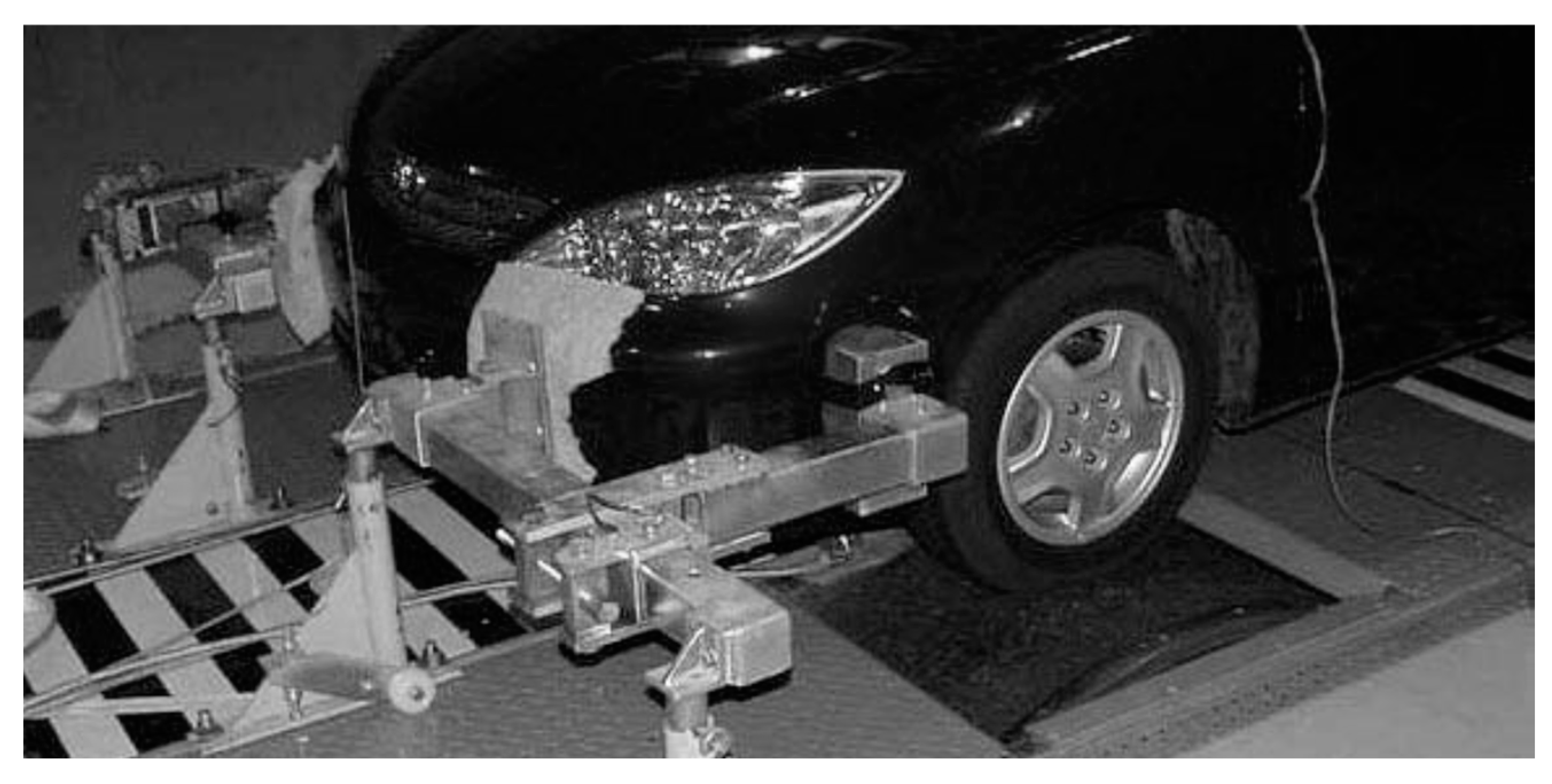Two methods of retaining the test vehicle on a chassis dynamometer are examined in [11]: the typical strap tie-down restraint and an adjustable barrier/corner restraint. The second option is shown in Figure 1. The advantage of employing the barrier/corner design over other types is its minimal effect on the vehicle dynamics. Moreover, it adds no additional loading to the tires. Also, the test vehicle may be accurately centered on the rollers.

The maximum transferable force between the driven wheels and the roller body quantity depends on many factors, such as the vehicle’s restraining points’ heights compared to the location of the vehicle’s center of gravity, as proven in [13]. The free body diagram in Figure 2 demonstrates the forces acting on the test vehicle when using the rear restraint type to avoid introducing an additional vertical load on the tires. Through forces and movement equilibrium, the vertical loads on the front axle (F_z,f) and rear axle (F_z,r) are described in Equation (1).

$$\begin{gathered} F_{z,f}=m g\frac{S_r}{l_w}-F_{rest}\frac{h_{rest}}{l}, \mathrm{w}\mathrm{h}\mathrm{e}\mathrm{r}\mathrm{e} F_{rest}=F_{x,f}+F_{x,r} \\ {F}_{z,r}=m g\frac{S_f}{l_w}+F_{rest}\frac{h_{rest}}{l} \end{gathered}$$

(1)

The traction force on the front axle (F_x,f) is calculated by dividing the driving movement at the front axle by the effective tire radius. The static friction coefficient (μ_h) between the rollers and the tires is assumed to be equal 1, and the height of the vehicle’s center of gravity (h) is experimentally determined to be equal to 0.3 m. The maximum traction force of the front axle (A_V,max) is achieved as in Equation (2). By varying the restraint height (h_rest) and F_rest, we obtain the corresponding A_V,max values, demonstrated by a plane in Figure 3. On the other hand, the demanded driving force (F_x) that equals the driving movement (M_drive) divided by the effective rolling radius (r_e) (i.e., F_x = M_drive/r_e, is a linearly increasing surface independent of h_rest. At the end of the intersection between the A_V,max and F_x surfaces, the range of reachable traction force for a specific μ_h can be identified.

$$A_{V,max}={{\mu }_{h}F}_{z,f}={\mu }_h\left(m g\frac{S_r}{l_w}-F_{rest}\frac{h_{rest}}{l_w}\right)$$

(2)

If the driving movement exceeds the traction potential of the axle, the wheels begin to spin. Furthermore, the vertical loads of the front axle decrease with increases in either h_rest or F_x, while it increases for the rear axle drive, as proven in [13]. In addition, the driving resistance force must be accurately regenerated on the test bench to match real-environment driving. High slipping between the tire and roller will occur when the driving movement exceeds the traction potential. If the slip exceeds a critical slip value, the coating material of the roller and the tire surface will wear faster; so, more errors will occur in the test results [13]. The consequence would be decreased adhesion between the tire and the roller. Therefore, the driving force must always be maintained at less than the maximum transferable force depending on the normal force and the adhesion coefficient. In other words, the frictionally engaged contact between the tire and the roller can critically limit the range of mobility in dynamic driving maneuvers. Therefore, this must be avoided to prevent damaging the coating of the roll surface and the attached tire. Figure 4 shows how much friction influences the traction force capacity. For h_rest = 0.3 m, the maximum F_x is diminished from 5015 N to 3775 N by reducing μ_h from 1 to 0.7.

The modified rolling resistance at the roller is approximated in [2,3] as in Equation (3). The rolling resistance force of the tire on the road (F_R) is affected by the ratio of the unloaded tire radius (r) to the roller radius (R_r) so that an effective rolling resistance on the roller (F_RR) will arise. The accuracy of the calculated rolling resistance on the roller is further improved in [21]. The author added a correction factor e_FR to Equation (3). The simplest form of the proposed correction factor is $e_{FR}=0.195 \frac{p}{F_{Zp}}$, where p is the tire’s pressure (in bars), and F_Zp is the normalized tire’s load (i.e., compared to the full tire’s load) according to the ETRTO (European Tire and Rim Technical Organization (Etrto) https://www.etrto.org/, accessed on 27 November 2023) load standard. More details are available in [21]. Finally, the new effective rolling resistance of the tire on the roller is represented in Equation (4).

$$F_{RR}=F_R{\left(1+\frac{r}{R_r}\right)}^{\frac{1}{2}}$$

(3)

$$F_{RR}=F_R{\left(1+e_{FR}\frac{r}{R_r}\right)}^{\frac{1}{2}}$$

(4)

3. Vehicle Dynamic Model

The electric car shown in Figure 5 is used for research in different automotive engineering and e-mobility-related projects. Besides the technical data of this vehicle, actual maneuver test measurements will be used to validate the developed simulation models. The battery model of the vehicle under the test (VUT) was developed in [22].

According to [23], the calculation of the required driving force for a drivetrain test bench, known as the road load simulation, is based on the equation of motion of the vehicle’s center of gravity in the longitudinal direction. By assuming driving on a dry surface and ignoring the toe-in resistance and the tire rolling resistance part from air ventilation, the total driving force (F_d) is given in Equation (5).

$$F_d=F_A+F_{acc}+F_C+F_R+F_{curve}$$

(5)

The air resistance (F_A) in the longitudinal direction is a function of the front surface area of the vehicle (A_F), air density (ρ), air resistance coefficient with frontal flow wind (C_d), and relative air speed (v_rel). Therefore, Equation (6) puts all terms together.

$$F_A=\frac{1}{2}\rho A_F{c}_d{v}_{A,rel}^2$$

(6)

Acceleration resistance (F_acc) occurs during speed changes so that the vehicle’s inertia acts opposite to the direction of travel. The rotational mass factor (λ*) is significant for considering the additional mass effect from the rotational parts of the vehicle. As a result, the acceleration resistance is obtained as a function of the longitudinal acceleration (a_x), as shown in Equation (7).

$$F_{acc}=m {\lambda }^{*}{a}_x$$

(7)

During acceleration, the engine, i.e., the electric motor in case of an electric powertrain, and other drivetrain parts must also be rotationally accelerated, creating a reaction movement that resists the driving force. This effect is manifested as additional mass to the vehicle’s actual mass (m). According to [24], λ* is expressed in Equation (8). J_E, J_a,f, J_a,r are the inertias of the engine/motor, front axle, and rear axles. i_d, i_g are the gear ratios of the differential gear and the gearbox, respectively. J_C is the total inertia of the coupling elements (i.e., coupling disc, torque convertor, driveshaft, …), and r_e is the effective tire radius. Climbing resistance (F_C) occurs when there is an inclination in the roadway with an angle (α_In). Therefore, Equation (9) represents F_C as a function of the sine of α_In and vehicle weight (F_G).

$${\lambda }^{*}=\left\{\begin{array}{c}\begin{array}{cc}1+\frac{\left(J_{a,f}+J_{a,r}+{i_d}^2{i_g}^2{J}_E\right)}{m {r_e}^2},& \begin{array}{c}no coupling elements between\\ the engine and the differe\end{array}\end{array}\\ \begin{array}{cc}1+\frac{\left(J_{a,f}+J_{a,r}+{i_d}^2{i_g}^2{J}_E\right)}{m {r_e}^2}+\frac{{i_d}^2{J}_C}{m {r_e}^2},& with coupling elements\end{array}\end{array}\right.$$

(8)

$$F_C=F_G\sin {\alpha }_{In}$$

(9)

Considering a nearly linear profile of the rolling resistance across the vertical wheel load F_zW, a load-related characteristic can be defined with the dimensionless rolling resistance coefficient f_RR. According to [25], rolling resistance alternates significantly during dynamic driving maneuvers. For example, it may rise roughly 20% over the steady-state estimated value. Consequently, the rolling resistance tire model proposed in [25] that models the temperature and velocity influences will be employed to accurately estimate the tire’s rolling resistance when mounted on the roller. First, the steady-state rolling resistance (F_R*) is shown in Equation (10). The tire’s steady-state temperature (T*) is then expressed in Equation (11). Next, the tire’s transient state temperature T(t) is found by solving Equation (12). Finally, the rolling resistance force is expressed in Equation (13) as a function of speed, temperature, and vertical load.

$${F_R}^{*}=f_{RR}{F}_{z,W}$$

(10)

$$T^{*}=\frac{{F_R}^{*}{v}_{w0}^k{v}_w^{1-k}}{A_{tire}{h}_0}+T_{amp}$$

(11)

$$v_w{F_R}^{*}\left[1+\epsilon \left(T^{*}-T\left(t\right)\right)\right]-h_0{\left(\frac{v_w}{v_{w0}}\right)}^k{A}_{tire}\left(\left(T\left(t\right)-T_{amp}\right)\right)={m_{tire}c}_{p,tire}\frac{dT}{dt}$$

(12)

$$F_R\left(t\right)={F_R}^{*}\left[1+\epsilon \left(T^{*}-T\left(t\right)\right)\right]$$

(13)

where:

• f_RR—Rolling resistance coefficient;
• F_zW—Normal force on the tire [N];
• A_tire—Outer tire surface area [m²];
• k—Sensibility exponent factor;
• h_0—Reference heat exchange coefficient for rubber and air [W/m²/K];
• ε—Sensitivity of rolling resistance to temperature [1/K];
• c_p,tire—Specific heat transfer factor [J/kg/K];
• F_R(t)—Instantaneous rolling resistance force [N];
• F_R*—Steady-state rolling resistance force [N];
• m_tire—Mass of tire [kg];
• T_amp—Ambient temperature [°C];
• T*—Steady-state operating temperature [°C];
• T(t)—Instantaneous operating temperature [°C];
• v_w0—Reference tire speed [m/s];
• v_w—Tire speed [m/s].

Parameters k and h₀ are determined experimentally in [25] using curve-fitting techniques. The tests were performed at different reference tire speed values. The best results were attained at v_w0 = 80 km/h (22.22 m/s).

The tire is one of the most crucial components in modeling the vehicle’s dynamics. It is the core of vehicle handling and performance since this is the only means of interaction between the car and the ground. Because of its flexibility and pneumatic characteristics, the tire model has highly nonlinear behavior, making it complex to analyze. The so-called Pacejka’s Magic Formula is used to describe the different characteristics of the tires of the VUT.

The contact patch forces of the wheel include the traction force (F_xW), the cornering force (F_yW), the normal force (F_zW), and the self-aligning torque (M_zW). Traction force is a function of slip and normal force. At the same time, the cornering force and self-aligning torque are functions of slip angle and normal force. Magic Formula is an empirical equation often used to represent the contact patch forces, i.e., also known as fore and aft forces, in the tire model. The general form of the magic formula is written in Equation (14).

$$Y=D\sin \left(C\arctan \left(B\varnothing \right)\right), \varnothing =\left(1-E\right) X+\left(\frac{E}{B}\right)\arctan \left(BX\right)$$

(14)

Coefficient D is the maximum peak value of the curve, C determines the shape of the curve, B determines the initial slope of the curve when it is multiplied by factors C and D, and E is the curvature factor that modifies the location of the peak and the curve’s curvature. Y stands for traction force, cornering force, or self-aligning torque. The variable X denotes the slip (κ) for traction force or slip angle (α) in both cornering and self-aligning torque. Coefficients D, C, B, and E are functions of more than 20 other empirical constant values that vary from tire to tire. In addition, the friction effect is incorporated in these coefficients due to the experimental readings. Consequently, it is decided to implement previously estimated values for D, C, B, and E for the model under consideration [25]. When torque is applied to the wheel spin axis, the longitudinal slip κ arises. It can be defined as in Equation (15). The effective rolling radius (r_e) is a value between the free unloaded tire radius (r_f) and the loaded tire radius (r). Longitudinal slip is also defined in Equation (16) as the ratio between the circumferential slip velocity (V_sx) and the forward speed of the wheel center (V_x).

$$\kappa =-\frac{V_x-r_e \Omega }{V_x}$$

(15)

$$\kappa =-\frac{V_{sx}}{V_x}$$

(16)

Figure 6 shows the wheel slip point S attached to the wheel rim. Point S’ is the tire’s contact point, located at the plane’s intersection through the wheel axis and the road plane. The difference in velocities between these two points causes the carcass’ equivalent springs to deflect. Thus, the rate of change in spring deflection for the longitudinal direction of the tire (u) is defined in Equation (17).

$$\frac{du}{dt}=-\left(V_{sx}-V_{sx}^{\prime }\right)$$

(17)

The tire’s stiffness coefficient with the road level generated by the internal elastic force balances the slip forces. For small slip values, longitudinal tire stiffness at the road level can be denoted by (C_Fx), and the longitudinal slip stiffness can be denoted by (C_Fκ). Equation (18) reveals that C_Fκ can be obtained from the longitudinal force (F_xW) versus the slip (κ) curve slope at low slip values, as indicated in [26].

$$C_{F\kappa }={\left(\partial F_{xW}/\partial \kappa \right)}_{\kappa =0}$$

(18)

As in Equation (19), this quantity can be approximated by multiplying the longitudinal Pacejka’s coefficients B_x, C_x, and D_x. The relaxation length is a principal parameter that influences the lag of the response of the slip force to the input slip. Equation (20) expresses the longitudinal relaxation length (σ_κ) under low slip conditions. The differential equation for the deflection u can be derived from Equation (17).

$$C_{F\kappa }=B_x{C}_x{D}_x$$

(19)

$${\sigma }_{\kappa }=\frac{C_{F\kappa }}{C_{Fx}}$$

(20)

The differential Equation (21) defines the relation between u and σ_κ. For linear and small slip conditions, it can be found that the transient longitudinal slip (κ’) and the correspondence F_xW are determined according to Equation (22). The lateral forces will be neglected in this work. At velocity V_x equal or near zero, Equation (21) becomes an integrator. This occurrence could lead to a possibly huge deflection. Certain limitations may be achieved on the longitudinal deflection u in the case of low speeds, i.e., V_x < V_low, and when (21) the deflection exceeds the physically possible values. The slip value at the peak longitudinal force can be roughly estimated using Equation (23) to avoid simulation problems. Factor A has a default value of 1, but a higher value may improve the performance [25]. Based on these results, the identification of σ_κ as expressed in linear Equation (20) can be extended with nonlinear Equation (24). σ_κ0, σ_min are, respectively, the nominal longitudinal relaxation length and the minimum value of the relaxation length introduced to avoid instability and excessive computation. By substituting Equation (22) into (21), the differential Equation (25) is attained.

$$\frac{du}{dt}+\frac{1}{{\sigma }_{\kappa }} \left|V_x\right| u=\left|V_x\right| \kappa =-V_{sx}$$

(21)

$${\kappa }^{\prime }=\frac{u}{{\sigma }_{\kappa }} ,\begin{array}{ccc}& & F_{xW}=\end{array} C_{F\kappa }{\kappa }^{\prime }$$

(22)

$${{\kappa }^{\prime }}_{F_{xW,max}}=A\left(\frac{3D_x}{C_{F\kappa }}\right)$$

(23)

$${\sigma }_{\kappa }=max\left[{\sigma }_{\kappa 0}\left(1-\frac{C_{F\kappa }}{3D_x}\left|{\kappa }^{\mathrm{’}}\right|\right),{\sigma }_{min}\right]$$

(24)

$${\sigma }_{\kappa }\frac{d{\kappa }^{\prime }}{dt}+\left|V_x\right|{\kappa }^{\prime }={-V}_{sx}$$

(25)

At the standstill, the tire acts like a spring, as shown in Figure 7 [27]. This fact can be concluded by verifying using the previously introduced Equation (17) at V_x = 0 that the longitudinal deflection u will act as an integrator $u=-\int V_{sx} dt$ if the lateral deflection is neglected, i.e., V’_sy = 0. The longitudinal force reads $F_{xW}=C_{F\kappa }{\kappa }^{\prime }=\frac{C_{F\kappa }u}{{\sigma }_{\kappa }}$, which is equal to $C_{Fx}u$. These results show that when the tire starts rolling from the standstill, it behaves like a longitudinal or tangential spring and will transform into an artificial damper with a rate of C_Fκ/|V_x|. It shows that the tire damper becomes very stiff at a low speed. At full speed, the tire acts as a damper, while at low speeds, when the tire starts up from a standstill or slows down to a stop, the tire behaves more like a deformable spring, demonstrating a tire transient behavior with a spring-damper system. At very low speeds, the damping decreases when speed is built up. Tire damping is introduced in Equation (26). The damping coefficient k_Vlow should be gradually suppressed to zero when the speed of travel V_x approaches a selected low-value V_low when starting from standstill using Formula (27).

$$\kappa =\left({\kappa }^{\prime }-\frac{k_{Vlow}}{C_{F\kappa }} V_{sx}\right)$$

(26)

$$\begin{array}{ccc}{k}_{V,low}=\frac{1}{2}{k}_{V,low0} \left\{1+cos\left(\pi \frac{\left|V_x\right|}{V_{low}}\right)\right\}& & if \left|V_x\right|\le V_{low}\\ k_{V,low}=0& & if \left|V_x\right|>V_{low}\end{array}$$

(27)

4. Integration of the Complete Vehicle Model

The method employed to estimate the wheel angular speed further improves the concepts developed in [13], considering more detailed models of the driving resistance and the tire. Using only the vehicle’s desired longitudinal velocity (V_x), the corresponding traction force (F_xW), calculated from the tire slip model, will take part in determining the angular speed for each wheel. Figure 8 demonstrates the interaction between the driving movement on the wheel hub (M_drive,i), determined from Equation (5) of the driving resistance model, and the movement from F_xW multiplied by r_e.

As in Equation (28), the rotational speed for the corresponding wheel (ω_i) is estimated by dividing by the wheel hub inertia (J_W), and ω_i is determined according to Equation (29) when the tire slip is taken into consideration. Then, the mechanical power (P_mech) could be estimated according to Equation (30). The sign of the P_mech decides whether the vehicle is driving or braking. In case of driving, the battery must provide an equivalent power that covers the P_mech demands plus power losses (P_loss) of the powertrain. Next, the battery current (I_batt) corresponds to each of the estimated mechanical power; the powertrain power losses and the corresponding battery voltage (V_batt) are estimated using Equation (31). The parameters employed in the test vehicle dynamic model are demonstrated in

Table 1. Parameter list for the VUT dynamic models.

Symbol	Description	Value	Unit
m	Vehicle mass	1528	kg
Jxx	Moment of inertia about the longitudinal axis	482.70	kg·m2
Jzz	Moment of inertia about the vertical axis	2585.60	kg·m2
lw	Wheelbase	2.59	m
Sf	Distance between center of gravity and front axle	1.47	m
Sr	Distance between center of gravity and rear axle	1.11	m
h	Height of the vehicle’s center of gravity	0.45	m
ig	Transmission gear ratio	4	-
id	Differential gear ratio	2.5	-
Je	Vehicle engine/motor inertia	0.03	kg·m2
Ja,f	Front axle inertia	3.7 × 10−3	kg·m2
Ja,r	Rear axle inertia	3.7 × 10−3	kg·m2
JT	Tire inertia	0.1	kg·m2
JW	Wheel hub inertia	0.124	kg·m2
hW	Height of the vehicle’s rolling center	0.31	m
SW	Half-track width between front wheels or rear wheels	0.78	m
SF,f	Distances of the front suspension from the middle	0.78	m
SD,f	Distances of the front damper from the middle	0.78	m
SF,r	Distances of the rear suspension from the middle	0.78	m
SD,r	Distances of the rear damper	0.78	m
cF,f	Spring stiffness front	21,269	N/m
dD,f	Damping coefficient front	2244.4	N·s/m
cSt,f	Stiffness of the front anti-roll bar	7018.8	N·m/rad
cF,r	Spring stiffness rear	17,374	N/m
dD,r	Damping coefficient rear	1550.6	N·s/m
Bx	Longitudinal force initial slope in Pacejka formula	23.64	-
Cx	Longitudinal force shape factor in Pacejka formula	1.35	-
Dx	Longitudinal force peak factor in Pacejka magic formula	0.90	-
Ex	Longitudinal force curvature factor in Pacejka formula	1.37	-
Bz	Aligning initial torque slope in Pacejka formula	16.37	-
Cz	Aligning torque shape factor in Pacejka formula	1.13	-
Dz	Aligning torque peak factor in Pacejka magic formula	0.13	-
Ey	Aligning torque curvature factor in Pacejka formula	0.89	-
re	Tire effective rolling radius	0.31	m
CFx	Tire longitudinal stiffness factor (related to the wheel load)	19.15	1/m
σκ0	Tire longitudinal nominal relaxation length	1.5	m
σmin	Tire minimum relaxation length	0.05	m
Vlow	Low-speed threshold	2.50	m/s
kV,low0	Damping coefficient at low speed	770	N·s/m

.

$$J_W {\dot{\omega }}_i=M_{drive,i}-F_{xW,i} r_e$$

(28)

$${\omega }_i=\int \frac{1}{J_W}\left(M_{drive,i}-F_{xW,i} r_e\right)dt$$

(29)

$$P_{mech}={\sum }_1^4{M}_{drive,i} {\omega }_i$$

(30)

$$I_{batt}=\frac{P_{mech}+P_{loss}}{V_{batt}}$$

(31)

The total cumulative energy consumption E(t) is calculated as integrating the total power over time, as shown in Equation (32). Equation (33) describes the instantaneous power at the time (t). Since this work focuses on estimating the consumed energy, the regenerative functionality is disabled in the VUT. Therefore, the simulation models will not employ the relevant equations for regenerative braking and the generator mode of the car’s electric machine.

$$E\left(t\right)={\int }_{t_0}^t{P}_{ins}\left(\tau \right)d\tau$$

(32)

$$P_{ins}\left(t\right)=\left\{\begin{array}{cc}\frac{P_{mech}\left(t\right)}{{\eta }_{pe}{\eta }_g{\eta }_{mot}\left(x\right)f_{norm}}+P_{aux} ,& P_{mech}\left(t\right)\ge 0 \left(driving\right)\\ \begin{array}{ccccccc}& & 0& & & & ,\end{array}& P_{mech}\left(t\right)<0 \left(braking\right)\end{array}\right.$$

(33)

where:

• P_ins—Total powertrain’s power (electrical power at the battery);
• P_mech—Mechanical power (mechanical power at the output of the motor–gearbox unit);
• η_pe—Power electronics’ efficiency;
• η_g—Gearbox efficiency;
• η_mot—Motor efficiency;
• x—Fraction of the motor’s mechanical power;
• f_norm—Normalization factor;
• P_aux—Auxiliary power.

The wheel load (F_zW) is significant in calculating the contact patch forces. The location of the vehicle’s CG plays a primary role in distributing the total vehicle weight F_G among the wheels. The geometrical distance from the CG to the front axle (S_f), the distance to the rear axle (S_r), and the height of the center of gravity (h) are shown in Figure 9. The influence of the air drag lifting effect is not taken into consideration. The wheel loads on the front axle are obtained by creating the torque balance around the contact point of the rear axle tires. Analogously, the wheel loads of the rear axle are obtained by forming the movement equilibrium around the contact point of front axle [28,29].

Road inclination and vehicle acceleration cause a change in the axle load distribution, which makes the axles’ loads have static and dynamic parts. The static part for each front and rear axle is calculated using Equations (34) and (35). Wheel load is also affected by acceleration; so, acceleration force acts on the vehicle’s center of mass opposite the direction of acceleration. Consequently, the dynamic part of the axles’ vertical load [24,28] is as shown in Equations (36) and (37). λ* is determined using Equation (8). Then, by summing the static terms in Equation (34) together with the dynamic terms (36) and by carrying out the same process for Equations (35) and (37), we obtain the total axle loads equations as expressed in Equations (38) and (39).

$$F_{z,f/static}=\frac{S_r}{l_w}{F}_G cos{\alpha }_{In}-\frac{F_G}{l_w}hsin{\alpha }_{In}$$

(34)

$$F_{z,r/static}=\frac{S_f}{l_w}{F}_G cos{\alpha }_{In}+\frac{F_G}{l_w}hsin{\alpha }_{In}$$

(35)

$$F_{z,f/dynamic}=-m a_x \frac{h}{l_w}$$

(36)

$$F_{z,r/dynamic}=m a_x \frac{h}{l_w}$$

(37)

$$F_{z,f/total}=\frac{S_r}{l_w}{F}_G cos{\alpha }_{In}-\frac{F_G}{l_w}hsin{\alpha }_{In}-m a_x \frac{h}{l_w}$$

(38)

$$F_{z,r/total}=\frac{S_f}{l_w}{F}_G cos{\alpha }_{In}+\frac{F_G}{l_w}hsin{\alpha }_{In}+m a_x \frac{h}{l_w}$$

(39)

5. Generic Energy Consumption Model for the Electric Powertrain

The authors of [30] proposed a computational model for energy consumption in EVs. They introduced a generic battery model based on technical data. The model’s accuracy is promoted by incorporating the technical specifications of electric machines, which are employed to generate efficiency curves for both motor and generator operation phases. In this work, the model proposed in [30] will be improved by incorporating more detailed driving resistance and battery models.

Electric motors are generally designed to operate between 50 and 100% of their rated load, with the highest operating efficiency at roughly 75% of the full load. At the same time, the motor efficiency decreases severely at loads below 50%. The part-load efficiency curves are presented in Figure 10 for typical electric motors with different rated power values [30]. The motor efficiency can be estimated, according to [30], as a function of the fraction (x) of the mechanical output power of the motor (P_mo) in W concerning the rated motor power (P_mr) in kW, i.e., x = 0.001|P_mo|/P_mr. Equation (40) describes the generalized electrical machine efficiency for either motor mode (η_mot) or generator mode (η_gen).

$$efficiency\left(x\right)=\left\{\begin{array}{cc}\frac{cout1 x+cout2}{x+cout3} ,& 0\le x<0.25\\ dout1 x+dout2 ,& 0.25\le x<0.75\\ eout1 x+eout2 ,& x\ge 0.75\end{array}\right.$$

(40)

The coefficients in Equation (40) are acquired in [30] from the curve fitting of several motors and are presented in

Table 2. Coefficients for determining efficiency in Equation (40) [30].

	Induction Electric Machine		Synchronous Electric Machine
Coefficient	Motor Mode	Generator Mode	Motor Mode	Generator Mode
cout1	0.924300	0.925473	0.942269	0.942545
cout2	0.000127	0.000148	0.000061	0.000067
cout3	0.012730	0.014849	0.006118	0.006732
dout1	0.080000	0.075312	0.060000	0.057945
dout2	0.860000	0.858605	0.905000	0.904254
eout1	−0.073600	−0.062602	−0.076000	−0.066751
eout2	0.975200	0.971034	1.007000	1.002698

. One of the electrical machines’ main characteristics is that their efficiency increases with size [31]. Therefore, when calculating the efficiency for an electrical machine with specific output power, the efficiency must first be attained from Equation (40), then multiplied by a normalization factor (f_norm). While in the case of regenerative braking, the efficiency must be multiplied by a regenerative normalization factor (f_regen), as explained in [30]. Figure 11 displays the efficiency normalization factor based on rated output power.

The mechanical energy losses from the total gears transmission efficiency (η_g) are also significant [32]. Therefore, the authors of [33] also developed an energy consumption model for EVs with a deceleration-dependent regenerative braking efficiency model. They validated their model with different electric vehicles over several typical driving cycles. In addition, they analyzed the impact of auxiliary systems load on energy consumption by performing the simulation at three different ambient temperatures. Accordingly, the total battery output should also supply the auxiliary load power (P_aux) and supply the power for the motor or to receive the electrical power from the generator. In [34], the power model is multiplied by a correction factor constant to consider the drop in battery efficiency during the round trip, while in this work, a detailed battery model, introduced in the following section, is employed as the proposed battery model incorporates more variable loss factors. The front-wheel-driven VUT has an asynchronous machine; its specifications are listed in

Table 3. Technical data of the used VUT electric motor.

Parameter	Value
Rated Power	45 kW
Peak Power	68 kW
Peak Torque	210 N·m
Rated Speed	3000 RPM
Number of poles	6

. The losses within the power electronics components occur due to converting the direct current from the battery into a three-phase current to the motor. Therefore, the efficiency characteristics of the power electronics (η_pe) can be mapped via an efficiency map analogous to the map of the electric machine, as shown in Figure 12. The data in this figure are determined for a motor with a maximum power of 100 kW. However, the efficiency of power electronics for a powertrain with lower motor power can also be estimated from Figure 12 [35]. Each dashed line expresses the same efficiency of all points spreading on it. The red zone demonstrates the high-efficiency working points, followed by the yellow area, and finally comes the lowest efficiency, represented by the light-blue zone.

Figure 11. Normalization factor (f_norm) curve [34].

Figure 11. Normalization factor (f_norm) curve [34].

6. Evaluation of the Testing Results from the Roller Dynamometer Test Bench

The evaluation is made with the Mercedes A-Class test vehicle’s experimental NEDC and WLTP2 driving cycles. The restraint used in this experiment is shown in Figure 13, which does not apply any additional vertical loads to the tires. Moreover, the vehicle’s center of gravity height (h_CG) is estimated at 0.45 m, while the restraint point (h) height equals 0.3 m.

6.1. NEDC and WLTP2 Driving Cycles Results from the Dynamometer Test Bench

The first performed driving cycle is the NEDC. It can be seen from Figure 14 that the reference speed profile is tracked with a good performance with a mean square error of 0.6858 km/h. The validated model for the VUT would be advantageous in assessing the plausibility of the test measurement results.

It can be seen from Figure 15 that the total reaction forces on the rollers attached to the front tires (corresponding to F_x,f and F_x,r in Figure 2) reach relatively lower positive values than the expected values from the VUT model during acceleration. While braking, the force behavior matches the expectations from the simulated street driving of the VUT. The divergence between the measured and the simulated forces is ascribed to the fact that the influence of the rolling resistance force of the tires is not captured in the measurements. Correspondingly, the mechanical power measured from the test bench system (P_Trac,Dyno), which is determined by multiplying the measured traction force by the measured vehicle’s speed, has relevant mismatches with the street driving estimated mechanical power (P_Mech,Street) of the same driving cycle estimated via Equation (5), as shown in Figure 16. The test bench automation system is calibrated by executing a group of coast-down tests on the VUT prior to the desired maneuver tests. Nevertheless, this did not change the fact that the VUT underwent different driving resistances compared to those of street driving, which dictates the need to implement specific corrections on the dynamometer test bench results for the purpose of simulating the corresponding street driving maneuvers. It is worth mentioning that high slipping between the tires and rollers was observed during the experimental test period, from 894 to 1160 s, which is expected to cause an error in power estimation for the high-speed part of the cycle.

Next, the WLTP2 test was performed on the same car. This test was explicitly chosen because it has a lower maximum speed (85 km/h) than the NEDC cycle (120 km/h). Moreover, WLTP2 is more dynamic than the NEDC cycle. Consequently, the slipping due to high speed would be reduced in this maneuver, and the acceleration influence on the slip (due to the more dynamic course) could be emphasized. Figure 17 shows the speed tracking accuracy for the WLTP2 reference driving cycle, which also performed well.

Figure 18 illustrates the measured reaction force from the test bench and the expected traction force for the validated VUT model for the street driving simulation. Since the test bench reacted the same way as it did with the NEDC cycle, the diagram for comparing the power for the WLTP2 cycle is omitted here. It was shown in [36] that significant divergences exist between the on-road emissions and fuel consumption measurements and the driving cycles’ measurements on the chassis dynamometer. It was also proven in [20] that slip at the contact point between the vehicle’s tires and the dynamometer’s rollers leads to unmanageable inconsistency in emission measurements, while tightening the vehicle restraints may increase emissions and energy consumption.

A conclusion was made in [37] that the uncertainty in determining the road load coefficients, i.e., typically the so-called ABC factors, will significantly affect the reliability of the test measurements for the vehicle system. In addition, a comparison was made in [38] between the on-road data and the measured fuel consumption and pollutant emission from the roller dynamometer for 16 different vehicles. The comparison criteria are based on the vehicle’s specific power and portable emission measurement systems. The vehicles under the test underwent the NEDC and WLTP-class two (WLTP2) driving cycles on a chassis roller dynamometer. The results show significant differences between street measurements and driving cycle measurements, especially for internal combustion engine vehicles. As a final point, it must be indicated that chassis dynamometers are continuously moving away from being employed as certification tools, development platforms for calibration, or system optimization and validation tasks [1,2,39].

6.2. Improving the Roller Dynamometer Test Bench Results

It was previously presented that there are several limitations and sources of errors when testing with the chassis dynamometer. Slip estimation is the major problem that caused the substantial mismatch between the expected and the measured energy consumption. Therefore, an analytical study and additional adjustments are proposed in the tire model in this section to interpret the deviation of the actual testing measurements on chassis dynamometers from the expected results from street driving. So, to compensate for this difference, the additional power calculated from the rolling resistance model in Equation (13) (i.e., $F_R{V}_x$, valid for the flat road surface) with the correction Equation (4) is added to the results of the roller test bench (i.e., $P_{Mech,Dyno}=(DYNO Measured force+F_{RR})·V_x$, valid for the curved road surface of the roller dynamometer). Consequently, the estimated mechanical power from the roller dynamometer leads to results that match the simulation of the VUT model very well, as demonstrated in Figure 19. Therefore, the proposed power estimation models of the street driving and the roller dynamometer should have analogous results when estimating the total power consumption P_ins determined from Equation (33), as Figure 20 and Figure 21 show.

The root means squared error concerning Pins between the test bench with respect to the street driving estimation concerning the VUT model (RMSE_Dyno,Street) is determined for both NEDC and WLTP2 tests. The results in

Table 4. RMSE_Dyno,Street for both NEDC and WLTP2.

NEDC	WLTP2
0.6553 [kW]	0.7504 [kW]

show that the error between the estimated P_Total,Dyno and the expected P_Street is higher in the WLTP2 driving cycle due to its dynamic attribute.

7. A Proposed Approach for Estimating the Friction between the Tire and the Roller

It has been presented in the last sections that testing using the chassis dynamometer has several limitations and sources of errors. Therefore, an analytical study and additional adjustments are proposed in this section to interpret the deviation of the actual testing measurements on chassis dynamometers from the expected results from street driving.

7.1. Friction Tire Model

Friction is a complex interaction between the surface and the near-surface regions of two bodies moving relative to each other. The tire dynamic friction model [40,41,42] combines the Dahl model [41] with steady-state friction characteristics, which comprises both the tire’s transient and steady-state behavior. In addition, the authors developed an ordinary differential equation called the LuGre model [42], a surface- and velocity-dependent model on the contact patch length (L) between the tire and the ground to approximate the distributed friction model, as represented in Figure 22. This model simulates several longitudinal tire friction phenomena, such as the Stribeck effect, spring-like characteristics, and stick-slip motion. As shown in Figure 23, the ‘Stribeck effect’ [43] appears as a drop in the forces at low speeds. A Stribeck relative velocity parameter (i.e., the velocity of the tire surface relative to the velocity of the tire’s body, as defined in Equation (41)) shapes the Stribeck curve. Moreover, it incorporates the tire’s longitudinal lumped stiffness (σ₀) and a viscous damping factor relative to the longitudinal speed (σ₂). This tire model also includes a viscous damping term g(s) as a function of longitudinal slip (s), static friction coefficient (μ_h), Coulomb friction coefficient (μ_c), and the Stribeck relati ve velocity (v_s).

The model proposed in [42] distinguishes between driving and braking modes based on the relative speed (v_r). In [42], the slip (s) is defined according to Equation (42). The wheel rotational speed (ω) is evaluated as elaborated previously. After that, the driving modes, i.e., driving, braking, or standstill modes, are classified according to the test car’s acceleration and deceleration measurements. Since the slip (κ) estimation is more extensively defined in Pacejka’s model than in Equation (42), it will be employed instead.

$$v_r=r_e\omega -V_x$$

(41)

$$s=\left\{\begin{array}{cc}{s}_d=1-\frac{V_x}{r_e\omega },& for driving\\ & \\ s_b=\frac{r_e\omega }{V_x}-1,& for braking\end{array}\right.$$

(42)

The uniform load LuGre friction model is described in Equations (43) and (44) for driving mode and Equations (45) and (46) model the tire friction in the braking mode [40]. The tire’s contact patch is different for roller contact (L_LT) than for flat surface contact (L_LE), as shown in Figure 24. The ratio between the two cases is also estimated in [20] with a correction factor e_Cα, as shown in Equation (47). This concept is employed in this work to estimate the variable (L) in Equations (43) and (45), which enables a comparison between on-road testing and the rollers of the dynamometer.

$$F_d\left(s\right)=\left(sgn\left(v_r\right)g\left(s\right)\left(1+\frac{g\left(s\right)}{{\sigma }_{0}L\left|s_d\right|}\left(e^{-\frac{{\sigma }_{0}L\left|s_d\right|}{g\left(s\right)}}-1\right)\right)+{\sigma }_2{r}_e\omega s_d\right)F_z$$

(43)

$$g\left(s\right)={\mu }_c+\left({\mu }_h-{\mu }_c\right)e^{-{⌊\frac{r_e\omega s_d}{v_s}⌋}^{0.5}}$$

(44)

$$F_b\left(s\right)=\left(sgn\left(v_r\right)g\left(s\right)\left(1+\frac{g\left(s\right)\left|1+s_b\right|}{{\sigma }_{0}L\left|s_b\right|}\left(e^{-\frac{{\sigma }_{0}L\left|s_b\right|}{g\left(s\right)\left|1+s_b\right|}}-1\right)\right)+{\sigma }_2{V}_x{s}_b\right)F_z$$

(45)

$$g\left(s\right)={\mu }_c+\left({\mu }_h-{\mu }_c\right)e^{-{⌊\frac{V_x{s}_b}{v_s}⌋}^{0.5}}$$

(46)

In this work, the LuGre model parameters μ_h, μ_c, v_r and L_LE are set to 1.29, 0.93, 3.72 m/s and 0.2 m, respectively, according to [41]. Based on [21], with a tire pressure of 2.2 bar and 100% load according to the ETRTO standards, the correction factors e_FR and e_Cα are determined as 0.52 and 0.10, respectively. Then, Equation (47) is employed to determine the L_LT value corresponding to the given L_LE value. It was proven that the LuGre model is very efficient in modeling braking behavior, especially in extreme maneuvers. Therefore, two tire models are employed as in [17]: one for driving and the other for braking. First, the LuGre model is used for driving and braking but with different parameters. Then, the parameters σ₂, and σ₀ are manually tuned to 0.2 s/m, and 210 m⁻¹, respectively, until the best fitting between the experimental and simulated power consumption is achieved for the driving part of the maneuver. Next, by tuning the braking part of the LuGre model, it is found that only by reducing σ₀ to 130 m⁻¹ and using the same parameters as for the driving part is an accurate estimation of the braking dynamic achieved. Figure 25 demonstrates the proposed model for the total power estimation process of the VUT under the chassis dynamometer testing conditions.

$$\frac{L_{LE}^2}{L_{LT}^2}=1+e_{C\alpha }\frac{r}{R_r}$$

(47)

7.2. Influence of the Roller on the Temperature of the Tire

The tires can heat up severely during dynamic test runs, which must be monitored during the test run [13]. Furthermore, solving the paradox of avoiding an additional vertical load by the employed restraint type and excessive slip between the tire and the roller is still a challenging issue. So, the rolling resistance model, i.e., Equations (10)–(13), is employed to compare the estimated rolling resistance for street driving and the tire rotating on the roller simulation. For the dynamometer testing simulation, L_LT is used instead of L_LE in Equations (43) and (45), and then the correction in Equation (3) is applied. There is also a noticeable increase in the rolling resistance in the dynamometer simulation compared to the street driving simulation by 15%, which leads to more heating for the tires in roller dynamometer testing, as shown in Figure 26 and Figure 27.

The proposed simulation model estimates the test tire’s friction forces and the slip between the tire and roller, enabling a more accurate estimation of the actual energy consumption on the roller dynamometer test bench. Furthermore, it estimates some essential physical properties during the testing process, such as the tire’s temperature, which can help to monitor these quantities if the relevant measurement technologies are unavailable.

8. Validation of the Simulation Models

The next step is to compare the total estimated power, i.e., mechanical power and powertrain losses, with the measured power from the VUT battery during both NEDC and WLTP2 driving cycle tests. In other words, the reliability of the proposed simulation models for different driving maneuvers is validated in this section.

8.1. Validation of the Enhanced Power Estimation Model for the Roller Dynamometer Measurements

It is then desired to assess to which scale the direct measurements of the electrical power consumption from the VUT battery on the roller test bench may be estimated based on the direct force and speed measurements in combination with other simulated driving resistances and power losses. These results are shown for both NEDC and WLTP2 driving cycle tests in Figure 28 and Figure 29, respectively. Obviously, the most considerable divergence occurred in the higher-speed parts of the tests, as shown in Figure 28a. At the same time, the errors are distributed along the WLTP2 test in Figure 29a. On the other hand, the actual braking impact on the VUT was less than expected. These differences between the actual and the estimated results are ascribed to the excessive slipping of the tires on the rollers. As a result, Figure 28b and Figure 29b indicate that the battery power consumption during acceleration is higher than the estimated total power, which is attained from the measured mechanical power, followed adding the power losses according to Equation (33), as demonstrated in Section 6.2. Moreover, some measured power pinpoints in the positive range are not captured in the force measurements, which made them unpredictable for the model. This deviation is attributed to insufficient measured entries for the model. Only two actual measured quantities are provided on the test bench: the traction force on each tire F_xW; and the rollers’ rotational speed, which is used to estimate the vehicle’s speed. So, there is no physical measurement system for the tires. These form sources of inaccuracy in the estimation results no matter how detailed and precise the model is. For instance, it is well established that tire rolling resistance can only be adequately measured with a specialized apparatus [45]. It is then expected to have some errors from the rolling resistance model shown in Equation (13) due to inaccurate entries, such as the actual vehicle speed v_w.

Despite these, Figure 28c displays a very good match between the measured P_Battery and estimated P_Total,Dyno, with a Pearson correlation coefficient (Pearson correlation coefficient—Wikipedia, https://en.wikipedia.org/wiki/Pearson_correlation_coefficient#cite_note-3, accessed on 27 November 2023) (ρ_X,Y) of 0.951 for the NEDC cycle, and a correlation of 0.976 for the WLTP2 driving cycle, as shown in Figure 29c. The error in Figure 28a is more significant at the last part of the NEDC, where the speed is higher than the rest of the test, and the expected negative braking power is mostly more extensive than the measured. This caused an unsymmetric error distribution that is shifted more to the positive error portion, as shown in Figure 28d. These observations indicate that the testing on the roller dynamometers causes higher energy consumption than expected. Although the WLTP2 has a lower maximum speed than the NEDC driving cycle, it caused a more significant difference, i.e., about four times, between the measured and expected values, as illustrated in Figure 29d compared to Figure 28d. This outcome is attributed to the fact that the WLTP2 is more dynamic than the NEDC driving cycle. This, in turn, increases the possibility of more unforeseen slipping incidents between the tires and the rollers than expected from the simulation models.

8.2. Validation of the Proposed Power Consumption Model

Figure 30 shows that by employing the LuGre model with the proposed adjustments, the instantaneous power is accurately predicted for the NEDC cycle test. The matching between the proposed model and the measured data is evident in Figure 30a–d. Moreover, the errors from the high-slipping period, from 894 to 1160 s (see Figure 16), are significantly reduced compared to the results from the street model, as shown from the perfect correlation in Figure 30c that reached about 0.99 and the minimal difference between the measurements and the estimated signals, shown in Figure 30d. In addition, the negative power part, representing the braking mode, is more fitting to the measured values. Subsequently, the overall results in Figure 30 demonstrate a substantial improvement compared to the performance of the VUT in Figure 28. Likewise, Figure 31 illustrates an excellent association between the actual measurements from the WLTP2 test and the simulated results from the proposed model. The correlation in Figure 30c is about 0.984, and the difference in Figure 30d has significantly improved in contrast to the results in Figure 29d. Nonetheless, slight divergences are still present due to the uncertainty of the slip quantity between the tires and the rollers.

Table 5. RMSE_Street,VUT and RMSE_LuGre,VUT for both NEDC and WLTP2.

	NEDC	WLTP2
RMSEDyno,VUT	1.2929 [kW]	1.3499 [kW]
RMSELuGre,VUT	0.4366 [kW]	0.5599 [kW]

summarizes the root mean squared error of the total estimated power from the street driving model (RMSE_Street,VUT), and the RMSE of the total estimated power from the proposed model (RMSE_LuGre,VUT), both with respect to the measured power from the battery of the VUT. These values confirm the significant improvement in power estimation accuracy, which complies with the observations in Figure 28, Figure 29, Figure 30 and Figure 31.

9. Conclusions

The capacities of the chassis dynamometer test benches as a testing environment are investigated in this work. An intensive literature review for the state of the art is carried out with an emphasis on the limitations of testing using chassis dynamometers. This work contributes to two central points: First, analytical and experiment evaluations are performed systematically in this research by creating detailed simulation models and evaluating the results based on experimental measurements. The analysis shows that chassis dynamometers suit dynamic driving maneuvers under certain conditions. In particular, the more the test incorporates dynamic driving maneuvers, the higher the errors in the roller test bench results. The results revealed that testing on the roller dynamometers produces higher energy consumption than testing on a flat surface, confirming the literature review’s observations. Even though the NEDC has a higher maximum speed than the WLTP2 driving cycle, a more significant difference between the measured and expected results occurs in the WLTP2 case since it is more dynamic. In order to better simulate the tire’s dynamic behavior on the roller, the implemented LuGre friction model has two different sets of equations with different parametrization: one for the driving mode, and the other one for the braking mode. The modifications to the uniform load LuGre friction model, which is the second central point of this work, are summarized in three key contributions: First, it was modified to be adapted to the roller dynamometer test bench by adjusting the contact patch length to the concaved roller radius according to the ETRTO -standards and optimized correction factors for roller test benches. Second, the vertical load on the axles, influenced by the restraint system, is considered. Third, the nonlinear slip estimation from the Pacejka tire model is implemented instead of the simplified slip definition in the LuGure model, considering splitting the Pacejka slip signal between driving and braking slip signals. The proposed LuGre tire model is integrated with a larger-scale physical generic power consumption model. The proposed model comprises a dynamic physical model for the mounted vehicle on the chassis dynamometer, a driving resistance model, a power loss model of the electric powertrain, a LuGre distributed friction tire model which considers the load distribution on the contact patch length between the tire and the ground, and a correction for the contact patch length between the wheel and the roller. Given only the measured speed of the test cycle and the corresponding auxiliary power consumption, the proposed model demonstrates high accuracy in estimating the actual measured power. Nevertheless, some different potential sources of errors still exist due to the curvature geometry of the roller, which has several influences, such as increasing the tire’s rolling resistance force compared to driving on a flat surface. Furthermore, inaccurately estimating the vehicle’s speed leads to errors in tire slip estimation, influencing the final power estimation results. Another source of dissimilarities in results is the slipping between the tire and the roller, which is a major source of uncertainty that diminishes the accuracy of estimating the energy consumption in the roller dynamometer test benches. The influences of these divergences can only be predicted with a more advanced measurement apparatus that provides the necessary information.

This research established a comprehensive basis for future work: implementing this approach for other types of vehicles, such as buses and trucks. Moreover, the proposed model can be extended by considering the regenerative braking system and investigating its influence on the braking time. Furthermore, this method could be employed to estimate energy consumption for other powertrain types: internal combustion engines, fuel cells, and hybrid powertrains. In addition, a methodology to mitigate the investigated limitations of the roller test bench, such as advanced calibration techniques or integrating additional sensors, could be proposed. Also, this method could be used in real-world driving scenarios by incorporating a three-dimensional route profile and different driving resistances on the tires, and, finally, modeling the auxiliary power instead of relying on the measurements for every new test maneuver or test conditions.

References

1. Mayyas, A.; Prucka, R.; Pisu, P.; Haque, I. Chassis Dynamometer as a Development Platform for Vehicle Hardware In-the-Loop VHiL. SAE Int. J. Commer. Veh. 2013, 6, 257–267. [Google Scholar] [CrossRef]
2. Paulweber, M.; Lebert, K. Powertrain Instrumentation and Test Systems, 1st ed.; Springer International Publishing: Berlin/Heidelberg, Germany, 2016; ISBN 978-3-319-32133-2. [Google Scholar]
3. Düser, T.; von Gravel, R.; Haase, A.; Olms, H.; Schmidt, C.; Schmidt, U. Fahrzeugrollenprüfstände: Von der Zertifizierung bis hin zur Mechatronischen Entwicklungsplattform; Verlag Moderne Industrie (mi connect): Landsberg, Germany, 2011; ISBN 978-3-86236-022-2. [Google Scholar]
4. Bauer, S.; Beidl, C.; Düser, T. Methodik zur Erzeugung RDE-Relevanter Szenarien im Prüfstandsumfeld. In Simulation und Test 2017; Springer Vieweg: Wiesbaden, Germany, 2018. [Google Scholar] [CrossRef]
5. Maschmeyer, H.; Beidl, C.; Düser, T.; Schick, B. RDE-Homologation—Herausforderungen, Lösungen und Chancen. MTZ—Mot. Z. 2016, 77, 84–91. [Google Scholar] [CrossRef]
6. Weber, T.; Beidl, C.; Düser, T.; Gietzelt, C. The Chassis Dynamometer as Real World Driving Environment. In 14. Internationales Stuttgarter Symposium; Springer Vieweg: Wiesbaden, Germany, 2014; pp. 1641–1662. [Google Scholar]
7. Lensch-Franzen, C.; Schintzel, K.; Rosner, A. Applikationsoptimierung für aktuelle Anforderungen im Antriebsstrang. MTZ—Mot. Z. 2018, 79, 42–47. [Google Scholar] [CrossRef]
8. Brace, C.J.; Burke, R.; Moffa, J. Increasing accuracy and repeatability of fuel consumption measurement in chassis dynamometer testing. Proc. Inst. Mech. Eng. 2009, 223, 1163–1177. [Google Scholar] [CrossRef]
9. Martyr, J.; Plint, M.A. Engine Testing: The Design, Building, Modification and Use of Powertrain Test Facilities. In Engine Testing; Elsevier: Amsterdam, The Netherlands, 2012. [Google Scholar] [CrossRef]
10. Nakajo, T.; Tsuchiya, K. Factors Affecting Driving Force Characteristics of 4WD Vehicles on a 4WD Chassis Dynamometer; SAE International: Warrendale, PA, USA, 2009. [Google Scholar]
11. Hendrick, D.; Vennefron, A.; Sienkiewicz, D. Vehicle Retention Methods for Four-Wheel Chassis Dynamometer Testing; SAE International: Warrendale, PA, USA, 2003. [Google Scholar]
12. Pexa, M.; Mader, D.; Čedík, J.; Peterka, B.; Müller, M.; Valášek, P.; Hloch, S. Experimental verification of small diameter rollers utilization in construction of roller test stand in evaluation of energy loss due to rolling resistance. Measurement 2020, 152, 107287. [Google Scholar] [CrossRef]
13. Pillas, J. Modellbasierte Optimierung Dynamischer Fahrmanöver Mittels Prüfständen; Shaker: Cleveland, OH, USA, 2017; ISBN 978-3-8440-5420-0. [Google Scholar]
14. Sato, Y.; Kusakabe, T.; Satonaka, T.; Nakamura, S.; Ogawa, Y.; Noguchi, S. An Analysis of Behavior for 4WD Vehicle on 4WD-Chassis Dynamometer; SAE International: Warrendale, PA, USA, 2010. [Google Scholar]
15. Gao, X.; Xiong, Y.; Liu, W.; Zhuang, Y. Modeling and experimental study of tire deformation characteristics under high-speed rolling condition. Polym. Test. 2021, 99, 107052. [Google Scholar] [CrossRef]
16. O’Neill, A.; Prins, J.; Watts, J.F.; Gruber, P. Enhancing brush tyre model accuracy through friction measurements. Veh. Syst. Dyn. 2022, 60, 2075–2097. [Google Scholar] [CrossRef]
17. Yamashita, H.; Matsutani, Y.; Sugiyama, H. Longitudinal Tire Dynamics Model for Transient Braking Analysis: ANCF-LuGre Tire Model. J. Comput. Nonlinear Dyn. 2015, 10, 031003. [Google Scholar] [CrossRef]
18. de Menezes Lourenço, M.A.; Eckert, J.J.; Silva, F.L.; Santiciolli, F.M.; Silva, L.C.A. Vehicle and twin-roller chassis dynamometer model considering slip tire interactions. Mech. Based Des. Struct. Mach. 2023, 51, 6166–6183. [Google Scholar] [CrossRef]
19. Eckert, J.J.; Bertoti, E.; Costa, E.d.S.; Santiciolli, F.M.; Yamashita, R.Y.; de Alkmin e Silva, L.C.; Dedini, F.G. Experimental Evaluation of Rotational Inertia and Tire Rolling Resistance for a Twin Roller Chassis Dynamometer. In SAE Technical Paper Series, Proceedings of the 26th SAE BRASIL Inernational Congress and Display, São Paulo, Brasil, 7 November 2017; SAE International400 Commonwealth Drive: Warrendale, PA, USA, 2017. [Google Scholar]
20. Nehlsen, M.; Jedicke, F.; Bogner, E.; Schöggl, P. Fahrbarkeitsuntersuchungen auf dem Rollenprüfstand. ATZ Automob. Z. 2006, 108, 376–381. [Google Scholar] [CrossRef]
21. Unrau, H.-J. Der Einfluss der Fahrbahnoberflächenkrümmung auf den Rollwiderstand, die Cornering Stiffness und die Aligning Stiffness von Pkw-Reifen; KIT Scientific Publishing: Karlsruhe, Germany, 2013; ISBN 978-3-86644-983-1. [Google Scholar]
22. Alhanouti, M.; Gießler, M.; Blank, T.; Gauterin, F. New Electro-Thermal Battery Pack Model of an Electric Vehicle. Energies 2016, 9, 563. [Google Scholar] [CrossRef]
23. Bauer, R. New Methodology for Dynamic Drive Train Testing; SAE International: Warrendale, PA, USA, 2011; pp. 1–6. [Google Scholar]
24. Meywerk, M. Vehicle Dynamics, 1st ed.; John Wiley & Sons: Hoboken, NJ, USA, 2015; ISBN 978-1118971352. [Google Scholar]
25. Andrea, M.F.; Lienkamp, M. Rolling resistance modeling for electric vehicle consumption. In 6th International Munich Chassis Symposium 2015; Pfeffer, P., Ed.; Springer Fachmedien: Wiesbaden, Germany, 2015; pp. 775–798. ISBN 978-3-658-09711-0. [Google Scholar]
26. Schramm, D.; Hiller, M.; Bardini, R. Vehicle Dynamics: Modeling and Simulation; Springer: Berlin/Heidelberg, Germany, 2014. [Google Scholar] [CrossRef]
27. Pacejka, H.B. Tire and Vehicle Dynamics; Elsevier: Amsterdam, The Netherlands, 2006. [Google Scholar] [CrossRef]
28. Gauterin, F. Automotive Engineering I—Lecture Notes; Karlsruhe Institute of Technology: Karlsruhe, Germany, 2017. [Google Scholar]
29. Haken, K.-L. Grundlagen der Kraftfahrzeugtechnik; Hanser Publications: Fort Wright, KY, USA, 2018. [Google Scholar] [CrossRef]
30. US Department of Energy. Determining Electric Motor Load and Efficiency. Mot. Chall. 2014, 1–14. [Google Scholar]
31. McCoy, G.A.; Douglass, J.G. Premium Efficiency Motor Selection and Application Guide—A Handbook for Industry (No. DOE/GO-102014-4107); Energy Efficiency & Renewable Energy: Washington, DC, USA, 2004. [Google Scholar]
32. Kurczveil, T.; López, P.Á.; Schnieder, E. Implementation of an energy model and a charging infrastructure in sumo. In Simulation of Urban Mobility; Springer: Berlin/Heidelberg, Germany, 2014; pp. 33–43. [Google Scholar]
33. Fiori, C.; Ahn, K.; Rakha, H.A. Power-based electric vehicle energy consumption model: Model development and validation. Appl. Energy 2016, 168, 257–268. [Google Scholar] [CrossRef]
34. Genikomsakis, K.N.; Mitrentsis, G. A computationally efficient simulation model for estimating energy consumption of electric vehicles in the context of route planning applications. Transp. Res. Part D Transp. Environ. 2017, 50, 98–118. [Google Scholar] [CrossRef]
35. März, M. Leistungselektronik für e-Fahrzeuge-Konzepte und Herausforderungen; DRIVE-E Akademie: Düsseldorf, Germany, 2010; Available online: https://docplayer.org/7071916-Leistungselektronik-fuer-e-fahrzeuge-konzepte-und-herausforderungen.html#download_tab_content (accessed on 7 November 2023).
36. Pelkmans, L.; Debal, P. Comparison of on-road emissions with emissions measured on chassis dynamometer test cycles. Transp. Res. Part D Transp. Environ. 2006, 11, 233–241. [Google Scholar] [CrossRef]
37. El-Sharkawy, A.E. Reliability Analysis of Dynamometer Loading Parameters during Vehicle Cell Testing; Society of Automotive Engineers: Warrendale, PA, USA, 2007. [Google Scholar]
38. Duarte, G.O.; Gonçalves, G.A.; Farias, T.L. Analysis of fuel consumption and pollutant emissions of regulated and alternative driving cycles based on real-world measurements. Transp. Res. Part D Transp. Environ. 2016, 44, 43–54. [Google Scholar] [CrossRef]
39. Pfister, F.; Schyr, C.; Le Rhun, F. Total energy efficiency testing. ATZ Worldw. 2009, 111, 45–49. [Google Scholar] [CrossRef]
40. de Wit, C.C.; Tsiotras, P. Dynamic tire friction models for vehicle traction control. In Proceedings of the 38th IEEE Conference on Decision and Control (Cat. No.99CH36304), Phoenix, AZ, USA, 7–10 December 1999; pp. 3746–3751. [Google Scholar]
41. Canudas-de-Wit, C.; Tsiotras, P.; Velenis, E.; Basset, M.; Gissinger, G. Dynamic friction models for road/tire longitudinal interaction. Veh. Syst. Dyn. 2003, 39, 189–226. [Google Scholar] [CrossRef]
42. de Wit, C.C.; Lischinsky, P.; Åström, K.J.; Olsson, H. A New Model for Control of Systems with Friction. IEEE Trans. Autom. Control 1995, 40, 419–425. [Google Scholar] [CrossRef]
43. Lantos, B.; Márton, L. Nonlinear Control of Vehicles and Robots; Springer London: London, UK, 2011; ISBN 978-1-84996-121-9. [Google Scholar]
44. Guo, K.; Ren, L. A Unified Semi-Empirical Tire Model with Higher Accuracy and Less Parameters. SAE Trans. 1999, 108, 1513–1520. [Google Scholar]
45. Ejsmont, J.; Owczarzak, W. Engineering method of tire rolling resistance evaluation. Measurement 2019, 145, 144–149. [Google Scholar] [CrossRef]
Figure 1. Adjustable barrier/corner restraint [11].
Energies 16 07994 g001
Figure 2. Free body diagram of a restrained vehicle.
Energies 16 07994 g002
Figure 3. Estimating the maximum transferable drive force corresponding to hrest by the front-drive wheels of a Mercedes A-Class test vehicle when mounted on the chassis dynamometer; the friction coefficient between rollers and tires is assumed to be equal to 1.
Energies 16 07994 g003
Figure 4. Effect of reducing μh on Fx.
Energies 16 07994 g004
Figure 5. Vehicle under the test.
Energies 16 07994 g005
Figure 6. Single-contact-point tire model showing the effective rolling radius [25].
Energies 16 07994 g006
Figure 7. Mechanical model of transient tangential tire behavior [27].
Energies 16 07994 g007
Figure 8. Relationship between Mdrive, Fx, and ω.
Energies 16 07994 g008
Figure 9. Determination of axle load for the typical case of an accelerated up-hill drive.
Energies 16 07994 g009
Figure 10. Motor load efficiencies for motors with different power [30].
Energies 16 07994 g010
Figure 12. Power electronics efficiency (ηpe) map [35].
Energies 16 07994 g012
Figure 13. Mounting the test vehicle on the roller dynamometer test bench.
Energies 16 07994 g013
Figure 14. NEDC cycle tracking performance.
Energies 16 07994 g014
Figure 15. Traction force simulation of the VUT model (Fd) vs. the actual force measurements on the roller test bench for the NEDC cycle.
Energies 16 07994 g015
Figure 16. A comparison between the estimated mechanical power (PMech,Street) and the estimated traction power from the roller dynamometer (PTrac,Dyno) test bench for the NEDC driving cycle test.
Energies 16 07994 g016
Figure 17. WLTP2 cycle tracking performance.
Energies 16 07994 g017
Figure 18. Traction force simulation of the front axle wheels of the VUT model (Fd) vs. the actual force measurements on the roller test bench for the WLTP2 cycle.
Energies 16 07994 g018
Figure 19. A comparison between the estimated mechanical power (PMech,Street) and the estimated mechanical power from the roller dynamometer (PMech,Dyno) test bench for the WLTP2 driving cycle test; the additional power due to rolling resistance is taken into account.
Energies 16 07994 g019
Figure 20. A comparison between the estimated total power in street driving (PStreet) and the estimated total power from the roller dynamometer test bench (PTotal,Dyno) for the NEDC driving cycle test; the additional power due to rolling resistance is taken into account.
Energies 16 07994 g020
Figure 21. A comparison between the estimated total power in street driving (PStreet) and the estimated total power from the roller dynamometer test bench (PTotal,Dyno) for the WLTP2 driving cycle test; the additional power due to rolling resistance is taken into account.
Energies 16 07994 g021
Figure 22. Normal load distribution along with the contact patch [44].
Energies 16 07994 g022
Figure 23. Static and kinetic friction models [43].
Energies 16 07994 g023
Figure 24. Effect of roller geometry [20].
Energies 16 07994 g024
Figure 25. Integrated power estimation model for the VUT and the chassis dynamometer.
Energies 16 07994 g025
Figure 26. Simulated rolling resistance and its corresponding tires’ temperature during the NEDC cycle.
Energies 16 07994 g026
Figure 27. Simulated rolling resistance and its corresponding tires’ temperature during the WLTP2 cycle.
Energies 16 07994 g027
Figure 28. A comparison between the measured electrical power from the VUT battery (PBattery) and the estimated total power consumption from measurements of the roller dynamometer test bench (PTotal,Dyno), corresponding to the NEDC driving cycle test.
Energies 16 07994 g028
Figure 29. A comparison between the measured electrical power from the VUT battery (PBattery) and the estimated total power consumption from measurements of the roller dynamometer test bench (PTotal,Dyno), corresponding to the WLTP2 driving cycle test.
Energies 16 07994 g029
Figure 30. A comparison between the measured electrical power from the VUT battery (PBattery) and the estimated total power consumption using the proposed LuGre model (PLuGre) using the speed meas-urement signal of the roller dynamometer test bench, corresponding to the NEDC driving cycle test.
Energies 16 07994 g030
Figure 31. A comparison between the measured electrical power from the VUT battery (PBattery) and the estimated total power consumption using the proposed LuGre model (PLuGre) using the speed measurement signal of the roller dynamometer test bench, corresponding to the WLTP2 driving cycle test.
Energies 16 07994 g031