
Energy-Efficient and Timeliness-Aware Continual Learning Management System

Department of Computer Science and Artificial Intelligence, Jeonbuk National University, Jeonju 54896, Republic of Korea
Energies 2023, 16(24), 8018; https://doi.org/10.3390/en16248018
Submission received: 16 October 2023
/
Revised: 3 December 2023
/
Accepted: 5 December 2023
/
Published: 12 December 2023
(This article belongs to the Section C: Energy Economics and Policy)
Abstract
:Continual learning has recently become a primary paradigm for deep neural network models in modern artificial intelligence services, where streaming data patterns frequently and irregularly change over time in dynamic environments. Unfortunately, there is still a lack of studies on computing cluster management for the processing of continual learning tasks, particularly in terms of the timeliness of model updates and associated energy consumption. In this paper, we propose a novel timeliness-aware continual learning management (TA-CLM) system aimed at ensuring timely deep neural network model updates for continual learning tasks while minimizing the energy consumption of computing worker nodes in clusters. We introduce novel penalty cost functions to penalize quantitatively deep neural network model update latency and present the associated optimization formulation to ensure the best task allocation. Additionally, we design a simulated annealing-based optimizer, which is a meta-heuristic technique and easy to implement, to solve the non-convex and non-linear optimization problem. We demonstrate that the proposed TA-CLM system improves both latency and energy performance over its competitors by an average of 51.3% and 51.6%, respectively, based on experimental results using raw data from well-known deep neural network models on an NVIDIA GPU-based testbed and a large-scale simulation environment.
1. Introduction
Many modern applications based on deep learning (DL) operate in dynamic environments where input streaming data patterns frequently and irregularly change over time [1]. It can be observed in customer interest analysis for online shops [2], predicting user access patterns for web services [3], and analyzing weather information for weather forecasting [4]. This is called concept drift [5,6,7], which is caused by unseen dynamic behaviors of markets and service users, and therefore the past data does not reflect the new trends of the world anymore. The concept drift leads to the degradation of prediction accuracy of deployed deep neural network (DNN) models, and results in poor inference quality of artificial intelligence (AI)-based services.
To address this issue, the technique of continual learning is actively researched, which involves continuously updating models while considering dynamic data [8,9,10]. Through the continual learning methodology, instead of the static learning, AI-based service companies continuously update model parameters and maintain the acceptable quality of AI-based service inference. Therefore, many researchers have recently focused on the continual learning for maximization of model quality. Y. Guo et al. [11] proposed an online continual learning algorithm using mutual information maximization. Their approach aimed to utilize the full features of incoming data while properly preserving existing knowledge in DNN models. Z. Wang et al. [12] introduced a continual learning method that does not depend on task identity during testing. The authors aimed to design a framework that leverages learning to prompt, to sequentially process incoming tasks without using a rehearsal buffer. A. Cano et al. [13] proposed a novel classifier called robust online self-adjusting ensemble, to address the issue of concept drift. Their proposed approach presents an online ensemble architecture for handling non-stationary data streams and a background ensemble to discard outdated models. J. Jun et al. [14] proposed a fuzzy-based incremental ensemble classification method to enhance the accuracy of inference models for the Green Internet of Things. Their proposed method efficiently addresses concept drift by employing incremental learning on dynamic data streams. O. Koki et al. [15] introduced a distributed event-triggered algorithm utilizing an adaptive gradient descent method to achieve an efficient online optimization for multi-agent systems. They specifically utilize event-triggered procedures to minimize unnecessary local communications between agents. W. Haitao et al. [16] aimed to solve the problem of class incremental learning, which involves continuous model updates without additional task identification. They utilized Fourier series and gradient projection to discover the low-loss path between continual minima.
In contrast to the continual learning itself, studies focusing on the explicit management of computing clusters and frameworks for continual learning are still in the early stages. When processing continuous learning tasks, two challenging considerations arise from the perspective of task allocation on computing clusters.
The first issue lies in the limited capacity of the deployed worker nodes, where we must ensure acceptable processing performance for continual learning tasks. Completing the update of commonly-sized DNN model weight parameters with newly input data typically takes tens of hours, even on high-capability GPU devices (please note that GPUs designed specifically for DNN model training can be costly) [17]. Hence, a sophisticated task allocation strategy is essential to meet the performance requirements of periodically or irregularly generated continual learning requests across worker nodes. The second issue pertains to the processing cost for continual learning tasks, driven by the energy consumption of computing accelerators such as GPUs. The continuous advancement of GPU architectures enhances the speed of DNN model training but also results in significantly higher energy consumption. Despite improvements in manufacturing processes, GPU devices continue to exhibit high absolute energy usage [18]. It is worth noting that even with the significant increase in energy usage, we may only observe marginal improvements in DNN model training performance, which depend on the specific DNN model types and characteristics of worker nodes. Therefore, a systematic task allocation strategy is required to achieve a rapid continual learning while maintaining a desirable level of energy consumption.
H. Tian et al. [19] proposed a general-purpose platform for cost-aware and low-latency continual learning called Continuum, which can be implemented and deployed across existing learning frameworks. The authors presented a deferrable model update policy as the primary strategy for continual learning, aiming to maximize both latency- and cost-efficiency. They devised a best-effort policy that determines whether to incorporate sequential incoming data for optimal model updates. W. Rang et al. [20] proposed an online DNN model training framework with a data life-aware model updating strategy to achieve high model accuracy and rapid data incorporation. They implemented a middleware called iDlaLayer that facilitates online DL applications. They demonstrated that their proposed approach outperforms the existing periodic update strategy by an average of 18.23% in terms of elapsed time for DL application processing. Y. Huang et al. [21] introduced a MLOps plugin named ModelCI-e, which includes a model factory, a continual learning backend, and a web-based service interface. Their proposed DL serving system can eliminate the interference between continuous training and inference serving through drift detection and a automated continual learning invocation. They validated the performance of ModelCI-e in terms of usability and collaborations based on results from several DL applications such as image recognition and text classification. X. Minhui et al. [22] presented a novel continual learning system, Kraken, which supports sparsity-aware DNN model training using predefined multiple optimizers. Their system efficiently minimizes memory usage overhead by leveraging characteristics of dense and sparse model weight parameters. T. Prashanth et al. [23] introduced the framework, Sandpiper, which exploits serverless functions to maximize the prediction accuracy of machine leaning models, while minimizing the server usage cost. Their framework effectively addresses the challenge of achieving low-cost training and high accuracy assurance for dynamic user demands. K. Beom et al. [24] presented a novel video monitoring system that employs continuous incoming input data. They utilized a multi-scale resblock approach to enhance the scalability of their system.
However, these existing studies still have the following unsolved issues:
(1) Most of the previous studies for computing clusters do not explicitly ensure the timeliness of the DNN model parameter updating, which directly determines the service quality of DL inference given dynamic change of input data. The untimely updated DNN model parameters give rise to the inference outputs not relevant to the actual current behaviors of markets and customers. As the gap between the model output and real answer widens, the inference quality of AI-based services degrades, and it results in the poor reputation of the users to the services. Due to limited computing resources, meeting the timeliness of model updating is a complex challenge. Without sophisticated design and modeling, it is not easy to ensure the provision of sufficient computing capacity for continually incoming continual learning requests. Although the authors in Ref. [19] have already attempted to maximize model updating performance and reduce machine usage time through the online heuristic accumulation algorithm for sequential training tasks, they did not explicitly consider the quantitative deadline for model updating in a rigorous manner.
(2) Existing studies do not consider the heterogeneity of computing worker nodes in clusters. Modern AI computing clusters often feature various GPU device architectures due to frequent hardware upgrades [25,26]. Computing worker nodes containing heterogeneous GPU devices exhibit different processing characteristics in terms of processing capacity and energy efficiency. Even when provided with the same deep learning model network structure and input data of the same size, if they are executed on heterogeneous worker nodes with different specifications, entirely different processing performance results can be obtained. Therefore, a fixed performance model specific to a certain GPU device architecture may not be suitable for the various GPU devices deployed in general clusters.
(3) The studies of cluster management for energy efficient continual learning are still in the early stages. The execution of DNN model updating on computing worker nodes requires additional energy consumption [27], and the associated cost prevents the enthusiastic expansion of AI-based computing clusters. Note that it is not easy to design the simple empirical model to represent the relationship between the energy consumption for DNN model updating and heterogeneous GPU devices.
To address the aforementioned issues, we propose a novel timeliness-aware continual learning management (TA-CLM) system aimed at ensuring timely DNN model updates for continual learning tasks while minimizing the energy consumption of computing worker nodes in clusters. To the best of our knowledge, this is the first paper to simultaneously address training performance and energy efficiency in the allocation of continual learning tasks. In this paper, we first introduce novel penalty cost functions to penalize DNN model update latency and present the associated formulation for latency minimization. Through the optimization using penalty cost functions, our TA-CLM system effectively quantifies violations of the model update latency constraints and determines the optimal task allocation for handling complex input model update requests. Secondly, we define a statistical model-based optimization problem suitable for heterogeneous computing worker nodes in modern clusters. We formulate versatile equations that establish relationships between target outputs (training time and energy consumption) and computing worker nodes. Without the need for time-consuming profiling, the TA-CLM system achieves an elaborate model update task allocation. Thirdly, we design a simulated annealing (SA)-based optimizer to find optimal solutions, even for non-convex and non-linear optimization problems presented in this paper. This SA-based approach, a meta-heuristic technique, can be easily expanded and adapted for modifying our original problem.
To demonstrate the effectiveness of our work, we established a testbed based on NVIDIA GPU devices and created an associated simulation experimental environment. We measured the actual training time and energy consumption using the GPU devices in the testbed, including the RTX2060, RTX3060, and RTX3090 [28]. For generating continual learning tasks, we deployed four well-known DNN models: VGG16 [29], MobileNet [30], ShuffleNet [31], and Attention59 [32]. Utilizing the raw data from the testbed, we conducted large-scale simulation experiments. Based on the experimental results across multiple scenarios, we show that our proposed TA-CLM system outperforms its competitors by at least 51.3% and 51.6% in terms of the violation ratio of the model update latency bound and associated energy consumption, respectively.
2. Timeliness-Aware Continual Learning Management System
Our proposed Timeliness-Aware Continual Learning Management System is shown in Figure 1. AI service clients send requests containing the service type and input data to the front-end side of the system. Service worker nodes process the uploaded batch data and generate inference outputs based on the current DNN model parameters stored in the DNN model repository. The batch data is also uploaded to the data repository. The TA-CLM system periodically monitors the data repository and generates model update requests based on the monitored status. In this work, we assume that the request generation interval is predefined and do not consider it as a decision variable of the TA-CLM system (although we plan to address this in future work). The TA-CLM system profiles the status of continual learning worker nodes and their processed tasks. Based on this status information, the TA-CLM system allocates tasks (i.e., training epochs) to the continual learning worker nodes within the computing cluster. After completing the tasks, the updated model parameters are deployed to the service worker nodes. The detailed roles of each component within the TA-CLM system are defined as follows:
AI Service Clients: AI service clients represent entities that receive intelligent inference services provided by the service worker nodes in the computing cluster. The clients send service requests, including the service type and the input data, to the cluster via the front-end component. There are various AI-based service types, such as text translation, face recognition, and recommendation systems. Once the decision on which DNN model to use for inference is made, input data is fed into the service worker nodes that have the corresponding model to produce inference output. Meanwhile, service clients do not concern themselves with the specifics of the DNN model type or the service worker node; their focus is solely on the service expense and the prediction accuracy of the inference output. If the TA-CLM system fails to ensure the timely update of DNN model parameters, the prediction accuracy may decline, ultimately impacting the clients’ service quality and reputation.
Computing Cluster: The computing cluster is composed of continual learning worker nodes for training, service worker nodes for inference, a DNN model repository, and a data repository. The DNN model repository stores various DNN models for providing diverse AI services. The data repository accumulates raw datasets from AI service clients. When the data size of the untrained dataset in the data repository reaches the predefined threshold level, the TA-CLM system generates a model update request. The continual learning worker nodes conduct model parameter updates through feed-forward/back-propagation calculations, based on the task (i.e., epoch) allocation strategy derived by the SA optimizer in the TA-CLM system. After completing the model parameter updates, the new DNN model parameters are deployed to the service worker nodes and used for inference services.
TA-CLM System: The primary role of the TA-CLM system is to select available continual learning worker nodes and available time slots for the task allocation of model update requests. Based on profiling information, including training performance and energy consumption characteristics from continual learning worker nodes in the cluster, the TA-CLM system conducts optimized task allocation. The TA-CLM system automatically retrieves raw profiling data using additional utilities such as NVIDIA-SMI [33] and a deep learning framework logger. We have developed additional Python-based scripts to parse the output from these utilities. Instead of using a kernel-based modeling approach, the TA-CLM system adopts statistical model functions [34] that are suitable for heterogeneous GPU device architectures. The TA-CLM system employs the simulated annealing approach of meta-heuristics [35] as a task allocation optimizer to solve the optimization problem involving non-convex equations. The TA-CLM system can achieve both the minimization of model update latency for continual learning and the minimization of cluster energy consumption.
3. Proposed System Model
Two main concerns of this work are to determine: (1) ‘when’ to conduct the weight parameter update of deployed DNN models while the raw data continues to arrive at the cluster, and (2) ‘which worker node’ to allocate the generated tasks for continual learning. To model these issues, we consider A DNN models, J heterogeneous continual learning worker nodes, and G allocation time slots. The term ‘heterogeneous’ indicates that each worker node has different characteristics in terms of processing capability and associated power consumption. Let denote the model update indicator that determines whether the i-th arrived request containing the input data for the model is triggered on the j-th worker node at the time slot g (if ) or not (otherwise). Note that in this paper, we do not consider an input data assembling technique for reducing the triggering number of model updates. We plan to solve this issue in future work using a modified modeling approach. Table 1 shows the notations used in our presented formulation.
3.1. Model Parameter Update Latency
The model weight parameter update time (or training time) depends on the performance characteristic of the assigned worker node, as well as the size of the associated input data. Based on Ref. [19], the model update time for the i-th model update request that is allocated on the j-th worker node is defined as follows:
where and are statistical model coefficients that depict the performance characteristics [34]. The constant represents the input data size of the i-th request. Let g denote the arbitrary triggering time slot for the model update request. When , the model update latency is presented as follows:
where is the arrival (or generation) time of the i-th model update request. Obviously, the available triggering time slot g for the i-th request cannot be prior to the arrival time . We indirectly enforce this constraint as in (14). Figure 2 visually represents the model update latency. When it is recognized that a concept drift has occurred due to the appearance of a large input data set in an AI application integrated with a specific DNN model , the i-th continual learning request may occur at time . The model update task for the i-th request may not commence immediately after its occurrence because there may be no available worker node in the cluster (all worker nodes are occupied with running tasks). Once an available worker node becomes accessible, the model update task for the i-th request begins training at time g. At this point, the model update time, denoted as , is determined by training hyperparameters (such as the number of epochs) and the computational performance of the allocated j-th worker node. The completion time for training all epochs is , so the model update latency for the i-th request is defined as the interval between the time of request occurrence, , and the time when training is actually completed, .
Note that the sensitivity of service users to model update latency may vary depending on the characteristics of AI applications. To effectively account for service quality degradation based on AI application types, we introduce novel customized penalty cost functions that quantify violations of model update latency. Let denote the upper bound for model update latency associated with the i-th request. We propose three types of penalty cost functions as follows:
where represents a scaling constant for the penalty cost.
The terms exp, lin, and in above represent the exponential, linear, and indicator functions, respectively. All of the Equations (3)–(5) are monotonically increasing functions with respect to the model update latency violation size. If , then the penalty cost is determined by the cost functions, in proportion to the difference of and .
In Equation (3), the penalty cost sharply increases once the model update latency exceeds the upper bound. This equation of the indicator function employs an ON–OFF approach to decide whether to assign a very large penalty or not. This is well-suited for processing tasks that are extremely latency-critical. For example, we can apply this function to AI applications for safety-critical self-driving vehicles and medical image analysis. In Equation (4), the penalty cost linearly increases as the model update latency violation value increases linearly. This function can serve as a baseline penalty cost. Note that it may not always efficiently represent an unacceptably high latency in the penalty cost because the penalty cost is naively proportional to the violation of the model update latency. In Equation (5), the penalty cost exponentially increases as the model update latency violation value increases linearly. Particularly, we include the term ’minus one’ in the equation because the minimum value of (5) is always 1 regardless of the input value. Note that once the latency value exceeds a certain threshold level, the penalty cost will become extremely large. This function can be applied as a performance metric to represent the service quality of general AI applications such as language translation, image processing, and voice recognition. AI applications of these types may tolerate slight model update latency, but the increase in associated penalty cost can be extremely severe for high levels of model update latency. In other words, this function can reflect that an excessively long model update latency can result in a significant decrease in model accuracy and lead to severe user churn in the service.
Figure 3 displays the curves of Equations (3)–(5). By adjusting the variable , we can freely shift the points of bending in each curve. Taking into account the characteristics of the deployed DNN models and their required service quality, we can select the appropriate penalty cost function from (3) to (5). In this study, we employ Equation (5) as the penalty cost in our formulation.
3.2. Energy Consumption of Continual Learning Worker Nodes
We calculate the energy consumption of each worker node by multiplying its power consumption by the corresponding model update time. To do this, the TA-CLM system pre-measures the power consumption for each pair of the DNN models and the continual learning worker nodes in the cluster using the utility, NVIDIA-SMI. Without loss of generality, an idle worker node (having no running tasks) consumes static power, and therefore, it also incurs static energy consumption. For the sake of simplicity, we disregard the static energy consumption of idle worker nodes (in such cases, energy consumption is also assumed to be zero). Consequently, we present equations for the energy consumption of the continual learning worker nodes, denoted as , as follows:
Given the DNN model and the j-th worker node, the TA-CLM system retrieves the pre-profiled power consumption value . Let denote an electricity price per unit of energy consumption. Then we can define the energy consumption cost as follows:
If the price is treated as a dynamic variable, we can incorporate the dynamic environment (e.g., grid market and renewable energy generators) into our model. For the sake of simplicity, we assume to be a constant variable.
3.3. Task Allocation Constraints
In contrast to CPUs, common GPU devices do not support overlapped task allocation based on a multi-tenant architecture, as referenced [36]. Therefore, in this paper, each worker node can only process one task at a time, rather than handling multiple tasks simultaneously. We do not allow the simultaneous allocation of more than two tasks to the same worker node. Furthermore, we assume that model update tasks are assigned to worker nodes in a coarse-grained manner, which means that we do not permit task segmentation or task migration. Once a task is initiated on a particular worker node, it must be completed entirely on that same node without interruption. To enforce this limitation, we present the constraints for task allocation in our formulation as follows:
where represent indices that are not equal to . The operator ∨ represents an ’OR operation’, signifying that at least one term must be true in the two associated inequality conditions. The constraint (8) above enforces that we must ensure a newly triggered model update task is assigned to free time slots that are not occupied by other tasks. Figure 4 illustrates this issue in detail.
Note that solving problems involving ’OR’-based constraints such as (8) directly is not straightforward. To address this issue, we introduce reformulated equations for (8) that can be solved using existing optimization solvers, by using the transformation technique represented in Refs. [37,38]. With the auxiliary large constant M and an additional decision variable y, the reformulated constraints corresponding to (8) are defined as follows:
If either or equals to 1 (or both are equal to 1), then the constraints (9)–(12) are satisfied, ensuring that there is no overlapped task allocation in the cluster.
The constraints (13) stipulate that all generated tasks should be assigned to worker nodes, and each task is not allowed to be simultaneously assigned to more than two worker nodes.
The constraints (14) enforce a sequential order for task allocation. Clearly, the triggering time of the model update task cannot precede the arrival time of its request to the cluster.
The constraints (15) express the memory capacity requirement for task allocation. Each worker node should have sufficient memory capacity to accommodate the assigned model update task. The function calculates the specific memory requirements for a given pair of DNN model and input data size. The constant represents the available memory capacity of the j-th worker node.
3.4. Optimization Problem
The goal of our work is to minimize both the model update latency for timely continual learning and the associated energy consumption cost while ensuring compliance with the specified task allocation constraints. Utilizing the penalty cost defined in (3)–(5) and the energy consumption cost in (7), we formulate the optimization problem as follows:
Note that the problem defined above is non-convex and non-linear, making it challenging to solve using traditional mixed-integer nonlinear programming (MINLP) solvers. To achieve generality and extensibility, we opt for meta-heuristics to address our optimization problem. Specifically, in this study, we develop a simulated annealing-based optimizer that is straightforward to implement and adept at handling constraints [35]. We define a fitness function corresponding (16) for the SA optimizer, which simultaneously accounts for both the objective and constraints. Instead of addressing the hard constraints directly, we aim to transform constraints into sub-terms included in the objective function. By incorporating newly defined soft constraints, we formulate the unconstrained optimization problem with the fitting function as follows:
Here, U and represent the amount of constraint violation and the associated violation cost, respectively. By assigning a sufficiently large value to , we can derive a solution with minimal constraint violation for the original optimization problem. The SA optimizer iteratively strives to minimize the fitness function , ultimately achieving a near optimal solution involving negligible constraint violation. The detailed procedures of the SA optimizer are outlined in the next section.
3.5. Simulated Annealing Procedures
The simulated annealing-based optimizer generates a sequence of solutions that gradually converge towards an optimal solution, step by step. In each search step, the SA optimizer compares the new solution with the current one and decides whether to replace the current solution or not based on a dynamically adjusted probability value that changes according to the progress of the solution search. In the early searching phases, the SA optimizer tends to favor selecting the newly searched solution over the old one, using a high probability, to avoid getting stuck in local optima. However, in the later searching phases, the SA optimizer tends to retain the existing solution with a low probability to prevent search fluctuations and preserve the qualified solution [35]. When the SA optimizer obtains a solution with an acceptable fitness function value after a sufficient number of search steps, the search procedure is completed, and it considers the final approximated solution as the optimal solution for the problem.
To appropriately adjust the probability value in the SA optimizer, the TA-CLM system calculates the temperature value based on the Boltzmann constant. By continuously multiplying the Boltzmann constant (), the system can consistently decrease the temperature value throughout the search steps. The equation for updating the temperature value is presented as follows:
where k represents the index of the search step. Let denote the difference between the fitting function values with the new solution and the current one. Based on the temperature value , we represent the equation calculating the probability value of changing the solution as follows:
where is the scaling coefficient for the probability adjustment. By using (25), the SA optimizer always move to the new solution if it is better than the old one (). If the old solution is better than the new one (), the SA optimizer attempts to transition to the new solution with a probability . As the search progresses, the probability value converges to zero by (24) and (25); thus, eventually, the solution derived by the SA optimizer stabilizes to a specific value.
Algorithm 1 outlines the whole procedures of the TA-CLM system. Initially, the system monitors the status of the data repository and retrieves model update requests. In line 2, it establishes the fitting function as defined in (17) for SA-based optimization. In line 3, the system generates the initial solution and sets the initial temperature value. From lines 4 to 15, the system executes the entire steps of SA-based optimization. Upon reaching the final solution with the appropriate value of , the system returns it as the optimal solution for model update task allocation.
| Algorithm 1: Simulated Annealing based Model Update Task Allocation |
 |
4. Experiments
In this section, we configure the parameters for model update tasks, continual learning worker nodes in the cluster, and evaluation metrics to conduct experiments and compare the performance of our proposed TA-CLM system with other competitors. We collect actual raw data from NVIDIA GPU-based worker nodes that are running well-known DNN models in our testbed and conduct simulation-based experiments using this data under multiple scenarios.
4.1. Experimental Setup
4.1.1. Cluster and Task Setup
For the cluster and task setup, we gathered actual data from real worker nodes equipped with four types of NVIDIA GPU devices: RTX2060 (Laptop), RTX2060 (Desktop), RTX3060, and RTX3090 [28]. Table 2 provides detailed specifications of the worker nodes. In addition to the GPU device architectures, each worker node contains heterogeneous components such as CPU, mainboard, memory, and disk. In configuring the worker node, we deployed CUDA 12.2 [39] and cuDNN 8.9.5 [40] for GPU-based deep learning acceleration and used the PyTorch 1.9.0+cu111 framework [41] with the Anaconda3-2023.09-0 environment [42], to train DNN models. Windows 10 was chosen as the operating system for our worker nodes. For the task setup, we utilized well-known DNN models: VGG16 [29], MobileNet [30], ShuffleNet [31], and Attention56 [32]. Additionally, we used CIFAR100 as the raw dataset for training each DNN model [43]. To continuously generate requests for model updates, we implemented Python-based code (Python 3.11 [44]). We collected data on training time and power consumption for various combinations of GPU devices and DNN models using NVIDIA-SMI and our custom output parsing scripts. The obtained results are presented in Table 3. As the number of weight parameters in a deep learning model increases, both the training time and power consumption also significantly increase. In the table, the largest DNN model, Attention56, exhibits the longest training time and the highest power consumption compared to the others across all nodes.
Figure 5 shows the energy consumption curves for training 200 epochs in each pair of DNN models and worker nodes. The lowest-performing worker node (Node1) requires the lowest energy consumption (average of 307.3 Wh), while the highest-performing one (Node4) results in the highest energy consumption (average of 657.9 Wh). For the model update of the common Attention56, Node4 requires two times the energy consumption as that of Node1, and this result is consistent with the findings in Table 3. From a training performance perspective, Node4 demonstrates approximately a 3.5-fold improvement compared to Node1, whereas from a power consumption perspective, it exhibits around an 8-fold increase in consumption. For DNN model updates, this result implies that a worker node with superior performance may not necessarily be cost-effective. In other words, in cases where the model update latency bound is not tight and the energy budget is insufficient, utilizing older worker nodes for task allocation can yield optimal results. For instance, if most of the model update requests involve Attention56 require a latency bound of 50,000 seconds and an energy budget of 700 Wh, for 200 epochs, it might be more rational to deploy worker nodes of Node1 type for task allocation rather than Node4 type.
For large-scale simulation experiments, we create a cluster comprising 100 continual learning worker nodes (contains 25 of Node1, 25 of Node2, 25 of Node3, and 25 of Node4). The total duration of available time slots spans 1 day, and each time slot lasts 5 min. For 100 worker nodes, there are 28,800 time slots and 8,640,000 s. We consider 5 cases for the total number of generated model update requests (each contains 200 epochs) during 1 day—100, 200, 300, 400, and 500. We set up three experimental scenarios with different mixed ratio of generated requests; scenario 1 (middle offered load, VGG16:0.25, MobileNet:0.25, ShuffleNet: 0.25, Attention56: 0.25), scenario 2 (low offered load, VGG16:0.4, MobileNet:0.3, ShuffleNet: 0.2, Attention56: 0.1), and scenario 3 (high offered load, VGG16:0.1, MobileNet:0.2, ShuffleNet: 0.3, Attention56: 0.4). We set the model update latency bound for each request by randomly extracting values within the range of the minimum (obtained from Node4) to the maximum (obtained from Node1) training times for each DNN model.
4.1.2. Compared Approaches
(1) Pure First-Come-First-Served (FCFS): This approach is used as the baseline. The approach assigns the allocation priorities to model updating requests based on their arrival time order, and worker nodes and time slots are randomly selected for task processing.
(2) Latency-Centric First-Come-First-Served (LC-FCFS): Similar to the baseline approach, this approach assigns allocation priorities to model update requests based on their arrival time order. At the same time, worker nodes with superior training performance are given priority for task processing. To minimize model update latency, the system allocates tasks without any delay of triggering. In this approach, if there are sufficient worker nodes deployed, the sum of for all i, j, and g equals the sum of for all i and j.
(3) Energy-Centric First-Come-First-Served (EC-FCFS): Similar to the baseline approach, this approach assigns the allocation priorities to model update requests based on their arrival time order. Additionally, it prioritizes worker nodes with lower energy consumption for task processing. In this approach, there can be a significant violation of the predefined model update latency bound because the time slots of energy-efficient worker nodes are unconditionally chosen, without considering the availability of other high-performance worker nodes.
(4) Deferrable [19]: The Deferrable approach attempts to accumulate multiple model update requests with the permission to deliberately delay triggering. This flexible approach can achieve cost-awareness and low-latency continual learning. However, this approach relies solely on heuristic-based policies and does not incorporate sophisticated theoretical modeling across all time slots, which means it may not always guarantee optimal results. Additionally, it does not explicitly account for the heterogeneity of deployed worker nodes.
4.1.3. Evaluation Metric
(1) Model Update Latency: For each approach, we calculate and compare the total model update latency, denoted as . A shorter model update latency indicates better computing performance.
(2) Latency Bound Violation Ratio: For each approach, we calculate and compare the ratio of the number of latency bound-violated requests to the number of total generated requests. This metric represents the achieved service quality of clients. It is important to note that having a low model update latency does not always result in a low latency bound violation ratio.
(3) Energy Consumption: For each approach, we calculate and compare the total energy consumption, denoted as . Lower energy consumption indicates lower operation cost.
(4) Non-Violated Requests per Unit of Energy (UoE): For each approach, we calculate and compare the number of non-violated requests per unit of energy (UoE, 1 Wh). This metric represents the cost efficiency of the task allocation strategy. A higher value indicates better performance.
4.2. Experimental Result
Figure 6 shows the model update latency for scenarios 1–3 and the latency bound violation ratio, respectively.
Figure 6a represents the model update latency of all the approaches for 5 cases (100–500 generated requests during 1 day), for scenario 1 (middle offered load). The LC-FCFS achieves the best latency performance (average of 12,300 s) since it tends to allocate tasks to the highest-performing computing worker nodes whenever it finds available time slots on those nodes, without considering energy consumption. In contrast, the EC-FCFS achieves the worst latency performance (average of 18,400 s) since it prefers to select worker nodes that require relatively low energy consumption, without considering training performance. The Deferrable approach exhibits better latency performance (average of 15,600 s) than the EC-FCFS and baseline approaches because it allows for the deliberate postponement of triggering model updates for incoming requests, taking into account the characteristics of each request and worker node. However, our proposed TA-CLM system outperforms all other approaches (average of 15,300 s), including the Deferrable, except for the LC-FCFS in terms of the model update latency. This superiority arises from the fact that the TA-CLM system recognizes the heterogeneity of worker nodes and strives to find the optimal task allocation across all available time slots. Meanwhile, the Deferrable approach does not explicitly account for performance differences among individual worker nodes. Note that for all approaches, as the number of generated requests increases, the model update latency also increase. This is because the number of feasible solutions for task allocation decreases as the offered load increases.
Figure 6b shows the model update latency for all approaches, for scenario 2 (low offered load). In this scenario, the number of lightweight requests (for DNN models such as VGG16 and MobileNet) is considerably higher than that of heavyweight requests (for DNN models such as ShuffleNet and Attention56). Because the overall offered load is low, the differences in model update latency performance between LC-FCFS, Deferrable, and TA-CLM are somewhat smaller compared to the results shown in Figure 6a. The results in Figure 6b are consistent with those in Figure 6a. The Deferrable approach exhibits latency performance (average of 12,100 s) similar to that of the proposed TA-CLM system (average of 11,700 s). However, note that the TA-CLM system aims to minimize not only the latency itself but also the gap between the latency and the predefined latency bound represented by equation (X), unlike the Deferrable approach. This is supported by the results of latency bound violations shown in Figure 6d.
Figure 6c represents the model update latency for all approaches, for scenario 3 (high offered load). In this scenario, the TA-CLM system outperforms all other approaches and cases, except for the LC-FCFS. This is because the sophisticated optimization modeling of the TA-CLM system allows it to find the best available solution, even if it is not perfect, given the limited availability of time slots due to the high incoming request load. In contrast, other approaches rely on relatively simple heuristics and greedy-based strategies for task allocation.
Figure 6d shows the latency bound violation ratio for all approaches and scenarios. Interestingly, the proposed TA-CLM system (0.47) outperforms not only the Deferrable approach (0.43) but also the LC-FCFS (0.40), which achieved the best latency performance in Figure 6a–c. This is because the LC-FCFS approach primarily focuses on minimizing the model update latency itself rather than ensure compliance with the latency bound. The LC-FCFS approach cannot achieve heterogeneity-aware assignment (e.g., heavyweight request—high-performing worker node, lightweight request—low-performing worker node), potentially leading to capacity wastage of worker nodes. In contrast, the TA-CLM system explicitly considers the predefined violation bound through novel Equation (5) and incorporates them into task allocation. By utilizing a sophisticated formulation and algorithm, the TA-CLM efficiently identifies the optimal assignment, taking into account the characteristics of each worker node and task. Conclusively, the TA-CLM system improves the latency bound violation ratio by about 12% to 85% compared to other approaches.
Figure 7 shows the energy consumption for scenarios 1–3 and the non-violated requests per unit of energy.
Figure 7a depicts the energy consumption of all the approaches for 5 cases (100–500 generated requests during 1 day), for scenario 1 (middle offered load). The EC-FCFS achieves the best energy performance (average of 495 Wh) since it tends to allocate tasks to the lowest energy consumed computing worker nodes whenever it finds available time slots on those nodes, without considering training performance. The TA-CLM system exhibits superior energy efficiency performance (average of 545 Wh) than all other approaches (Basline: 587 Wh, LC-FCFS: 603 Wh, and Deferrable: 552 Wh), except for the EC-FCFS. This is because the TA-CLM system takes into account not only the performance characteristics of worker nodes but also their required energy consumption. For cases with 400–500 requests, the TA-CLM system shows improved energy efficiency performance compared to the Deferrable approach, thanks to its awareness of node and task heterogeneity, which influences its task allocation strategy. Similar to the results shown in Figure 7, as the number of generated requests increases, the energy consumption for all approaches also rises due to decreases in the number of feasible solutions for task allocation.
Figure 7b represents the energy consumption for all approaches, for scenario 2 (low offered load). In contrast to Figure 6b, the Deferrable approach exhibits somewhat worse performance (average of 489 Wh) than the TA-CLM system (average of 472 Wh) by approximately 3% for all cases with 100–500 requests. This result illustrates that the TA-CLM system efficiently finds the optimal trade-off between the latency and energy consumption through Equation (16).
Figure 7c represents the energy consumption for all approaches, for scenario 3 (high offered load). The TA-CLM system efficiently reduces the energy consumption through the heterogeneity-aware task-node mapping, which is consistent with the results in Figure 6d.
Figure 7d shows the non-violated requests per unit of energy (1 Wh) for all approaches and scenarios. The existing approaches (LC-FCFS and EC-FCFS) consider either model update latency or energy consumption separately or do not consider the heterogeneity of worker nodes (Deferrable). In terms of the energy efficiency, the TA-CLM system outperforms its competitors by about 10% to 222%. This is because, similar to the results in Figure 6d, the TA-CLM system explicitly incorporates worker nodes’ energy consumption through Equation (6) and efficiently reduces unnecessary energy consumption for model updates using the heterogeneity-aware assignment strategy. Based on the results in Figure 6d and Figure 7d, we conclude that the TA-CLM system is an attractive candidate for the continual learning framework in modern AI computing clusters.
5. Conclusions
In this study, we propose a novel ’Timeliness-Aware Continual Learning Management’ (TA-CLM) system, an approach for task allocation that addresses both DNN model update latency and energy consumption costs in modern AI computing clusters. To the best of our knowledge, this paper is the first to simultaneously address these two aspects. To achieve this, we introduce novel penalty cost functions designed to penalize unsatisfactory timeliness in model update of continual learning tasks. We also present a sophisticated optimization problem aimed at finding the optimal balance between model update latency and energy consumption. To solve the non-convex and non-linear optimization problem, which includes the penalty cost functions, we outline the formulation and algorithm procedures for a Simulated Annealing-based optimizer in the TA-CLM system. This optimizer can be adapted to various defined problems related to continual learning task allocation. Using raw data from a testbed comprising practical DNN models (VGG16, MobileNet, ShuffleNet, and Attention59) and modern NVIDIA GPU-based nodes (RTX2060, RTX3060, and RTX3090), we conducted large-scale simulation experiments and obtained significant results regarding our proposed TA-CLM system. The TA-CLM system improves latency bound violation ratio and non-violated requests per unit of energy by an average of 51.3% and 51.6% across various experimental scenarios and cases compared to other approaches, respectively. We demonstrate that the TA-CLM system is a promising candidate for an initiative system for continual learning task allocation. In future work, we will investigate detailed strategies for assembling epochs for multiple continual learning requests to maximize training throughput over deployed worker nodes more aggressively. Additionally, we will design an extended framework that considers both continual learning requests and inference requests simultaneously to enhance the practicality of our work.
Funding
This paper was supported by research funds for newly appointed professors of Jeonbuk National University in 2020, and in part by the National Research Foundation of Korea (NRF) grant funded by the Korea government (MSIT) (No. RS-2022-00166785).
Data Availability Statement
The data presented in this study are available on request from the corresponding author.
Conflicts of Interest
The author declares no conflict of interest.
References
- Manias, D.M.; Chouman, A.; Shami, A. Model Drift in Dynamic Networks. IEEE Commun. Mag. 2023, 61, 78–84. [Google Scholar] [CrossRef]
- Webb, G.I.; Hyde, R.; Cao, H.; Nguyen, H.L.; Petitjean, F. Characterizing concept drift. Data Min. Knowl. Discov. 2016, 30, 964–994. [Google Scholar] [CrossRef]
- Jain, M.; Kaur, G.; Saxena, V. A K-Means clustering and SVM based hybrid concept drift detection technique for network anomaly detection. Expert Syst. Appl. 2022, 193, 116510. [Google Scholar] [CrossRef]
- Zhou, M.; Lu, J.; Song, Y.; Zhang, G. Multi-Stream Concept Drift Self-Adaptation Using Graph Neural Network. IEEE Trans. Knowl. Data Eng. 2023, 35, 12828–12841. [Google Scholar] [CrossRef]
- Gama, J.; Indrė, Ž.; Albert, B.; Mykola, P.; Abdelhamid, B. Learning under concept drift: A review. ACM Comput. Surv. (CSUR) 2014, 46, 1–37. [Google Scholar] [CrossRef]
- Lu, J.; Liu, A.; Dong, F.; Gu, F.; Gama, J.; Zhang, G. Learning under concept drift: A review. IEEE Trans. Knowl. Data Eng. 2018, 31, 463–473. [Google Scholar] [CrossRef]
- Suárez, C.; Andrés, L.; David, Q.; Alejandro, C. A survey on machine learning for recurring concept drifting data streams. Expert Syst. Appl. 2023, 213, 118934. [Google Scholar] [CrossRef]
- Ashfahani, A.; Pratama, M. Autonomous deep learning: Continual learning approach for dynamic environments. In Proceedings of the 2019 SIAM International Conference on Data Mining (SDM), Calgary, AB, Canada, 2–4 May 2019; pp. 666–674. [Google Scholar]
- Ashfahani, A.; Pratama, M. Continual deep learning by functional regularisation of memorable past. In Proceedings of the Advances in Neural Information Processing Systems (NeurIPS), Virtual, 6–12 December 2020; pp. 4453–4464. [Google Scholar]
- Mundt, M.; Yongwon, H.; Iuliia, P.; Visvanathan, R. A wholistic view of continual learning with deep neural networks: Forgotten lessons and the bridge to active and open world learning. Neural Netw. 2023, 160, 306–336. [Google Scholar] [CrossRef] [PubMed]
- Guo, Y.; Liu, B.; Zhao, D. Online continual learning through mutual information maximization. In Proceedings of the International Conference on Machine Learning (ICML), Honolulu, HI, USA, 23–29 July 2022; pp. 8109–8126. [Google Scholar]
- Wang, Z.; Zhang, Z.; Lee, C.Y.; Zhang, H.; Sun, R.; Ren, X.; Su, G.; Perot, V.; Dy, J.; Pfister, T. Learning to prompt for continual learning. In Proceedings of the IEEE/CVF conference on computer vision and pattern recognition (CVPR), New Orleans, LA, USA, 19–24 June 2022; pp. 139–149. [Google Scholar]
- Cano, A.; Krawczyk, B. ROSE: Robust online self-adjusting ensemble for continual learning on imbalanced drifting data streams. Mach. Learn. 2022, 111, 2561–2599. [Google Scholar] [CrossRef]
- Jiang, J.; Liu, F.; Wing, W.N.; Quan, T.; Weizheng, W.; Quoc, V.P. Dynamic incremental ensemble fuzzy classifier for data streams in green internet of things. IEEE Trans. Green Commun. Netw. 2022, 6, 1316–1329. [Google Scholar] [CrossRef]
- Oakamoto, K.; Naoki, H.; Shigemasa, T. Distributed online adaptive gradient descent with event-triggered communication. IEEE Trans. Control. Netw. Syst. 2023. [Google Scholar] [CrossRef]
- Wen, H.; Cheng, H.; Qiu, H.; Wang, L.; Pan, L.; Li, H. Optimizing mode connectivity for class incremental learning. In Proceedings of the International Conference on Machine Learning (ICML), Honolulu, HI, USA, 23–29 July 2023; pp. 36940–36957. [Google Scholar]
- Crankshaw, D.; Wang, X.; Zhou, G.; Franklin, M.J.; Gonzalez, J.E.; Stoica, I. Clipper: A Low-Latency online prediction serving system. In Proceedings of the 14th USENIX Symposium on Networked Systems Design and Implementation (NSDI 17), Boston, MA, USA, 27–29 March 2017; pp. 613–627. [Google Scholar]
- Kang, D.K.; Ha, Y.G.; Peng, L.; Youn, C.H. Cooperative Distributed GPU Power Capping for Deep Learning Clusters. IEEE Trans. Ind. Electron. 2021, 69, 7244–7254. [Google Scholar] [CrossRef]
- Tian, H.; Yu, M.; Wang, W. Continuum: A platform for cost-aware, low-latency continual learning. In Proceedings of the ACM Symposium on Cloud Computing (SoCC), Carlsbad, CA, USA, 11–13 October 2018; pp. 26–40. [Google Scholar]
- Rang, W.; Yang, D.; Cheng, D.; Wang, Y. Data life aware model updating strategy for stream-based online deep learning. IEEE Trans. Parallel Distrib. Syst. 2021, 32, 2571–2581. [Google Scholar] [CrossRef]
- Huang, Y.; Zhang, H.; Wen, Y.; Sun, P.; Ta, N.B.D. Modelci-e: Enabling continual learning in deep learning serving systems. arXiv 2021, arXiv:2106.03122. [Google Scholar]
- Xie, M.; Ren, K.; Lu, Y.; Yang, G.; Xu, Q.; Wu, B.; Lin, J.; Ao, H.; Xu, W.; Shu, H. Kraken: Memory-efficient continual learning for large-scale real-time recommendations. In Proceedings of the SC20: International Conference for High Performance Computing, Networking, Storage and Analysis, Atlanta, GA, USA, 9–19 November 2020; pp. 1–17. [Google Scholar]
- Thinakaran, P.; Kanak, M.; Jashwant, G.; Mahmut, T.K.; Chita, R.D. SandPiper: A Cost-Efficient Adaptive Framework for Online Recommender Systems. In Proceedings of the 2022 IEEE International Conference on Big Data (Big Data), Osaka, Japan, 17–20 December 2022; pp. 17–20. [Google Scholar]
- Kwon, B.; Taewan, K. Toward an online continual learning architecture for intrusion detection of video surveillance. IEEE Access 2022, 10, 89732–89744. [Google Scholar] [CrossRef]
- Gawande, N.A.; Daily, J.A.; Siegel, C.; Tallent, N.R.; Vishnu, A. Scaling deep learning workloads: Nvidia dgx-1/pascal and intel knights landing. Elsevier Future Gener. Comput. Syst. 2020, 108, 1162–1172. [Google Scholar] [CrossRef]
- Chaudhary, S.; Ramjee, R.; Sivathanu, M.; Kwatra, N.; Viswanatha, S. Balancing efficiency and fairness in heterogeneous GPU clusters for deep learning. In Proceedings of the Fifteenth European Conference on Computer Systems (EuroSys), Heraklion, Crete, Greece, 27–30 April 2020; pp. 1–16. [Google Scholar]
- Xu, J.; Zhou, W.; Fu, Z.; Zhou, H.; Li, L. A survey on green deep learning. arXiv 2021, arXiv:2111.05193. [Google Scholar]
- NVIDIA. Available online: https://www.nvidia.com/en-us/ (accessed on 15 October 2023).
- He, K.; Zhang, X.; Ren, S.; Sun, J. Deep residual learning for image recognition. In Proceedings of the IEEE/CVF Conference on Computer Vision and Pattern Recognition (CVPR), Las Vegas, NV, USA, 26 June–1 July 2016; pp. 770–778. [Google Scholar]
- Howard, A.G.; Zhu, M.; Chen, B.; Kalenichenko, D.; Wang, W.; Weyand, T.; Andreetto, M.; Adam, H. Mobilenets: Efficient convolutional neural networks for mobile vision applications. arXiv 2017, arXiv:1704.04861. [Google Scholar]
- Zhang, X.; Zhou, X.; Lin, M.; Sun, J. Shufflenet: An extremely efficient convolutional neural network for mobile devices. In Proceedings of the IEEE/CVF Conference on Computer Vision and Pattern Recognition (CVPR), Salt Lake City, UT, USA, 18–22 June 2018; pp. 6848–6856. [Google Scholar]
- Wang, F.; Jiang, M.; Qian, C.; Yang, S.; Li, C.; Zhang, H.; Wang, X.; Tang, X. Residual attention network for image classification. In Proceedings of the IEEE/CVF Conference on Computer vision and Pattern Recognition (CVPR), Honolulu, HI, USA, 21–26 July 2017; pp. 3156–3164. [Google Scholar]
- NVIDIA-SMI. Available online: https://developer.nvidia.com/nvidia-system-management-interface (accessed on 15 October 2023).
- Abe, Y.; Sasaki, H.; Kato, S.; Inoue, K.; Edahiro, M.; Peres, M. Power and performance characterization and modeling of GPU-accelerated systems. In Proceedings of the 2014 IEEE 28th International Parallel and Distributed Processing Symposium (IPDPS), Phoenix, AZ, USA, 19–23 May 2014; pp. 113–122. [Google Scholar]
- Dowsland, K.A.; Thompson, J. Simulated annealing. In Handbook of Natural Computing; Springer: Berlin/Heidelberg, Germany, 2012; pp. 1623–1655. [Google Scholar]
- Weng, Q.; Xiao, W.; Yu, Y.; Wang, W.; Wang, C.; He, J.; Li, H.; Zhang, L.; Lin, W.; Ding, Y. MLaaS in the wild: Workload analysis and scheduling in Large-Scale heterogeneous GPU clusters. In Proceedings of the 19th USENIX Symposium on Networked Systems Design and Implementation (NSDI 22), Renton, WA, USA, 4–6 April 2022; pp. 945–960. [Google Scholar]
- Jiang, Y. Data-driven fault location of electric power distribution systems with distributed generation. IEEE Trans. Parallel Distrib. Syst. 2019, 11, 129–137. [Google Scholar] [CrossRef]
- Integer Programming 9. Available online: https://web.mit.edu/15.053/www/AMP.htm (accessed on 15 October 2023).
- CUDA. Available online: https://developer.nvidia.com/cuda-downloads (accessed on 15 October 2023).
- CUDNN. Available online: https://developer.nvidia.com/cudnn (accessed on 15 October 2023).
- PyTorch. Available online: https://pytorch.org/ (accessed on 15 October 2023).
- Anaconda. Available online: https://www.anaconda.com/ (accessed on 15 October 2023).
- Pytorch-cifar100. Available online: https://github.com/weiaicunzai/pytorch-cifar100 (accessed on 15 October 2023).
- Python. Available online: https://www.python.org/ (accessed on 15 October 2023).
Figure 1.
The structure of the proposed Timeliness-Aware Continual Learning Management (TA-CLM) system.
Figure 1.
The structure of the proposed Timeliness-Aware Continual Learning Management (TA-CLM) system.
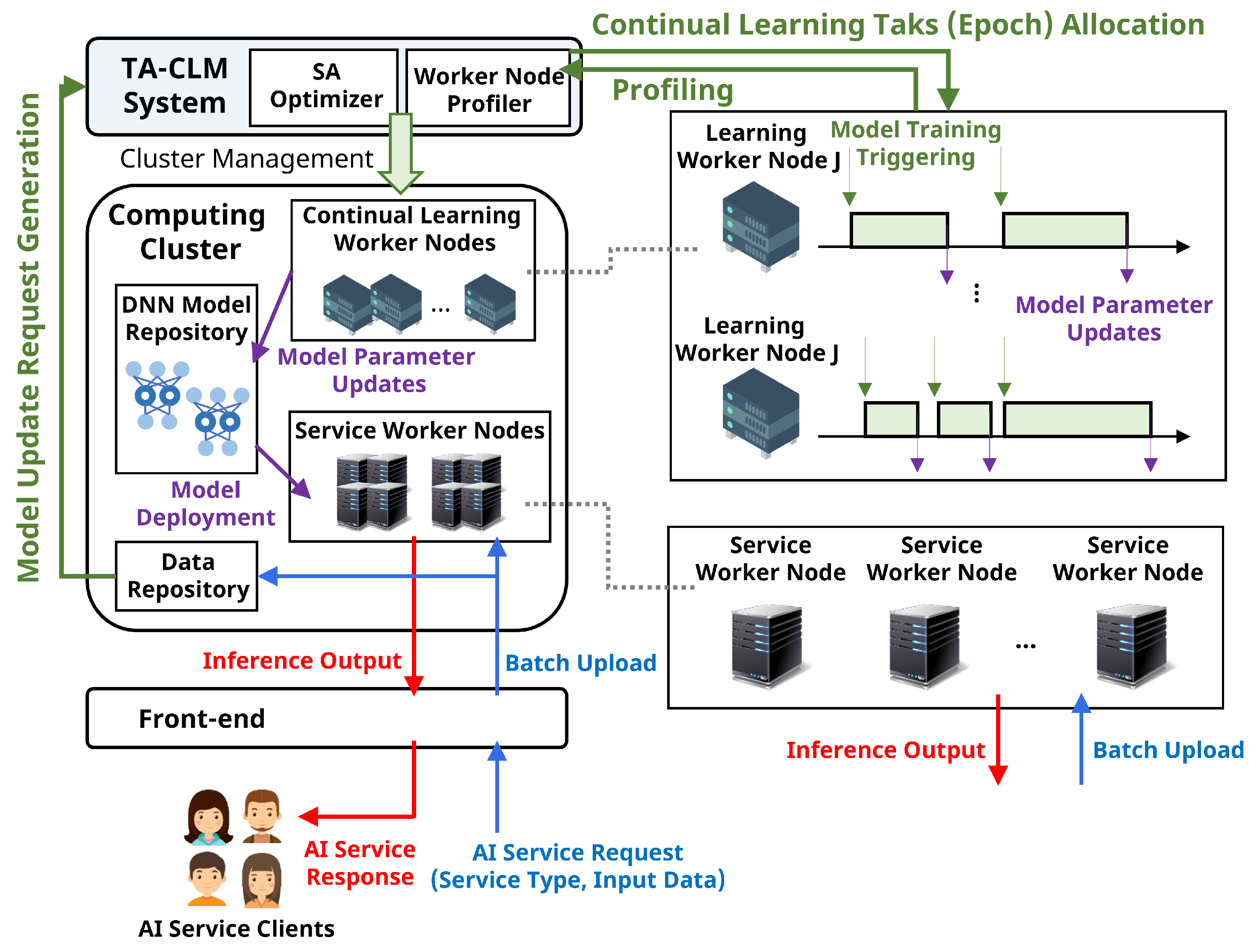
Figure 2.
Model update latency for continual learning.

Figure 3.
Penalty cost curves for model update latency bound violations.

Figure 4.
Allocation of two sequential tasks with overlap.

Figure 5.
Energy consumption for 200 epochs of 4 node types and 4 DNN models in pairs.

Figure 6.
Model update latency and bound violation ratio for scenarios 1, 2, and 3.

Figure 7.
Energy consumption and non-violated requests per Unit of Energy (UoE) for Scenarios 1, 2, and 3.
Figure 7.
Energy consumption and non-violated requests per Unit of Energy (UoE) for Scenarios 1, 2, and 3.


Table 1.
Notations in the formulation.
| Notation | Description |
|---|---|
| Decision variable for task allocation of i-th request onto j-th worker node at time slot g. | |
| Auxiliary decision variable. | |
| , | Model coefficients to predict . |
| Data sample size of i-th request. | |
| Arrival time of i-th request. | |
| DNN model update time for i-th request on j-th worker node. | |
| Power consumption for training DNN model on j-th worker node. | |
| DNN model update latency of i-th request on j-th worker node at triggering time slot g. | |
| , , | (Indicator, linear, exponential) cost metrics for violation of model update latency bound. |
| Model update latency bound for i-th request. | |
| Energy consumption for i-th request on j-th worker node. | |
| Energy consumption cost for . | |
| Violation cost of h-th constraint set. |
Table 2.
Worker node specifications.
| Node1 (Laptop) | Node2 | Node3 | Node4 | |
|---|---|---|---|---|
| CPU | i7-9750H | i7-4790 | i5-11400F | i9-10900K |
| Board | MS-16W1 | B85M Pro4 | B560M-A | Z490 Ext4 |
| MEM | DDR4 16 GB | DDR3 32GB | DDR4 32 GB | DDR4 64 GB |
| GPU | RTX2060m (6 GB) | RTX2060 (6 GB) | RTX3060 (12 GB) | RTX3090 (24 GB) |
| Disk | KINGSTON 512 GB | SSD850 256 GB | WD SN350 1 TB | SSD970 1 TB |
Table 3.
Power consumption and DNN model training time (for 1 epoch).
| Node1 (Laptop) | Node2 | Node3 | Node4 | ||
|---|---|---|---|---|---|
| VGG16 | Power (W) | 43 | 143 | 131 | 338 |
| Time (s) | 74.5 | 39.5 | 36.5 | 20.09 | |
| MobileNet | Power (W) | 41 | 140 | 133 | 343 |
| Time (s) | 62.1 | 31.1 | 21.6 | 16.06 | |
| ShuffleNet | Power (W) | 39 | 125 | 132 | 301 |
| Time (s) | 139.6 | 86.2 | 50.8 | 43.5 | |
| Attention56 | Power (W) | 47 | 156 | 146 | 262 |
| Time (s) | 232.7 | 129.5 | 100.3 | 83.9 | |
Disclaimer/Publisher’s Note: The statements, opinions and data contained in all publications are solely those of the individual author(s) and contributor(s) and not of MDPI and/or the editor(s). MDPI and/or the editor(s) disclaim responsibility for any injury to people or property resulting from any ideas, methods, instructions or products referred to in the content. |
© 2023 by the author. Licensee MDPI, Basel, Switzerland. This article is an open access article distributed under the terms and conditions of the Creative Commons Attribution (CC BY) license (https://creativecommons.org/licenses/by/4.0/).
Share and Cite
MDPI and ACS Style
Kang, D.-K. Energy-Efficient and Timeliness-Aware Continual Learning Management System. Energies 2023, 16, 8018. https://doi.org/10.3390/en16248018
AMA Style
Kang D-K. Energy-Efficient and Timeliness-Aware Continual Learning Management System. Energies. 2023; 16(24):8018. https://doi.org/10.3390/en16248018
Chicago/Turabian StyleKang, Dong-Ki. 2023. "Energy-Efficient and Timeliness-Aware Continual Learning Management System" Energies 16, no. 24: 8018. https://doi.org/10.3390/en16248018
Note that from the first issue of 2016, this journal uses article numbers instead of page numbers. See further details here.