Heat Transfer Mechanism of Heat–Cold Alternate Extraction in a Shallow Geothermal Buried Pipe System under Multiple Heat Exchanger Groups

Abstract

Shallow geothermal energy usually uses underground buried pipes to achieve the purpose of extracting heat while storing cold in winter and extracting cold while storing heat in summer. However, the heat transfer mechanism under the alternate operation of heat–cold extraction in winter and summer under multiple heat exchanger groups is still worth studying. Based on the constructed flow and heat transfer model in pipelines and reservoirs, this study first analyzes the temperature field evolution of a shallow buried pipe system (SBPS) under the alternate operation of heat–cold extraction, and then discusses the heat transfer performance under different pipeline flow rates, pipeline wall thermal conductivity, heat injection durations, numbers of heat exchanger groups, and flows of underground fluid. The results show that the continuous alternating process of heat–cold extraction has a promoting effect on the temperature increase or decrease in the next operating cycle due to the low- or high-temperature zone produced in the previous operating cycle. As the number of multiple heat exchanger groups increases, the heat transfer efficiency of the SBPS significantly improves. With a rise in the groundwater flow velocity, the heat transfer efficiency first decreases and then increases.

1. Introduction

At present, global warming and carbon emissions have become shared problems faced by mankind. The application of geothermal energy, especially shallow geothermal energy, is more in line with the development needs of energy saving and carbon reduction. It has significant advantages such as a low cost, high efficiency, winter heating and summer cooling, and a long service duration [1]. Shallow geothermal energy is mainly extracted using buried pipes [2,3,4]. At present, scholars have conducted a lot of research on the heat transfer mechanism and heat transfer efficiency of single buried pipe groups [5,6]. However, for more efficient heat exchange, multiple sets of buried pipe heat exchangers are usually laid underground [7,8], but there is still lack of research on the winter–summer cycle process with multiple heat exchanger groups. Therefore, it is of significance to explore the heat transfer mechanism of the whole heat–cold alternate process of a shallow buried pipe system (SBPS) in winter and summer, and discuss the influence degree of each development parameter on the heat transfer performance under the condition of multiple heat exchanger groups, which can provide support for the scientific optimization of SBPSs in shallow geothermal system development.

Some scholars have studied the influence of the buried pipe characteristics on the heat transfer performance of SBPSs [9]. Kerme et al. [10] simulated the heat transfer of single U-tube and double U-tube underground heat exchangers and found that under the condition of heat extraction, the heat transfer efficiency of a double U-tube underground heat exchanger is about 40% higher than that of a single U-tube. Jahanbin [11] compared the thermal comportment of an elliptical single U-tube with a typical GHE and investigated the influencing factors of the novel elliptical tube. The results showed that the proposed novel vertical GHE with an elliptical U-tube is promising for enhancing the thermal performance. Chen et al. [12] analyzed the heat exchange efficiency of a buried pipe energy pile group and found that the inlet temperature and flow rate of the circulating medium had a great influence on its heat transfer performance. Cai [13] investigated the influencing factors for the heat transfer capacity of a vertical ground heat exchanger. The results showed that the initial average temperature of the soil and the temperature difference in the heat transfer medium are positively correlated with the heat transfer capacity of the heat exchanger. Li et al. [14] numerically simulated the heat transfer process of shallow-buried horizontal and deep-buried vertical U-tube systems. It was found that the outlet temperature of the shallow-buried horizontal tube system was significantly affected by the inlet velocity and temperature, while the outlet temperature in the deep-buried vertical U-tube system varied greatly with the operating conditions. Meanwhile, the short intermittent operation scheme reduced the soil temperature fluctuation around the pipeline, which is conducive to the thermal recovery of the soil around the U-tube. Chen et al. [15] simulated the heat transfer performance of a double U-shape buried heat exchanger (BHE) and an enhanced coaxial buried heat exchanger (BHE) with intermittent spiral ring fins by establishing three-dimensional geometric models. The results showed that the heat transfer performance of the enhanced coaxial BHE was 1.45 times better than that of the common BHE. Based on numerical simulation, the optimal injection flow rate and depth of buried heat exchangers with different pipe diameters were determined by Hong et al. [16]. They found that the energy consumption of the heat exchange system in summer increased at first and then decreased with an increase in drilling depth. Harris et al. [17] conducted a transient performance comparation of coaxial and u-tube borehole heat exchangers, and the results show that the coaxial heat exchanger outperforms the u-tube heat exchanger at the early stages. Wang et al. [18] studied the influence of the pipeline flow rate on the properties of the soil around the pipeline. The results show that the soil properties are closely related to the pipeline flow rate, and the increase in the cycle number and flow rate can be attributed to the gradual softening and grooving effect of the soil until it is relatively stable. Jahanbin et al. [19] explored the performance of U-tube borehole heat exchangers adopting heat-carrying nanofluids, and the results show that all nanofluids showed a higher rate of heat transfer enhancement than pressure drop.

Some scholars have studied the influence of the formation characteristics on the heat transfer performance of SBPSs. Li et al. [20] analyzed the influence of the geological conditions and buried pipe form on the SBPS heat transfer performance by using field experimental data on the geotechnical thermal response of 35 heat exchange holes in Beijing. The results show that the geological conditions have a significant effect on the SBPS heat transfer performance: the initial average temperature of the formation changing by 1 °C will induce the heat transfer capacity to vary by about 8%. The heat transfer capacity of the buried pipe system in the tight layer is 35% higher than that in the loose layer. Ye et al. [21] used a Test Protocol Hot Disk TPS 2500 S thermal constant analyzer to carry out thermal parameter experiments and discussed the variation in the thermal parameters of loess with different water contents and dry densities. It was found that when the water content of the loess samples was constant, the greater dry density increased the thermal conductivity, specific heat capacity, and thermal diffusion coefficient, and the thermal conductivity and specific heat capacity of the loess samples increased linearly with an increase in water content. When the water content was low, the thermal diffusion coefficient increased with the increase in water content. When the water content reached a certain value, the thermal diffusion coefficient decreased with the increase in water content. Florides et al. [22] explored the heat performance of U-tube ground heat exchangers in multiple layer substrates, and the results showed that the thermal energy in the soil disperses more easily in the top layers. Du et al. [23] established a three-dimensional coupling numerical model of unsteady groundwater seepage and heat transfer and found it was an effective way to optimize and determine the sustainable development and utilization scheme of a shallow geothermal energy ground source heat pump. Yue et al. [24] used TOUGH2 software (v2017) to predict the distribution of soil temperature and found that the distribution of temperature field was significantly affected by the groundwater flow rate. Anthony et al. [25] evaluated the heat transfer performance of SBPS by computational fluid dynamics simulation. The results showed that the permeability of soil, the location of the irrigation pipeline, and the water content of soil greatly affected the water pattern of SBPS, thus affecting the system efficiency. Wang et al. [26] investigated the buried pipes heat transfer in fractured rock mass by statistical analysis of the outcrop cracks characteristics based on the coupled model of water flow, convective heat transfer, and the cubic law.

Some scholars have studied the influence of backfill materials on the heat transfer performance of shallow buried pipe systems. Fei et al. [27] used the comprehensive scoring method to test the fluidity, thermal conductivity, and compressive strength of backfill materials. And the influence of waste steel slag and graphite as composite additives on the comprehensive performance of backfill materials for buried pipes was studied. It was found that the addition of waste steel slag was beneficial to improve the construction performance of backfill materials The addition of waste steel slag led to a decrease in the heat transfer performance of the backfill material, but the maximum thermal conductivity loss of 6.5% can be compensated by adding graphite. The addition of graphite had little effect on the mechanical properties of backfill materials, but the compressive strength could be increased by 97.5% by adding waste steel slag. Xu et al. [28] proposed to use the waste steel slag–clay mixture as the backfill material for ground source heat pumps and investigated the heat transfer rule of the backfill material from the micro-scope perspective. Song et al. [29] studied the influence of the thermal conductivity of backfill materials on the heat transfer efficiency in summer conditions by establishing the heat transfer characterization model of double vertical U-tubes. It was found that the thermal conductivity of backfill materials had a certain influence on the heat transfer efficiency of the buried pipe system, but the improvement in the heat transfer capacity of buried pipe was limited. Mascarin et al. [30] determined the selection of backfill grout for SBPS through thermo-physical laboratory analysis and proposed the grout criteria of working time, water bleeding target, volumetric shrinkage, and thermal conductivity.

In addition, buried pipe heat exchange systems also have wide applications in garbage treatment, tunnel heat extraction, ground snow melting, shallow heat storage, and other areas [31,32,33]. Chen [34] studied the heating effect and heat transfer performance inside the landfill. It was found that the temperature of the landfill in the dense buried pipe changed significantly, and the heat transfer upward was more than downward. In summer, the heat exchange capacity of the buried pipe increased first and then decreased. Wei et al. [35] analyzed the influence of inlet/outlet temperature and thermal-induced stress on the extraction of shallow geothermal energy by an energy tunnel. It was found that the heat transfer efficiency was positively correlated with the inlet temperature and flow rate, and negatively correlated with pipeline spacing. Carlos et al. [36] proposed an experimental solar-assisted ground source heat pump (SAGSHP) system for home heating applications and demonstrated that the system can meet the space heating needs of buildings in winter. Shi et al. [37] investigated the influence of the operation parameters and well-layout parameters for the aquifer thermal energy storage system, and the results showed that the optimization scheme can expand the thermal storage volume and reduce the heat loss. Harjunowibowo et al. [38] explored the performance of shallow seasonal soil energy storage heat pumps in greenhouses. By installing thermal insulation materials, it was found that the seasonal coefficient of performance (COP) of the heat pump varies between 1.48 and 2.97 and 1.20 and 3.345 for heating and cooling, respectively. Nagare et al. [39] proposed a simple and effective method to simulate the ground temperature of buried pipelines under the influence of snow and freeze–thaw conditions and verified the method through engineering examples. The results showed that the method can be used to better understand the influence of high-temperature pipelines on the underground thermal state, helping to design the ground temperature detection program, and successfully identified the pipeline insulation damage.

All in all, it can be found that the current research studies have mainly focused on the buried pipe forms, soil geological conditions, backfill materials, and the heat transfer of a single heat transfer exchanger. For more efficient heat exchange, multiple sets of buried pipe heat exchangers are usually laid underground, and there is still a lack of winter–summer cycle process research under the multiple heat exchanger groups. In this research, based on the constructed flow and heat transfer model in the pipeline and the coupled model of heat transfer between the pipeline and reservoir, firstly, the heat transfer mechanism of the whole heat–cold alternate process of the SBPS with multiple heat exchanger groups is explored, then the influence of buried pipe characteristics and development parameters on heat transfer performance are investigated. Through this research, the results can provide support for the optimization design of the buried pipe heat exchanger system.

2. Numerical Model

The heat extraction from the shallow buried geothermal system involves the fluid flow and heat transfer in the pipeline, the fluid flow and heat transfer in the shallow reservoir, and the heat transfer between the reservoir and pipeline. For the study of flow and heat transfer in pipes with a short distance, pipes are usually described as two-dimensional or three-dimensional geometries containing internal grids [40,41]. However, in the study of the heat transfer of a buried pipe geothermal system, pipes have a large length and complex structures. Therefore, for the efficient construction of multiple heat transfer groups, the built-in non-isothermal pipeline flow module in COMSOL is used.

2.1. Flow Equations in the Pipeline

The continuity and momentum equations below describe the stationary flow inside the pipe system:

$$\begin{array}{l}\nabla \cdot (A\rho u)=0\\ 0=-\nabla p-f_D\frac{\rho }{2d_h}u\left|u\right|+F\end{array}$$

(1)

where,

$A$—Pipeline cross-sectional area, m²;

$\rho$—Density, kg/m³;

$u$—Fluid velocity, m/s;

$p$—Pressure, N/m²;

$F$—Volume force, such as gravity, N/m³.

The right side of Formula (1) describes the pressure drop caused by internal viscous shear. This term includes the Darcy friction coefficient f_D, which is a function of the Reynolds number and surface roughness divided by the hydraulic tube diameter (e/dh).

The non-isothermal pipe flow interface in COMSOL provides a built-in expression library of the Darcy friction coefficient f_D, which is valid for laminar flow, turbulent flow, and the transitional region in between [42].

The Churchill relationship is:

$$f_D=8{\left[{\left(\frac{8}{\mathrm{Re}}\right)}^{12}+{\left(A+B\right)}^{-1.5}\right]}^{1/12}$$

(2)

where

$$\begin{array}{l}A={\left[-2.457\ln \left({\left(\frac{7}{\mathrm{Re}}\right)}^{0.9}+0.27(e/d)\right)\right]}^{16}\\ B={\left(\frac{37530}{\mathrm{Re}}\right)}^{16}\end{array}$$

As seen in the above equation, the friction coefficient is a function of the surface roughness divided by the pipe diameter. Surface roughness data can be selected from the predefined list in the ‘Pipe Features‘ function. The Churchill equation is also a function of fluid properties, through the Reynolds number:

$$\mathrm{Re}=\frac{pud}{\mu }$$

The physical properties of the fluid can be obtained directly from the COMSOL6.1‘s built-in material library. Formula (2) shows that for a low Reynolds number (laminar flow), the friction coefficient is 64/Re, and for a very high Reynolds number, the friction coefficient is independent of Re.

2.2. Heat Transfer Equations in the Pipeline

The continuity and momentum equations below describe the stationary flow inside the pipe system:

$$pA{C}_{\rho }u·\nabla T=\nabla ·Ak\nabla T+{\mathrm{f}}_D\frac{p}{2d_h}{\left|u\right|}^3+Q_{wall}$$

(3)

Above, $A$ (m²) is the cross section area of the pipe, $\rho$ kg/m³) is the density, $u$ (m/s) is the fluid velocity, and $p$ (N/m²) is the pressure, and $F$ (N/m³) is a volume force, like gravity.

$$Q_{wall}=\mathrm{hZ}({\mathrm{T}}_{\mathrm{ext}}-T)$$

(4)

where Z (m) is the wetted perimeter of the pipe, h (W/(m²·K)) is an overall heat transfer coefficient, and Text (K) the external temperature outside of the pipe. The overall heat transfer coefficient includes contribution from internal film resistance, wall resistance, and external film resistance.

For a circular pipe, under the assumption that the heat transfer through the wall is quasi static and that the temperature is equal around the circumference of the pipe, an effective hZ in Equation (4) is given by

$${\left(\mathrm{h}Z\right)}_{eff}=\frac{2\pi }{\frac{1}{{\mathrm{r}}_0{\mathrm{h}}_{\mathrm{int}}}+\frac{1}{{\mathrm{r}}_N{h}_{ext}}+{\displaystyle \sum _{n=1}^N\left[\frac{\ln \left(\frac{r_n}{r_{n-1}}\right)}{k_n}\right]}}$$

(5)

where $r_n$ is the outer radius of wall n, hint and $h_{ext}$ are the film heat transfer coefficients on the inside and outside of the tube, and $k_n$ is the thermal conductivity of wall $n$. The film resistance inside the pipe is given by:

$$h_{\mathrm{int}}=N{u}_{\mathrm{int}}\frac{k_{water}}{d}$$

(6)

The internal Nusselt number is taken as 3.66 for the laminar flow regime and for the turbulent flow regime, the Gnielinski correlation for internal pipe flow is used:

$$N_{\mathrm{int}}=\frac{\left(f_D/8\right)\left(\mathrm{Re}-1000\right)\mathrm{Pr}}{1+\sqrt{12.7\left({\mathrm{Pr}}^{2/3}-1\right)}}$$

(7)

The external film resistance around the pipe is:

$$h_{ext}=N{u}_{ext}\frac{k_{water}}{d}$$

(8)

A slow current is present in the pond. For external forced convection around a pipe, COMSOL uses the Churchill and Bernstein relation for Nu, valid for all Re and for Pr > 0.2:

$$N{u}_{\mathrm{ext}}=0.3+\frac{0.62{\mathrm{Re}}^{1/2}{\mathrm{Pr}}^{1/3}}{{\left[1+{\left(0.4/\mathrm{Pr}\right)}^{2/3}\right]}^{1/4}}{\left[1+{\left(\mathrm{Re}/282000\right)}^{5/8}\right]}^{4/5}$$

(9)

where Pr = Cpμ/k.

2.3. Flow Equations in the Reservoir

$$\rho S\frac{\partial \mathrm{p}}{\partial t}+\nabla \cdot (\rho v)=Q_m$$

(10)

The flow of liquid in the porous elastic medium of the matrix is depicted by the mass balance equation in Equation (10) [43,44], where ρ is the matrix density, kg/m³; S is the storage coefficient of matrix rock; t is the development time; Qm is the term of seepage source, kg/(m³·s); ν is water flow velocity in matrix rock, m/s. The liquid flow in the matrix follows Darcy’s law:

$$v=-\frac{k}{\mu }\nabla \cdot p$$

(11)

where $k$ is the matrix permeability, m²; $\mu$ is the hydrodynamic viscosity, Pa·s; $p$ is the pressure, Pa.

2.4. Heat Transfer Equations in the Reservoir

$${\left(\rho C\right)}_M\frac{\partial T}{\partial t}+{\rho }_l{C}_l\left(T_0+T\right)\frac{k}{\mu }\nabla p={\lambda }_M{\nabla }^{2}T$$

(12)

The heat transfer in the porous medium of the reservoir is described in Equation (12), where ${\lambda }_M={\lambda }_s\left(1-\varphi \right)+{\lambda }_l\varphi$, and ${\lambda }_s$ and ${\lambda }_l$ respectively represent the thermal conductivity coefficient of the matrix and the fluid (W/(m·K)); $T_0$ is the reference temperature under the zero stress state (K); and the heat capacity of the porous media containing the fluid can be described as ${\left(\rho C\right)}_M={\rho }_s{C}_s\left(1-\varphi \right)+{\rho }_l{C}_l\varphi$ (KJ·m³·K⁻¹).

3. Simulation Model Construction

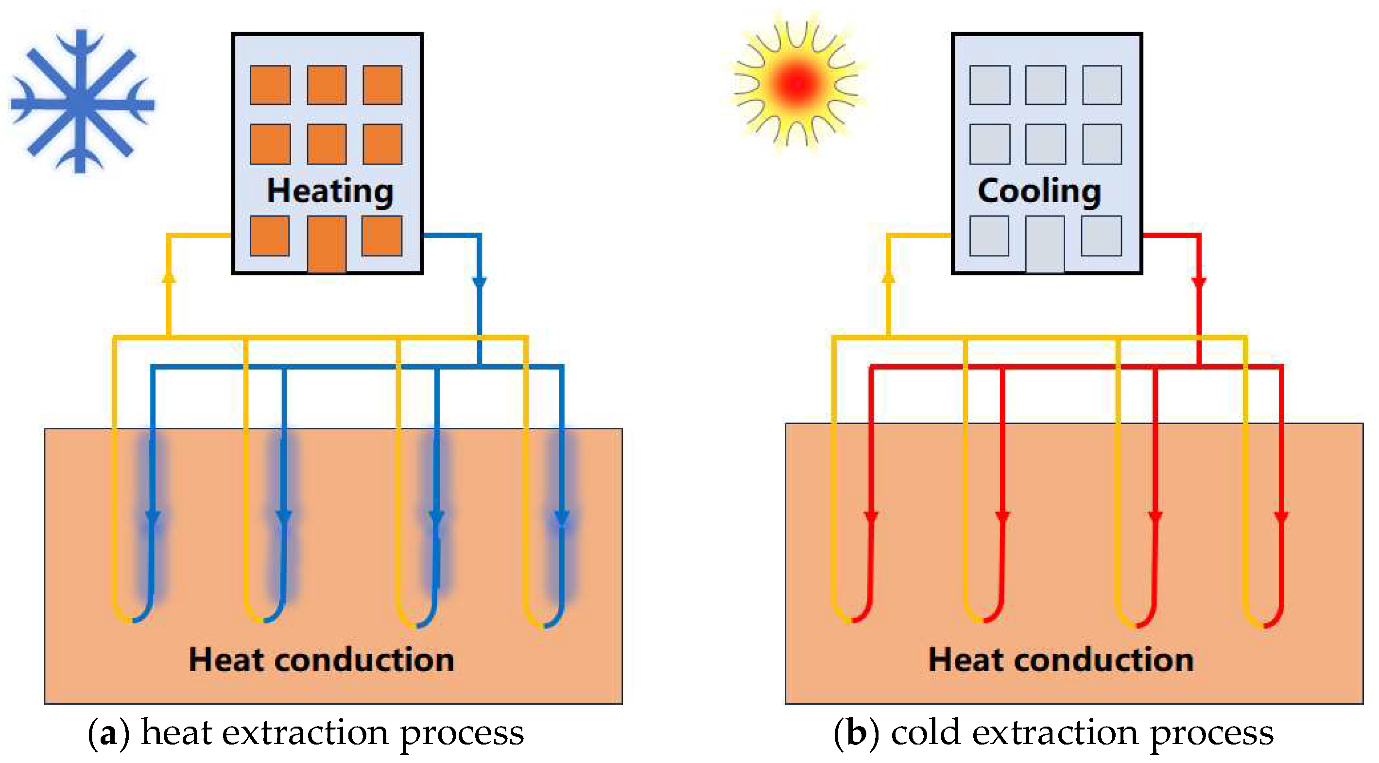
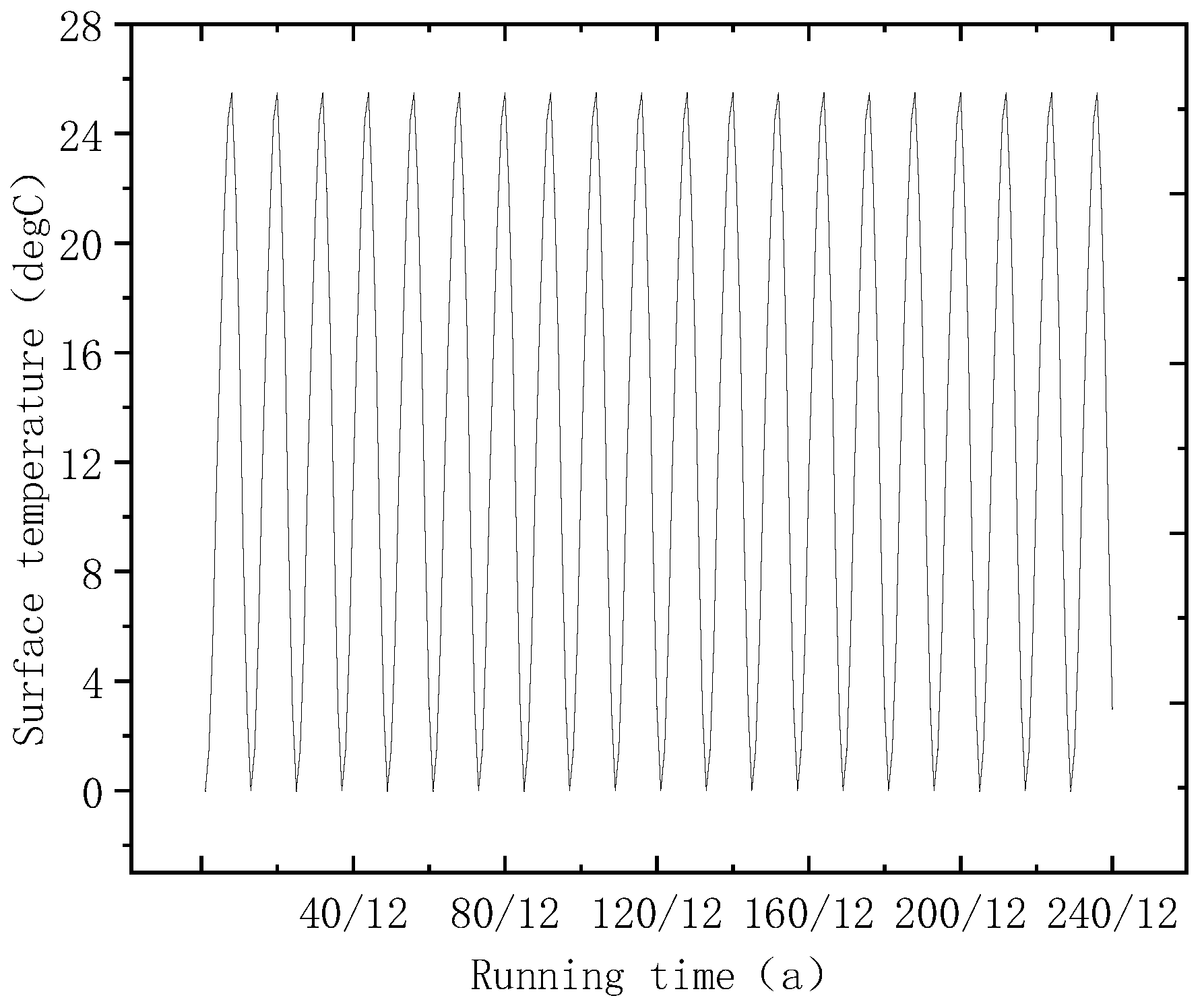
3.1. Heat Transfer Principle of the Shallow Buried Pipe

Shallow geothermal energy usually uses underground buried pipes to extract energy and can achieve the purpose of taking heat and storing cold in winter and taking cold and storing heat in summer. The ground source heat pump system uses the soil as the cold source in summer and the heat source in winter, as shown in Figure 1. The borehole heat exchanger is buried underground by drilling and backfilling to realize the heat exchange between the system and the underground soil. There are various forms of underground buried pipes. In this study, U-shaped buried pipes are used for the heat exchangers.

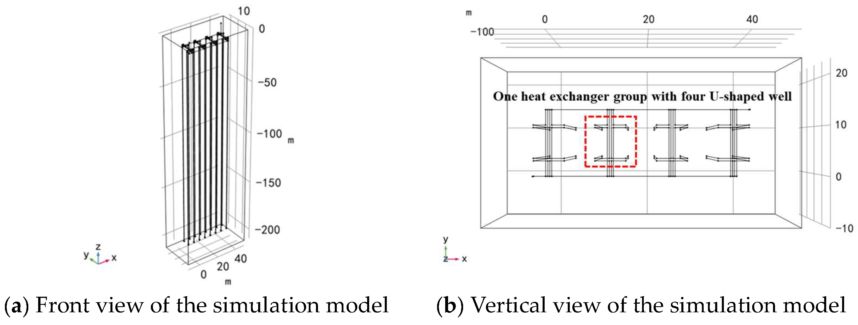
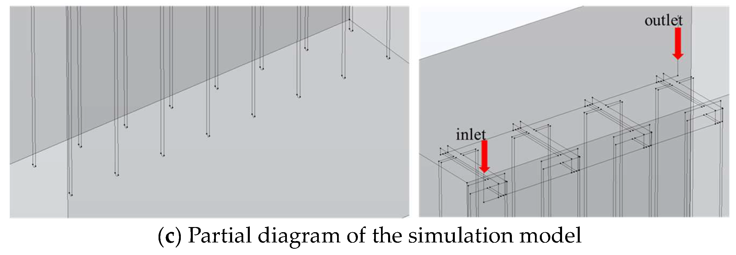
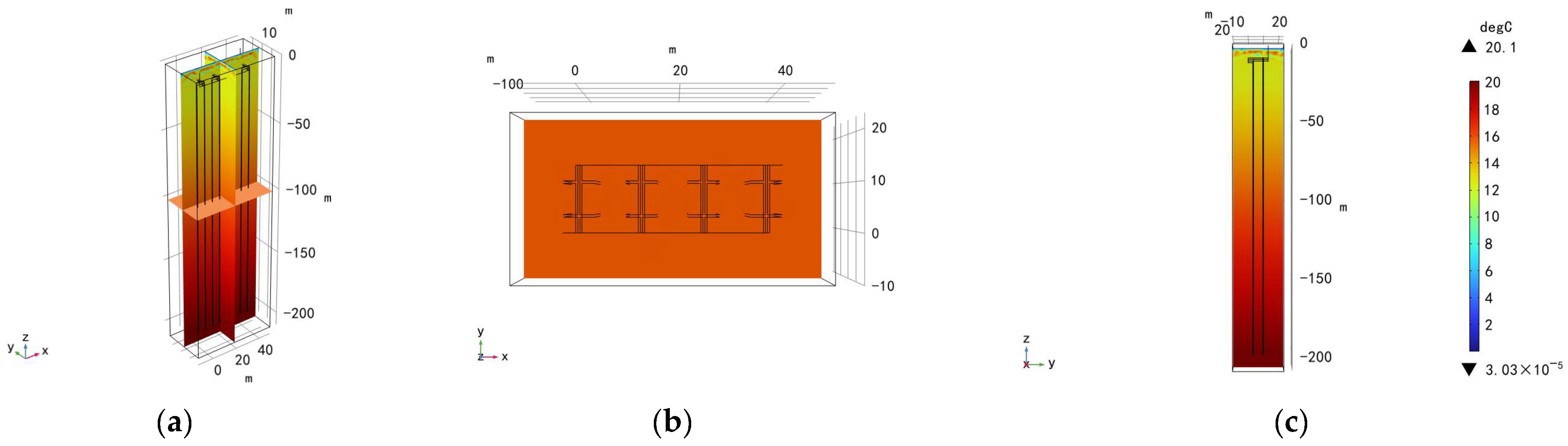
3.2. Model Establishment

The model includes the soil layer and the multiple U-shaped buried pipe heat exchangers, and four U-shaped tubes are organized as one heat exchanger group, the distance between each U-shaped buried pipe is 6 m, and the length of each U-shaped buried pipe is 200 m, as shown in Figure 2. In Figure 2c, the circulating medium enters the system from the inlet, flows through the circulating pipe into each U-shaped tube for heat exchange with the soil layer, and then flows out through the outlet. And the geometric dimensions of the model include the height of 210 m, length of 62 m, and width of 33 m.

To highlight the impact of SBPS development on the reservoir temperature during the alternating process of heat and cold extraction, the climate characteristics that are not obvious in spring and autumn (such as Qingdao) are selected in this research. The inlet temperature is set to 30 °C from April to September (simulating the cold extraction process in summer) and 5 °C from October to March (simulating the heat extraction process in winter) [9], as shown in Figure 3. The atmospheric temperature setting is shown in Figure 4, which considers the temperature variation with the change in seasons. Taking the year as the time unit, 1/12 represents one mouth. And the heat cold alternate extraction period is set to 20 years; the numerical simulation time interval is set to 0.01 year. And the simulations are conducted by the multi-physics software COMSOL. The simulation parameters are shown in

Table 1. Simulation parameters [9].

Project	Value	Unit
Height of the geometric model	210	m
Length of the geometric model	62	m
Width of the geometric model	33	m
Pipeline diameter	36	mm
Pipeline flow rate	1	l/s
Temperature gradient	0.027	°C/m
Formation thermal conductivity	1.5	W/(m·k)
Formation permeability	10 × 10−12	m2
Thermal conductivity of pipeline	10	w/(m·k)
Pipeline wall thickness	0.005	m
Darcy friction coefficient	1.5 × 10−3	mm
Number of U-shaped tube heat exchanger groups	4	group
Injection temperature in winter	5	°C
Injection temperature in summer	30	°C
Length of U-shaped buried well	200	m
Distance between each U-shaped buried pipe	6	m
Pipeline diameter	36	mm

. For the definition of the initial reservoir temperature, the underground constant temperature zone is set at the depth of −20 m with the temperature of 15.1 °C. And the boundary condition of the upper surface is set as the temperature boundary with the variation atmospheric temperature, which transfers the heat above the constant temperature zone by thermal diffusivity. Then, the reservoir temperature gradient below the constant temperature zone is set as 0.027 °C/m. The thermal conductivity of the reservoir is 1.5 W/(m·k), and the permeability of the reservoir is 10 × 10⁻¹² m².

4. The Temperature Field Evolution during the Heat–Cold Alternate Extraction

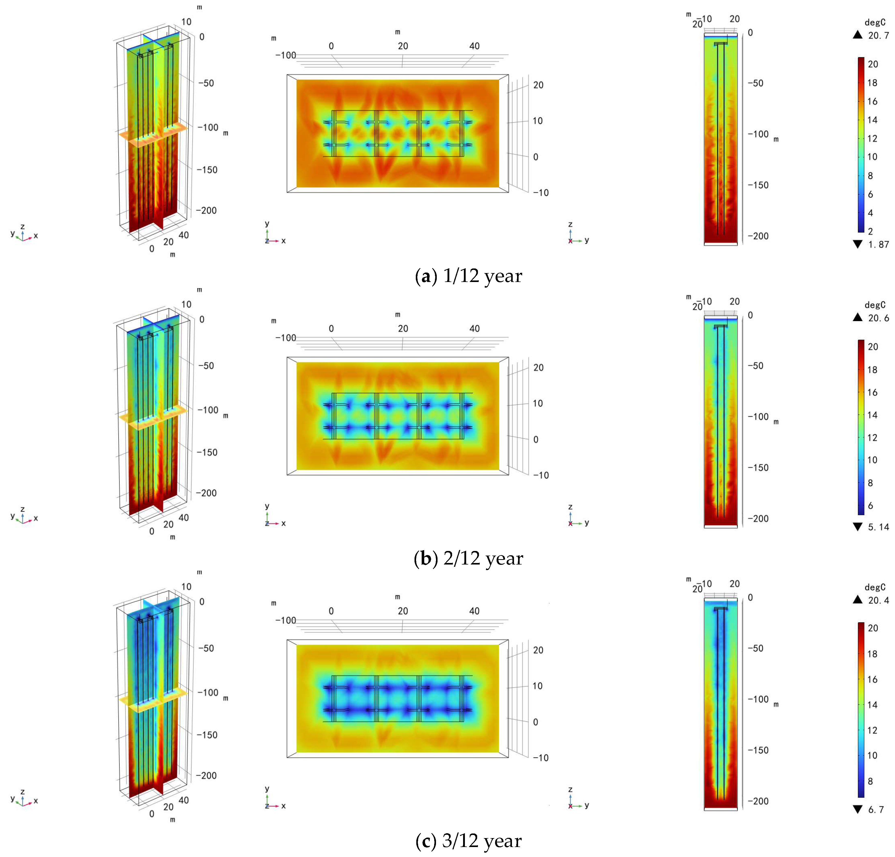
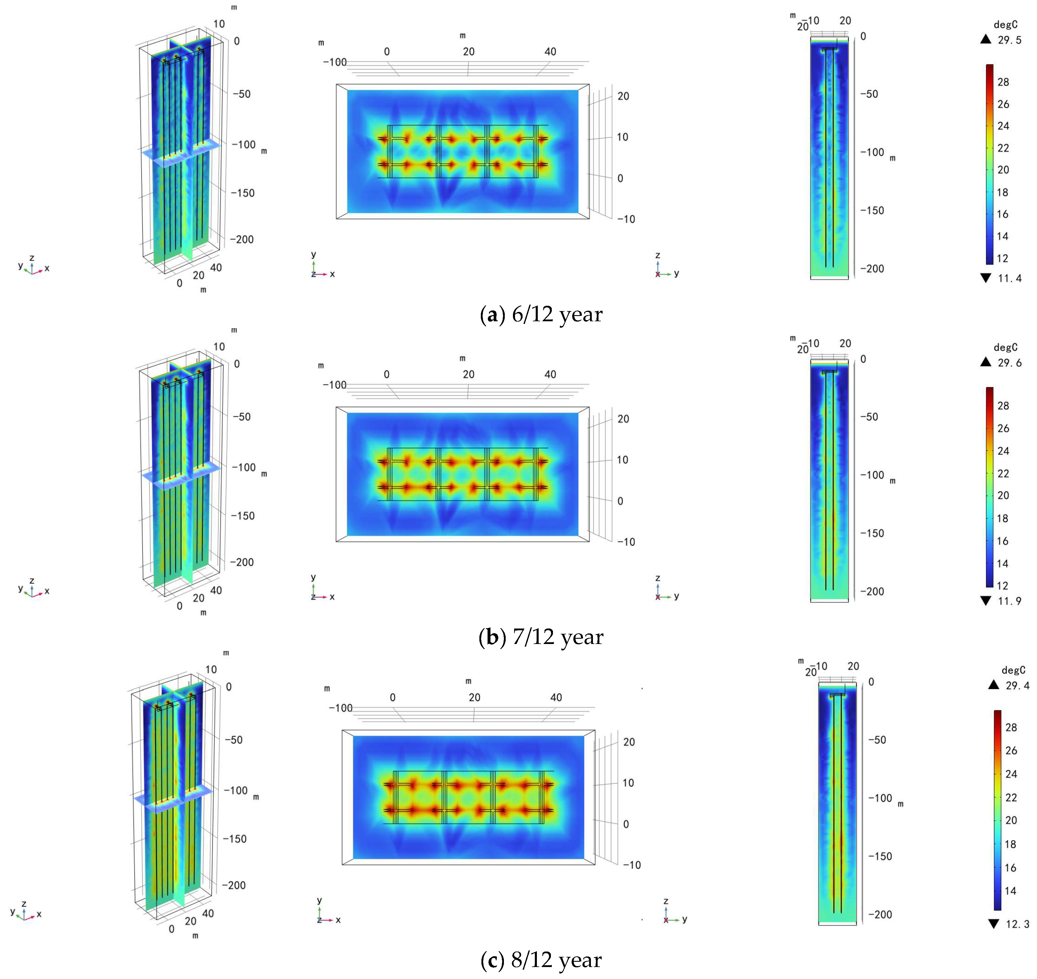
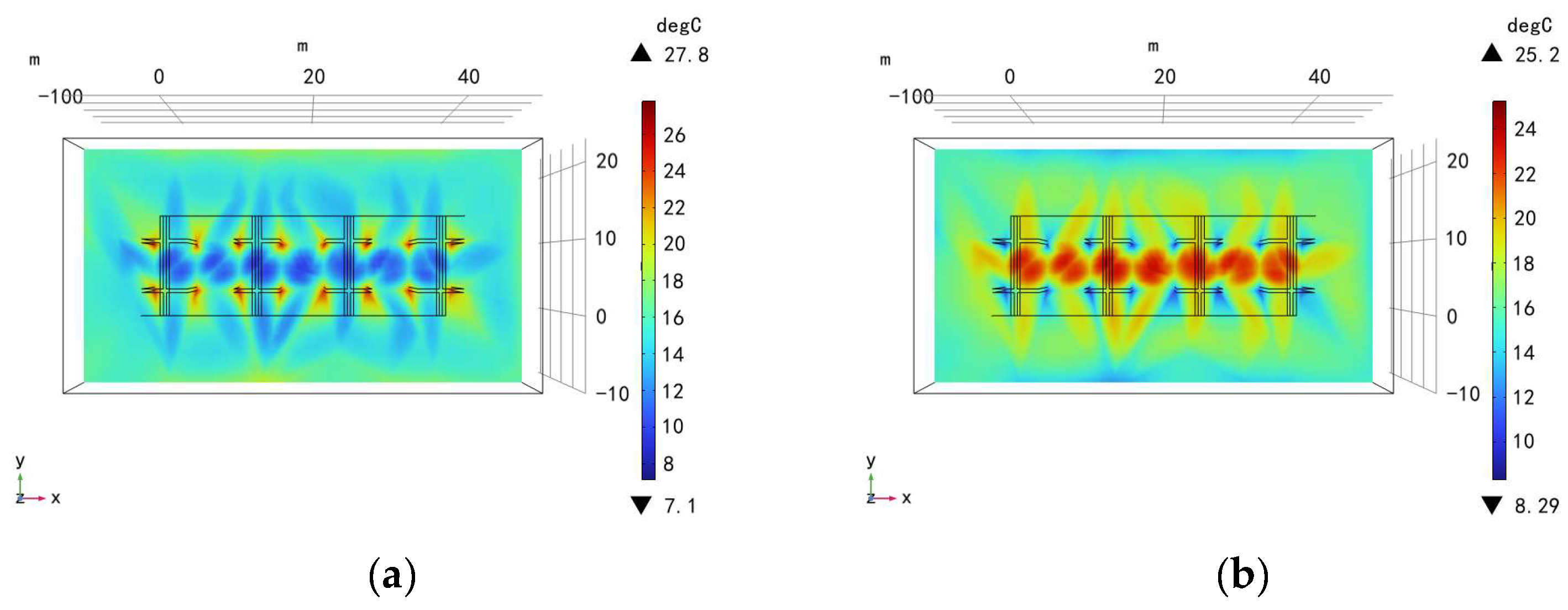
4.1. Temperature Evolution in the Reservoir

The heat–cold alternate extraction process of a shallow buried pipe geothermal system must disturb the evolution of the rock temperature field. The initial temperature field in the reservoir is shown in Figure 5. In the vertical direction, the maximum temperature is 20.1 °C, and the minimum temperature is 13.1 °C. And the XY cross-section of −100 m buried depth and the YZ cross-section in the middle of the 3D model are taken to study the temperature field change in the shallow buried pipe system (SBPS).

After the completion of the buried geothermal system in the shallow geothermal reservoir, the heat extraction process will be carried out in winter by the injection of cold fluid. In this simulation, the fluid with a temperature of 5 °C is injected into the buried pipe, then the cold fluid will flow and exchange heat in the pipelines. As shown in Figure 6, the initial heat in the shallow reservoir is extracted by the U-shaped tube heat exchangers after heat exchange, which creates a low-temperature area around each U-shaped tube. As the heat extraction lasts, the low-temperature area gradually diffuses outward. After a period of operation, the continuous low-temperature area surrounding the SBPS is formed. From the longitudinal perspective (Figure 6c), the lowest temperature appears in the upper reservoir.

With the season change, when the environmental temperature rises, it is necessary to use the SBPS for cooling in summer by the injection of hot fluid, and the injection temperature of hot fluid in this process is 30 °C. Due to the use of a shallow reservoir for heat extraction by cold injection in the previous stage, a certain low-temperature area has been formed near the pipeline system. As shown in Figure 7, when high-temperature fluid is injected into the pipeline, the original low-temperature center gradually becomes the high-temperature center. From the longitudinal direction (Figure 7c), the highest temperature appears in the lower part of the reservoir.

During the conversion process of heat extraction to cold extraction (that is the beginning of the summer cooling stage after the winter heating stage), the low-temperature area created in the formation during the previous heat extraction cycle by the cold fluid injection can promote a decrease in outlet temperature during the summer cooling process (Figure 8a). Similarly, during the conversion of cold extraction to heat extraction, the previous cold extraction cycle by the hot fluid injection can promote the increase in outlet temperature during the winter heating process (Figure 8b).

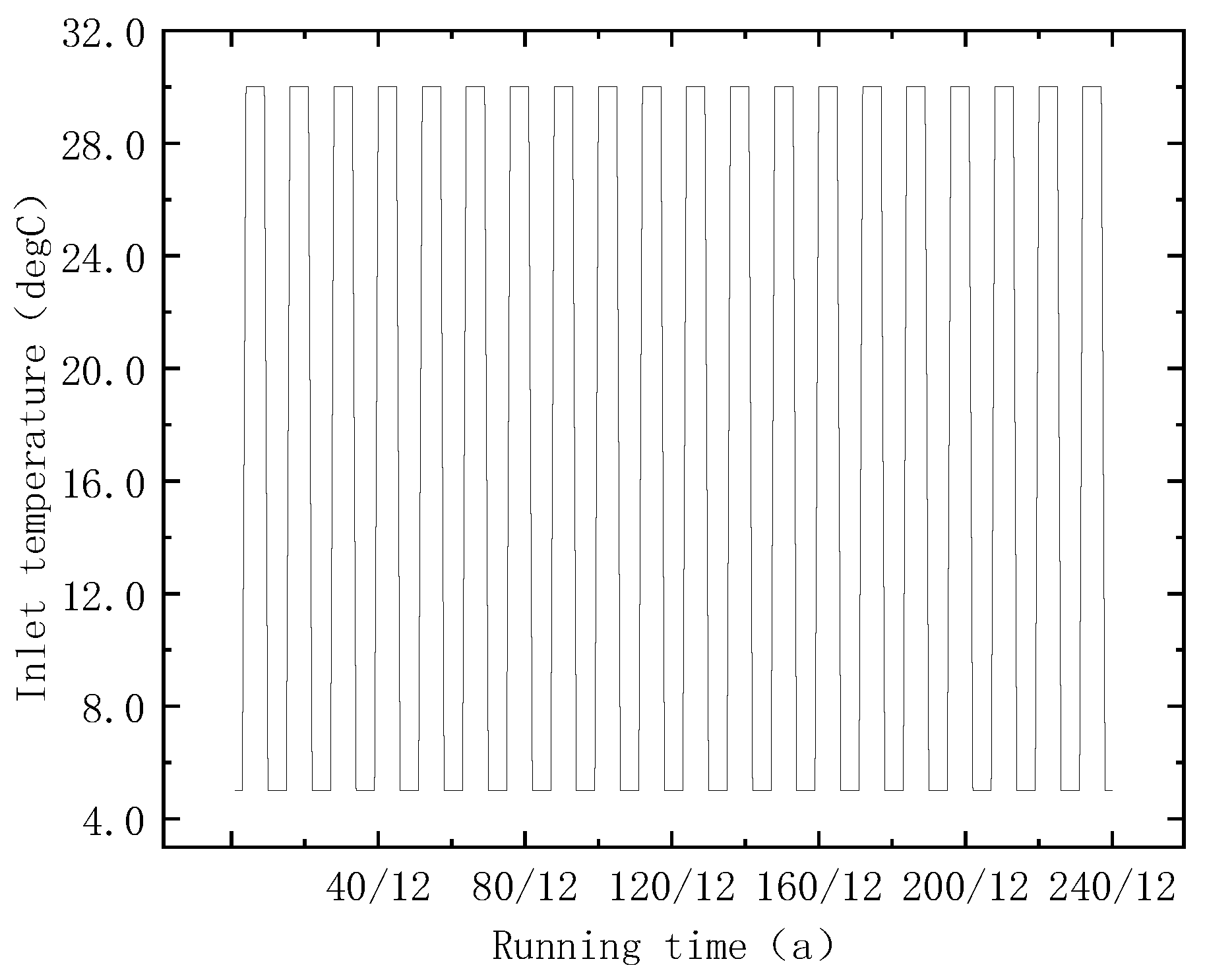
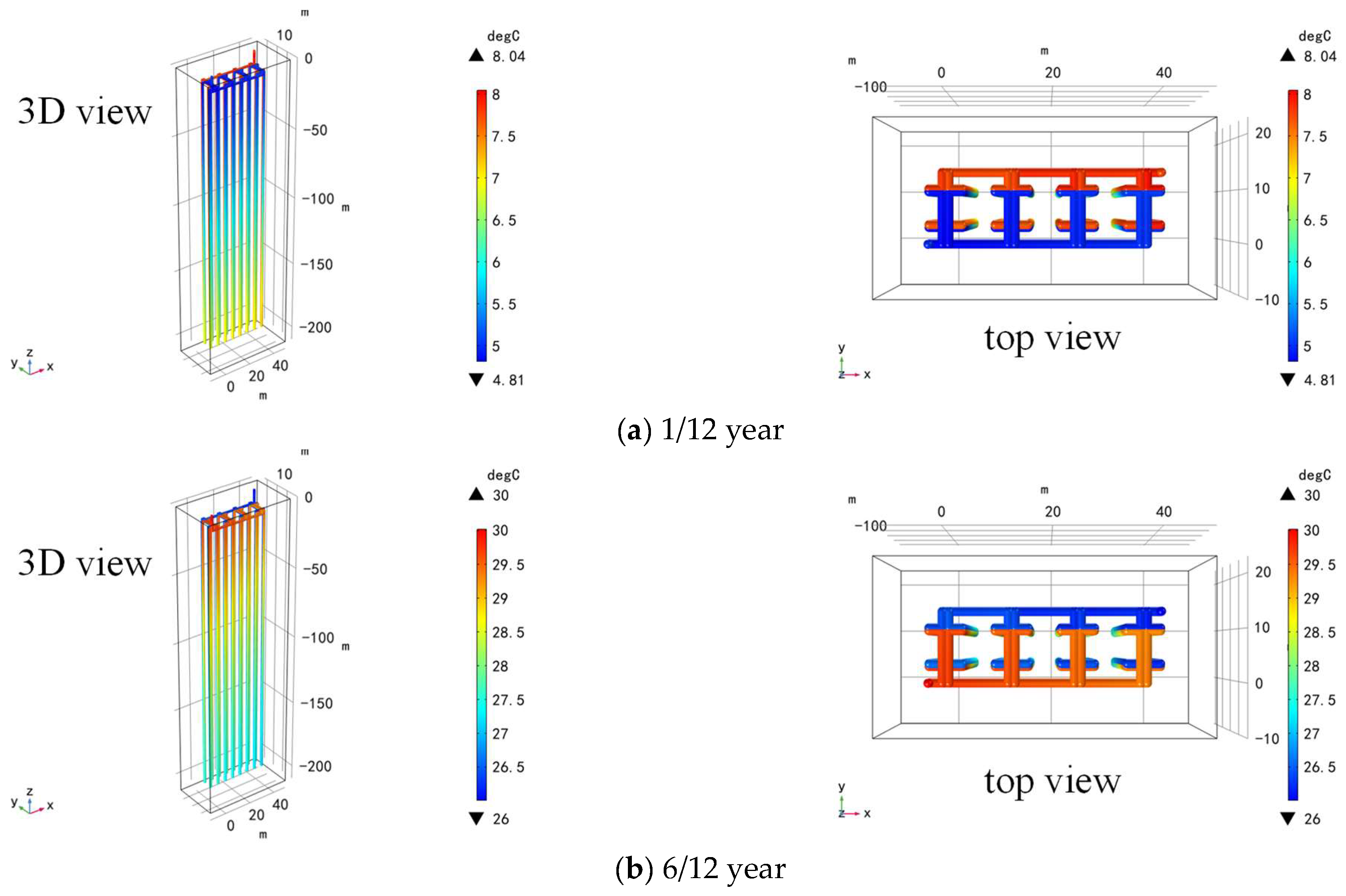
4.2. Temperature Evolution in the Pipeline

The temperature distribution along the pipeline during the operation of SBPS is shown in Figure 9. Figure 9a depicts the heat extraction process in winter by the injection of cold fluid, and it can be drawn that the outlet temperature increases by 3.23 °C compared to the inlet temperature at 1/12 year. Figure 9b depicts the cold extraction process in summer by the injection of hot fluid, and it can be drawn that the outlet temperature decreases by 4 °C compared to the inlet temperature at 6/12 year. Therefore, it is proven that during the alternating process of heat and cold extraction, the low- or high-temperature zone produced in the previous operating cycle has a promoting effect on the outlet temperature increase or decrease in the next operating cycle.

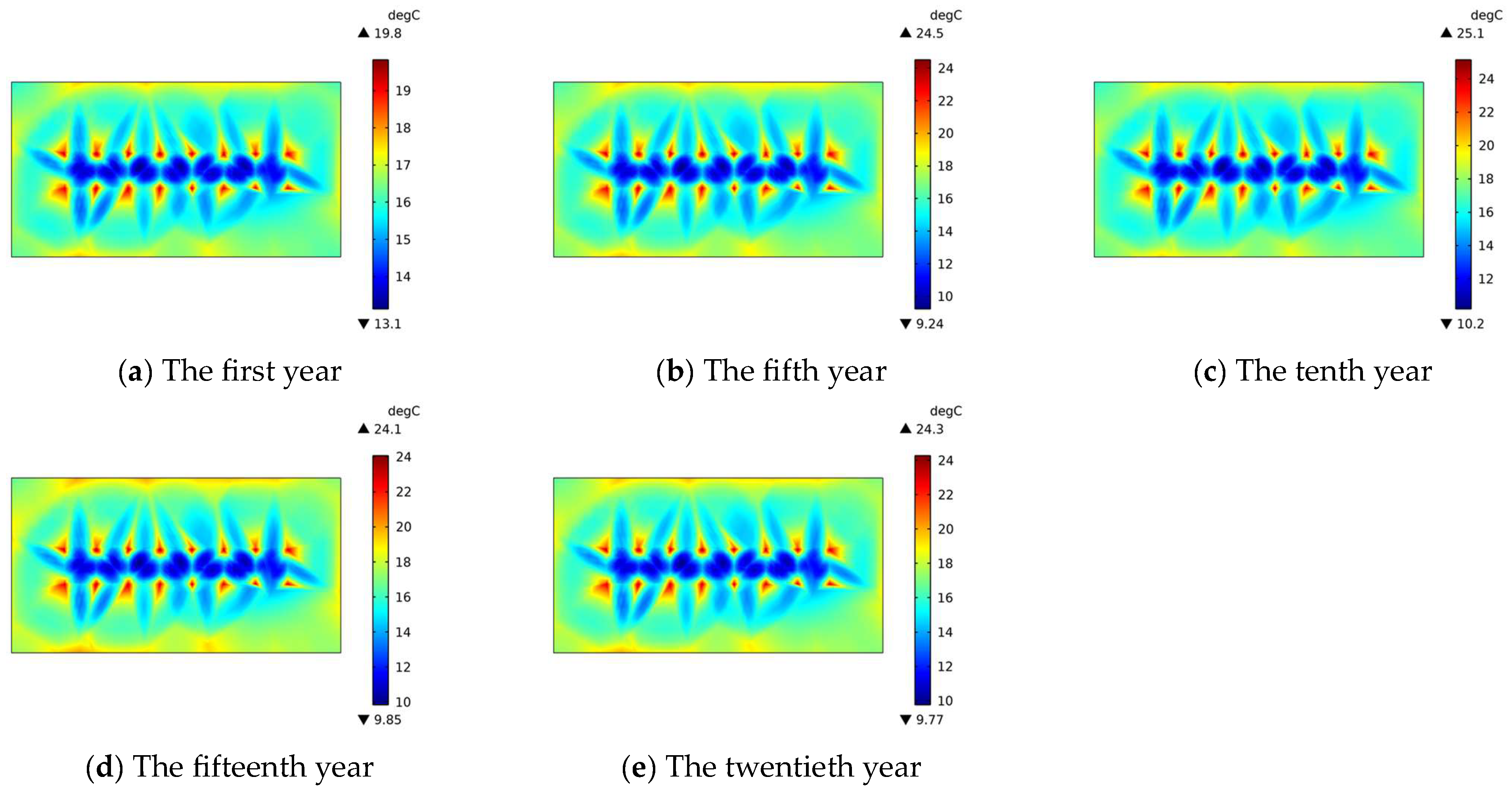
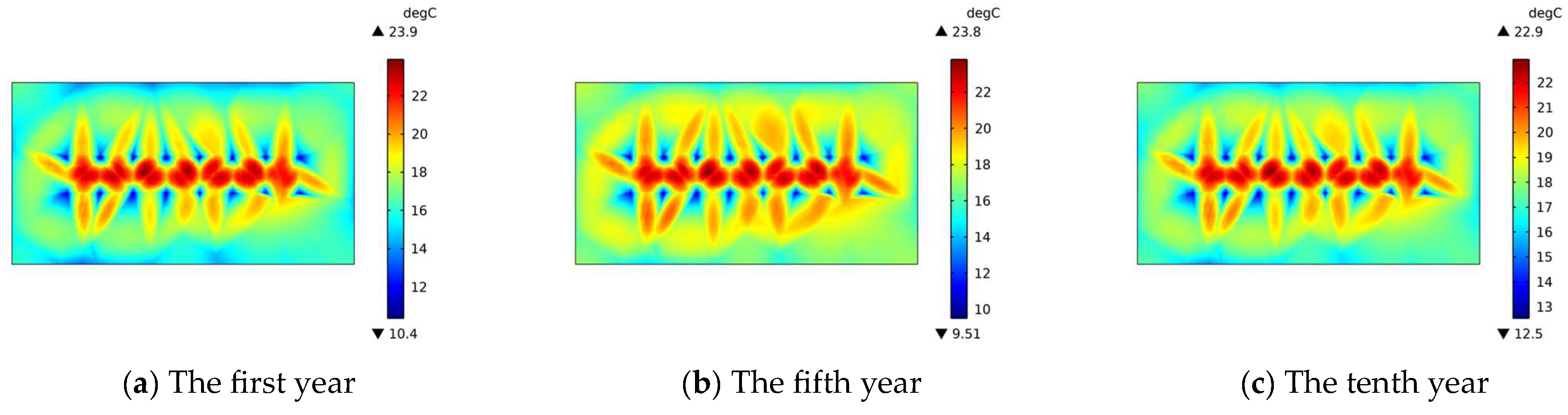
4.3. Temperature Variation with Development Years

It is necessary for the shallow buried pipe system to maintain persistence, and the heat exchange efficiency and heat exchange stability of the shallow buried pipe system are closely related to the evolution of the reservoir temperature field. In this part, the heat transfer simulation of the shallow buried pipe system is carried out for a long time of 20 years. Taking the XY cross section of the underground in −100 m stratum as an indication, the reservoir temperature evolution of the SBPS is studied.

By comparing the temperature distribution of the reservoir temperature field at each operation time in Figure 10 and Figure 11, it can be found that with the alternate operation of the SBPS, the U-shaped tubes are the high-temperature center at the alternation from heat extraction to cold extraction, and the central position between the U-shaped tube heat exchanger groups is the low-temperature center. At the alternation from cold extraction to heat extraction, the U-shaped tube is the low temperature center, the central position of the U-shaped tube group is the high-temperature center, and the relative high-temperature area is in the transition position between the U-shaped tube and the surrounding rock. At the same time, it is found that under the condition that the system is heated for 6 months and cooled for 6 months each year, the temperature distribution rule of the reservoir temperature field corresponding to each running time is similar, and the maximum temperature and the minimum temperature fluctuate in a small range. It shows that with the continuous running, the temperature distribution of the reservoir temperature field of the buried pipe system is relatively regular, and the temperature variation maintains stability, which also proves the stability of the continuous operation of the buried pipe heat exchange system.

5. Sensitivity Analysis

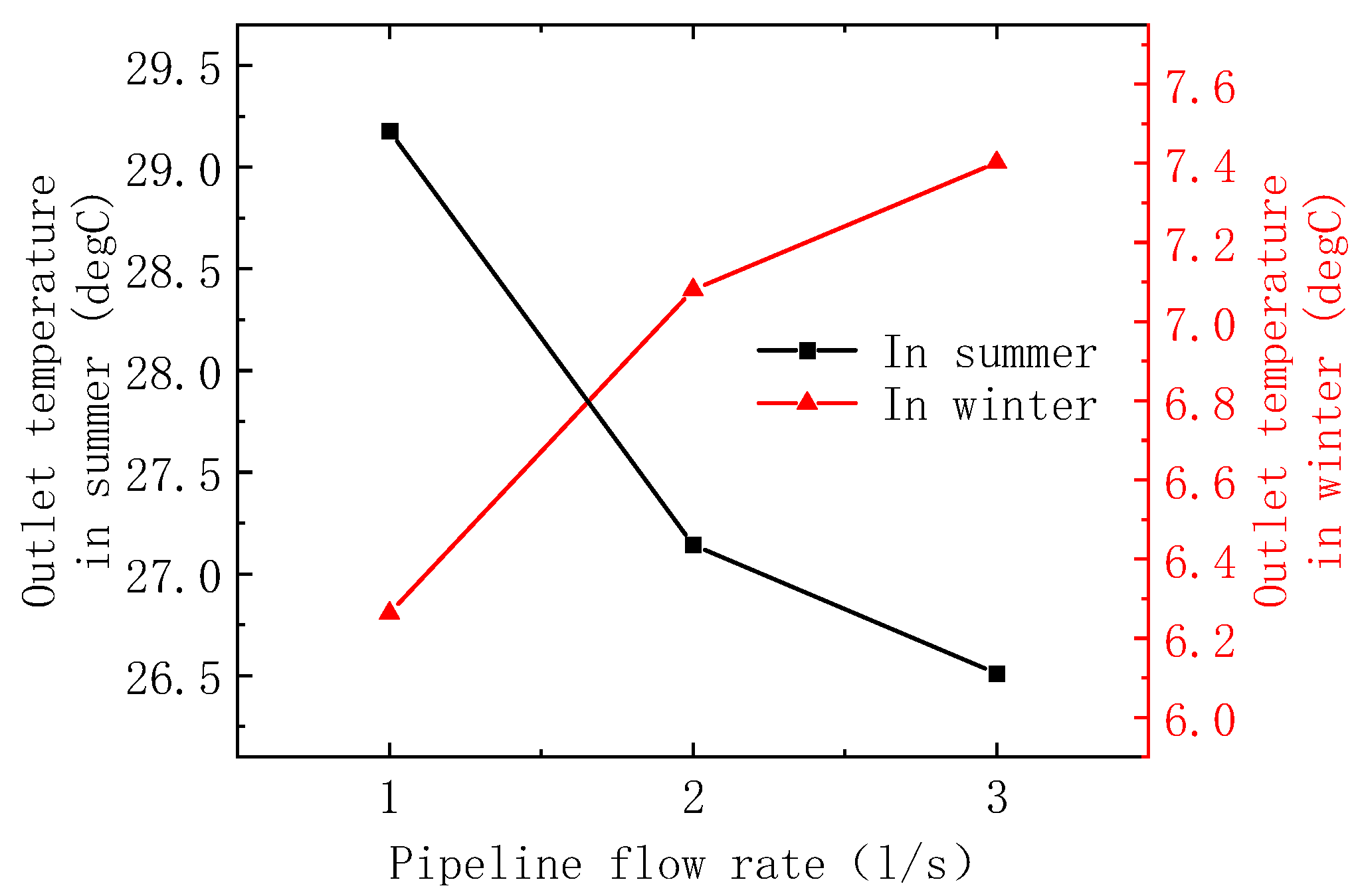
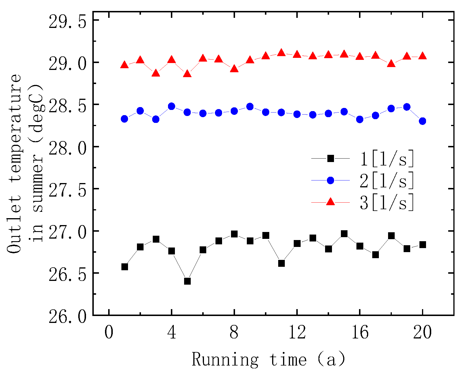
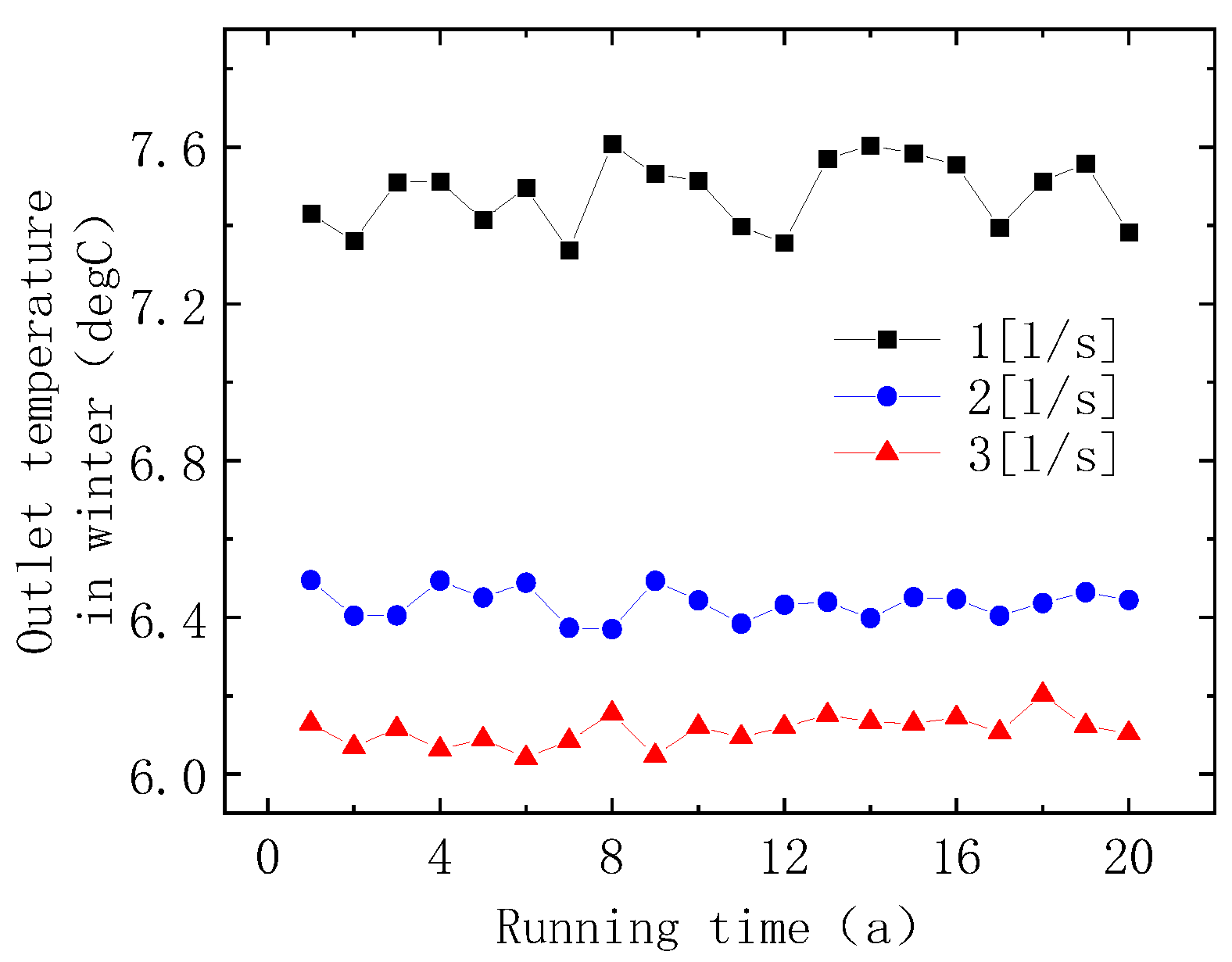
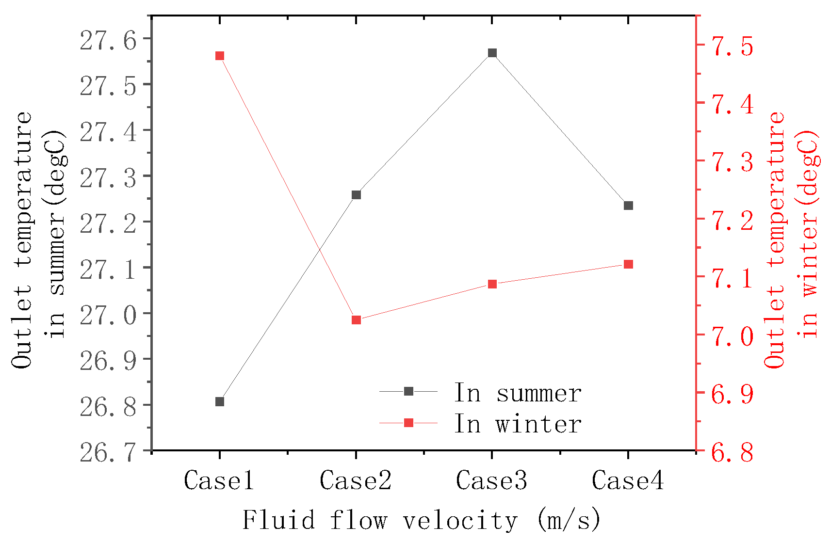
5.1. Effect of Pipeline Flow Rate

The flow velocity of the pipeline is selected as 1[l/s], 2[l/s], and 3[l/s] to simulate the influence of the pipeline flow rate on the heat mining performance of the SBPS.

Figure 12 shows the average values of outlet temperature in summer and winter under different pipeline flow rates of 1 l/s, 2 l/s, and 3 l/s for the heat–cold alternate extraction of 20a. It can be observed that the outlet temperature in summer gradually increases with the increase in flow rate. The average value of outlet temperature in summer increases from 26.8 °C corresponding to the flow rate of 1 l/s to 29.02 °C corresponding to the flow rate of 3 l/s. Summer corresponds to the cooling scenario of the SBPS, and the lower outlet temperature indicates the better heat exchange effect, while the higher outlet temperature indicates the insufficient heat exchange. And with the increase in the flow rate from 1 l/s to 3 l/s, the heat exchange efficiency decreases by 8.27% in summer. For the average value of the outlet temperature in winter, the higher outlet temperature indicates the better heat exchange effect. According to Figure 13, it can be concluded that with the increase in the flow rate, the outlet temperature in winter gradually decreases. The average outlet temperature in winter decreases from 7.48 °C corresponding to the flow rate of 1 l/s to 6.11 °C corresponding to the flow rate of 3 l/s. And the heat exchange efficiency reduces by 18.32%.

Figure 13 and Figure 14 show the outlet temperature variation corresponding to different flow rates in summer and winter. It can be observed that as the flow rate increases, the variation in the maximum and minimum outlet temperature curves shows the tendency of being stable.

Based on the above analysis, it can be concluded that as the flow rate increases, the heat transfer efficiency of the buried pipe system gradually decreases. When the flow rate increases from 1 l/s to 3 l/s, the heat transfer efficiency in winter and summer decreases by 18.32% and 8.27%, respectively. Moreover, as the flow rate increases, the magnitude of the decrease in heat transfer efficiency gradually decreases, indicating that the trend of the decrease in heat transfer efficiency gradually slows down with the increase in flow rate. And with the increase in flow rate, the fluctuation trend of the temperature curve tends to be flattened, which maintains the heat transfer stability of the heat exchange system along the running time.

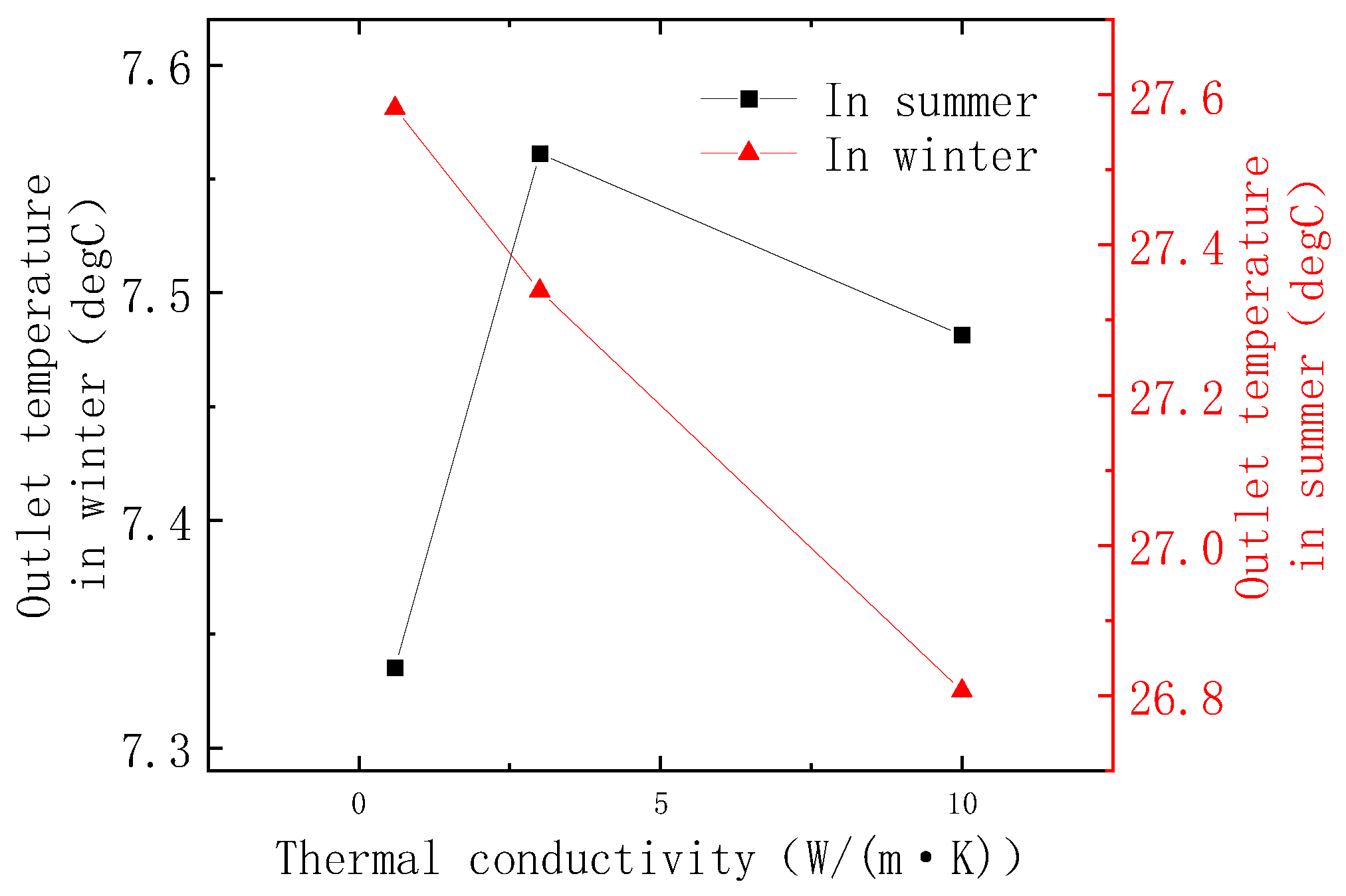
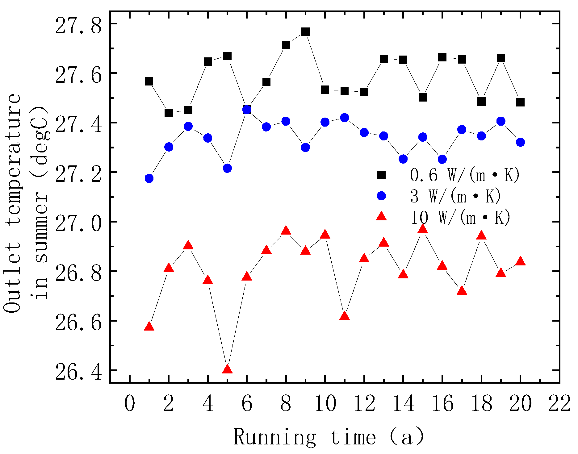
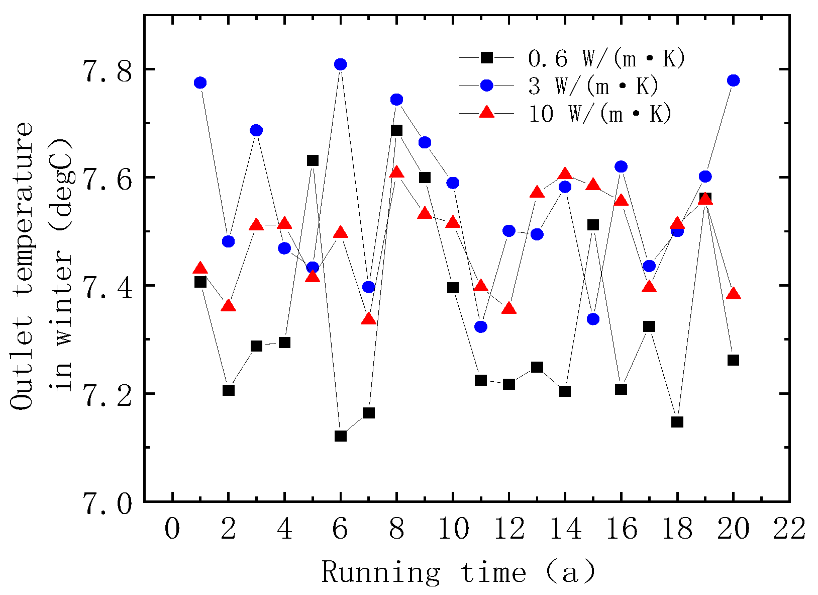
5.2. Effect of Pipeline Wall Thermal Conductivity

We select the buried pipe materials with thermal conductivity coefficients of 0.6 W/(m·K), 3 W/(m·K), and 10 W/(m·K) to analyze the effect of pipeline wall thermal conductivity on the heat mining performance of the SBPS.

Figure 15 shows the average value of the outlet temperature in winter and summer under a different pipeline wall thermal conductivity of 0.6 W/(m·K), 3 W/(m·K), and 10 W/(m·K) for the heat–cold alternate extraction of 20a. It can be observed that with the increase in thermal conductivity, the outlet temperature in summer decreases. The average outlet temperature in summer decreases from 27.58 °C corresponding to the thermal conductivity of 0.6 W/(m·K) to 26.8 °C corresponding to the thermal conductivity of 10 W/(m·K). When the thermal conductivity increases from 0.6 W/(m·K) to 10 W/(m·K), the heat transfer efficiency increases by 2.81%. Winter involves the heat extraction process from the underground formation, as shown in Figure 16; the outlet temperature in winter shows a trend of first increasing and then decreasing with the increase in thermal conductivity. It can be concluded that under heat extraction conditions, setting the thermal conductivity to 3 W/(m·K) can achieve maximum heat exchange efficiency, while, under the cold extraction condition in summer, the higher thermal conductivity will lead to more sufficient heat transfer efficiency. When the thermal conductivity is 10 W/(m·K), the maximum heat transfer efficiency can be achieved.

Figure 16 shows the curve of outlet temperature variation in summer corresponding to different thermal conductivity. The temperature curve with a thermal conductivity of 3 W/(m·K) has significantly less tortuosity than the temperature curve with a thermal conductivity of 0.6 W/(m·K) and 10 W/(m·K), showing better smoothness. Figure 17 shows the curve of outlet temperature variation in winter corresponding to thermal conductivity. It is found that the tortuosity of the thermal conductivity coefficient of 10 W/(m·K) is significantly smaller than the other two curves, showing better smoothness. The operational stability of the SBPS increases with the increase in the thermal conductivity coefficient.

Through analysis, it can be concluded that the heat transfer efficiency of the SBPS increases with the increase in thermal conductivity in summer, while in winter, the heat transfer efficiency first increases and then decreases with the increase in thermal conductivity. Meanwhile, the operational stability increases with the increase in thermal conductivity. Therefore, it is recommended to use pipelines with a thermal conductivity coefficient of 10 W/(m·K) to achieve optimal summer heat transfer efficiency while also considering the heat transfer performance in winter.

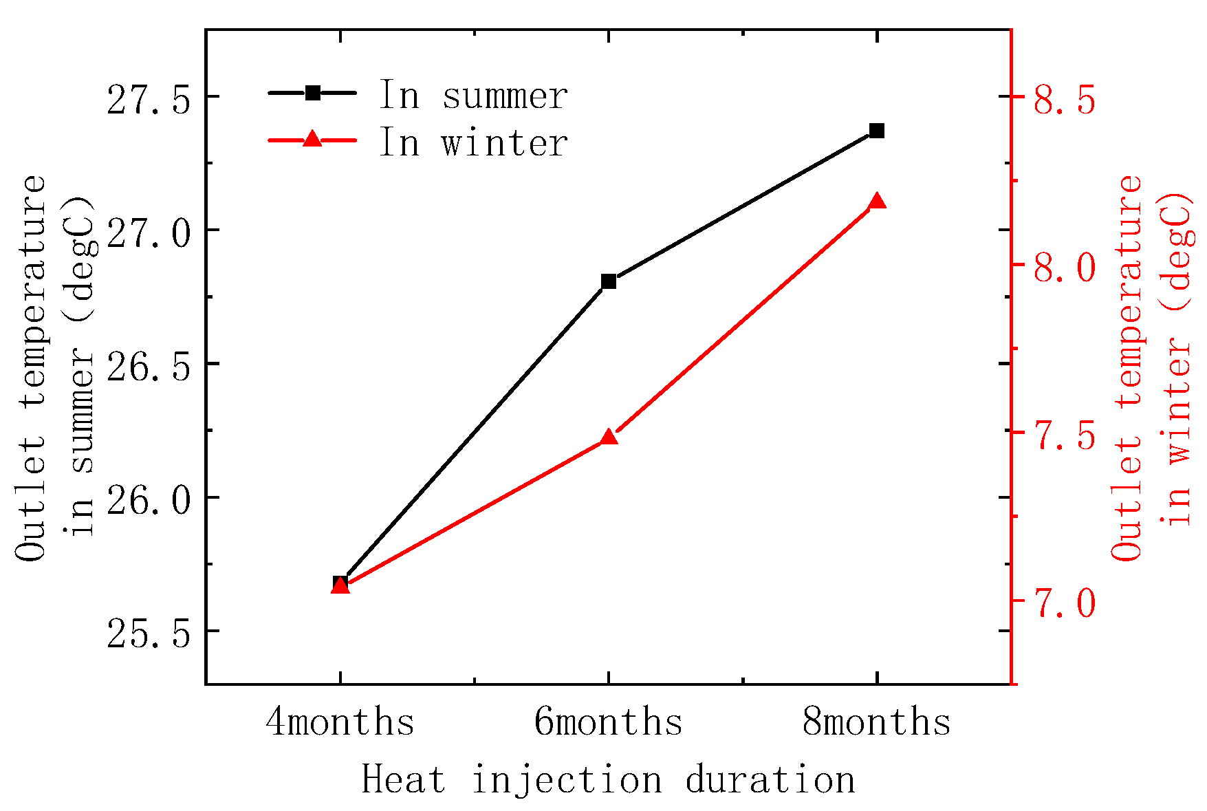
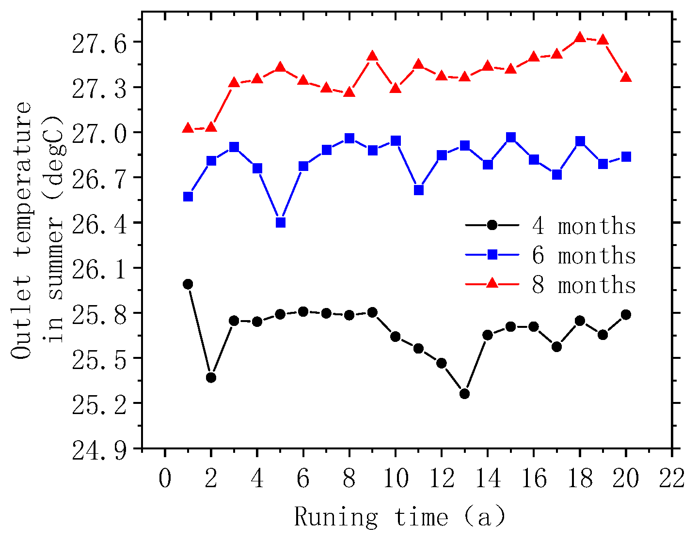
5.3. Effect of Heat Injection Duration

Recently, the use of SBPS for heat storage has also been considered as an effective cross-seasonal energy-storage method [19,36]; thus, we select the heat injection duration of 8 Ms, 6 Ms, and 4 Ms to investigate the operation performance of SBPS, and the heat injection temperature is set to 30 °C.

Figure 18 shows the curve of average outlet temperature in summer and winter under different heat injection durations for the heat–cold alternate extraction of 20a. It can be observed that the average outlet temperature in summer increases with the increase in the heat injection operation time. The average maximum outlet temperature has increased from 25.68 °C corresponding to 4 Ms heat injection to 27.37 °C corresponding to 8 Ms heat injection. Summer corresponds to the cold extraction scenario, and as the heat injection time increases, the heat exchange performance of the SBPS gradually decreases. When the heat injection duration increases from 4 Ms to 6 Ms and 8 Ms, the heat exchange efficiency decreases by 4.39% and 6.59%, respectively, in summer. The outlet temperature in winter increases with the increase in the heat injection time. The heat exchange efficiency for the heat injection duration of 6 Ms and 8 Ms is increased by 6.31% and 16.30% compared to the heat injection of 4 Ms in winter.

Figure 19 shows the curve of outlet temperature variation in summer corresponding to different heat injection operating times, indicating that the heat transfer stability in summer increases with the extension of heat injection time. Figure 20 shows the curve of outlet temperature variation in winter corresponding to the heat injection operating time, which indicates that the heat transfer stability in winter decreases with the extension of heat injection time.

Based on the above analysis, it can be concluded that with the increase in heat injection duration, the variation pattern exhibits the opposite trend in the heat extraction and cold extraction period. The cold extraction efficiency in summer decreases with the increase in heat injection time, while the heat extraction efficiency in winter increases with the increase in heat injection time. When the heat injection time raises from 4 Ms to 8 Ms, the cold extraction efficiency in summer decreases by 6.59%, and the heat extraction efficiency in winter increases by 16.30%. In addition, as the heat injection time increases, the trend of the outlet temperature variation in summer tends to be gentle, while the trend of the outlet temperature variation in winter tends to become steeper. Therefore, the consistent heat and cold injection time throughout the year is beneficial for the long-term stable operation of the shallow buried pipe system.

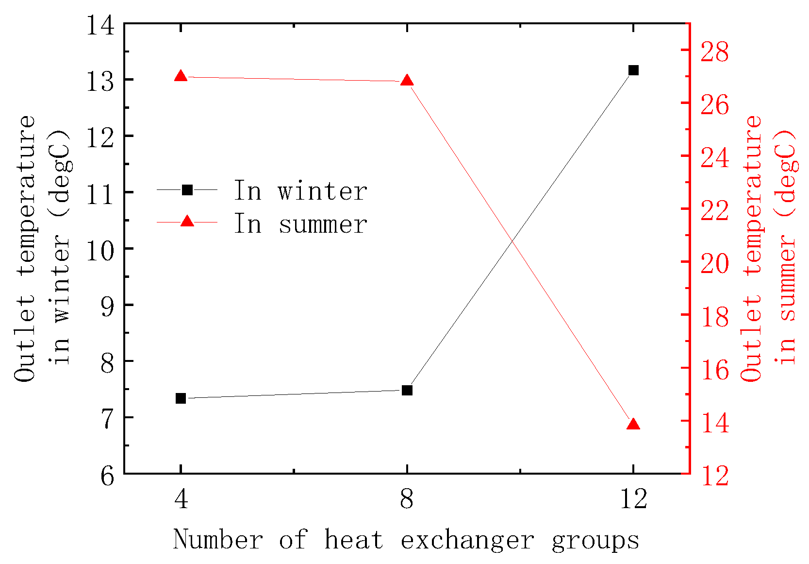
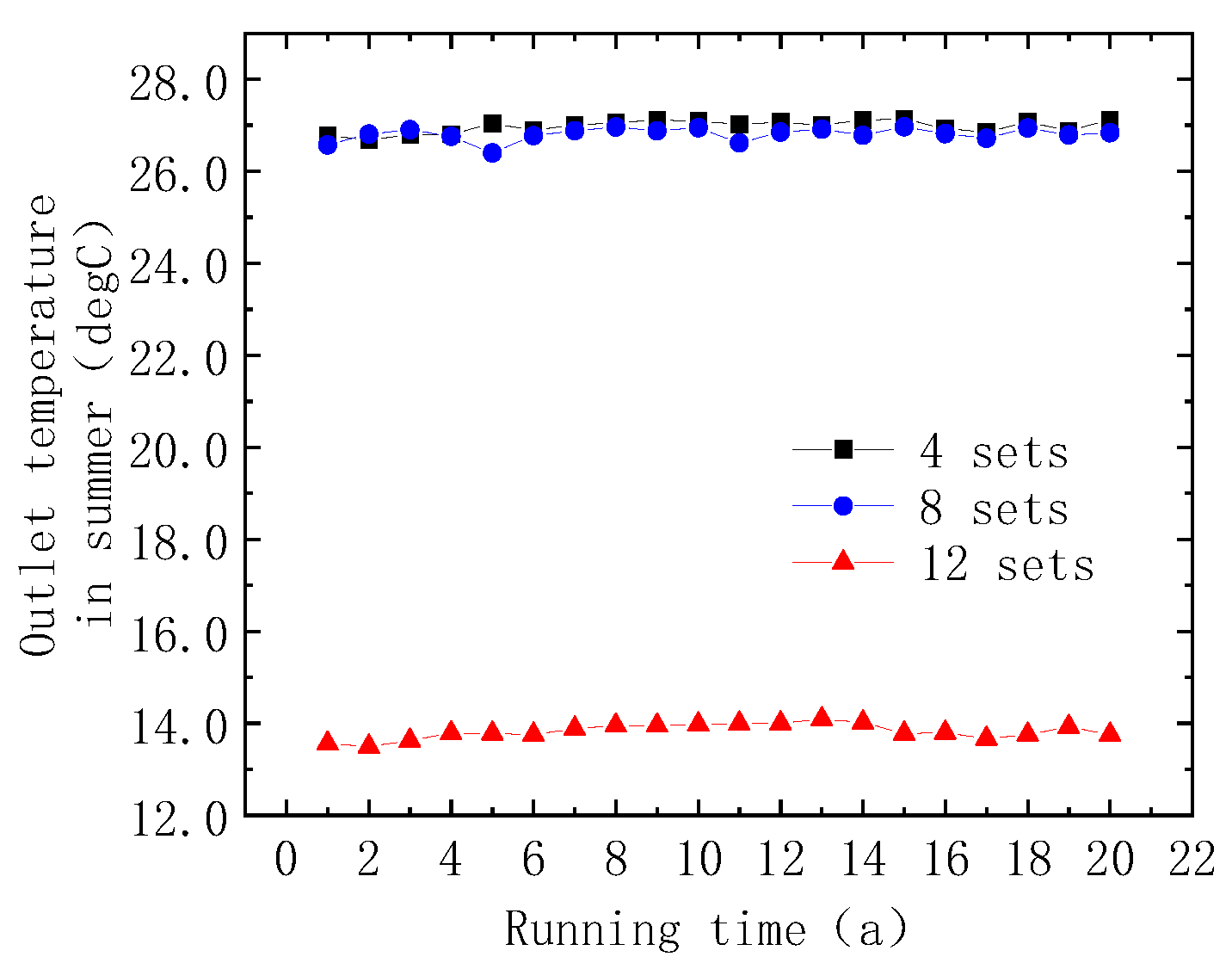
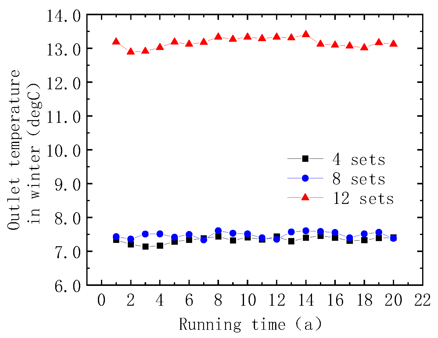
5.4. Effect of the Number of Heat Exchanger Groups

To clarify the impact of the number of buried pipe heat exchanger groups on heat mining performance, we select 4, 8, and 12 sets of U-shaped tube heat exchanger groups for heat mining simulation.

Figure 21 shows the average outlet temperature in summer and winter under different numbers of U-shaped tube heat exchanger groups for the heat–cold alternate extraction of 20a. It can be observed that the average values of the outlet temperature in summer decrease with the increase in the number of U-shaped tube heat exchanger groups. The average outlet temperature decreases from 26.97 °C corresponding to 4 sets of U-shaped tube heat exchangers to 13.83 °C corresponding to 12 sets of U-shaped tube heat exchangers. In addition, the decrease in the average outlet temperature in summer is significantly greater when the heat exchanger groups are added from 8 sets to 12 sets relative to that from 4 sets to 8 sets. Summer corresponds to the cold extraction scenario, and as the number of U-shaped tube heat exchanger groups increases from 4 to 8 and 12 sets, the heat exchange efficiency increases by 0.62% and 48.73%, respectively. For the heat extraction process in winter, the heat exchange efficiency of 8 sets of heat exchangers and 12 sets of heat exchangers increased by 1.96% and 79.46% compared to 4 sets of U-shaped tube heat exchangers, respectively.

Figure 22 shows the curve of outlet temperature variation in summer corresponding to different U-shaped tube heat exchanger groups. The heat exchange stability of the heat exchange system in summer increases with the increase in the number of heat exchanger groups. Figure 23 shows the curve of outlet temperature variation in winter corresponding to different U-shaped tube heat exchanger groups. It can be drawn that the heat transfer stability of the heat exchange system in winter decreases with the raise of the number of heat exchanger groups.

Based on the above analysis, it can be concluded that as the number of U-shaped tube heat exchanger groups increases, the heat transfer efficiency of the SBPS improves significantly. When the number of heat exchanger groups increases from 4 sets to 12 sets, the heat transfer efficiency in winter and summer increases by 48.73% and 79.46%, respectively. In addition, with the increase in the number of heat exchanger groups, the variation pattern of the heat transfer stability in cooling and heating conditions is different. The stability under cooling conditions in summer increases with the increase in heat exchanger groups, while the stability under heating conditions in winter decreases with the increase in heat exchanger groups.

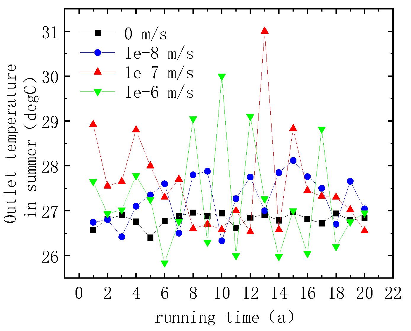
5.5. Effect of Groundwater Flow

To clarify the impact of fluid flow velocity on heat mining performance, we select 0, 1 × 10⁻⁸, 1 × 10⁻⁷, and 1 × 10⁻⁶ m/s as the fluid flow velocity of groundwater in the reservoir for heat mining simulation [45].

Figure 24 shows the average outlet temperature in summer and winter under different fluid flow velocity for the heat–cold alternate extraction of 20a. It can be observed that the outlet temperature presents the trend of first an increase and then a decrease with the increase in groundwater flow velocity in summer. The outlet temperature reaches the maximum value of 27.569 °C at the flow velocity of 1 × 10⁻⁷ m/s, and then decreases with the increase in the flow velocity. And the outlet temperature presents the trend of first a decrease and then an increase with the increase in fluid flow velocity in winter. The maximum value of the outlet temperature is 7.481 °C when the flow velocity is 0 m/s, and the minimum value is 7.025 °C when the flow velocity is 1 × 10⁻⁸ m/s.

Figure 25 and Figure 26 respectively show the curve of outlet temperature variation in summer and winter corresponding to different groundwater flow velocity. As can be seen, the heat exchange stability of the heat exchange system decreases with the increase in the groundwater flow velocity. Thus, the stability of SBPS decreases with the increase in the groundwater flow velocity in winter and summer.

In Part 4.1, it has been proven that the heat exchange in the previous operation cycle will promote the extraction of heat or cold in the next operation cycle during the development of the SBPS, which is benefited by the heat or cold accumulation around the buried pipe during the previous operation cycle. When there is no groundwater flow in the shallow reservoir, the energy accumulation will play the dominant role, while when the groundwater begins to flow, the energy accumulation effect will be weakened. However, with the increase in the groundwater flow velocity, the recovery ability of the underground temperature field will be enhanced, then the heat transfer efficiency of SBPS will be improved. When the groundwater flow velocity exceeds 1 × 10⁻⁷ m/s, the recovery of the temperature field driven by groundwater flow will play the dominant role. Therefore, with the increase in groundwater flow velocity, the heat transfer efficiency shows the trend of first decreasing and then increasing.

6. Conclusions

(1)

During the alternating process of heat and cold extraction, the low- or high-temperature zone produced in the previous operating cycle has the promoting effect on the rise or decrease in outlet temperature in the next operating cycle;

(2)

When the heat extraction (with the injection temperature of 5 °C) and cold extraction (with the injection temperature of 30 °C) duration are consistent each year, it is beneficial to maintain the long-term stable operation for the shallow buried pipe system;

(3)

As the pipeline flow rate increases, the heat transfer efficiency of the buried pipe system gradually decreases. When the flow rate increases from 1 l/s to 3 l/s, the heat transfer efficiency in winter and summer decreases by 18.32% and 8.27%, respectively;

(4)

The heat transfer efficiency of the SBPS increases with the increase in thermal conductivity in summer, while in winter, the heat transfer efficiency first increases and then decreases with the raise of thermal conductivity. In addition, the operation stability increases with the increase in thermal conductivity;

(5)

The cold extraction efficiency in summer decreases with the increase in the heat injection time, while the heat extraction efficiency in winter increases with the increase in the heat injection time. When the heat injection time raises from 4 Ms to 8 Ms, the cold extraction efficiency in summer decreases by 6.59%, and the heat extraction efficiency in winter increases by 16.30%. Therefore, the consistent heat and cold injection time throughout the year is beneficial for the long-term stable operation of the shallow buried pipe system;

(6)

As the number of U-shaped tube heat exchanger groups increases, the heat transfer efficiency of the SBPS improves significantly. When the number of heat exchanger groups increases from 4 to 12, the heat transfer efficiency in winter and summer increases by 48.73% and 79.46%, respectively. In addition, as the number of heat exchanger groups increases, the variation pattern of heat transfer stability in cooling and heating condition is different. The stability under cooling conditions in summer increases with the increase in heat exchanger groups, while the stability under heating conditions in winter decreases with the increase in heat exchanger groups;

(7)

When there is no groundwater flow in the shallow reservoir, the energy accumulation will play the dominant role, while when the groundwater begins to flow, the energy accumulation effect will be weakened. However, with the increase in the groundwater flow velocity, the recovery ability of the underground temperature field will be enhanced, then the heat transfer efficiency of the SBPS will be improved.

In this research, the heat transfer mechanism of the heat–cold alternate extraction in a shallow buried pipe system under multiple heat exchanger groups is revealed based on the flow and heat transfer model in the pipeline and reservoir. In addition, the influence of pipeline flow rates, pipeline wall thermal conductivity, heat injection durations, the numbers of heat exchanger groups, and the flows of underground fluid on heat transfer efficiency is also investigated. In future work, the experimental research based on the self-developed equipment will be conducted.

References

1. Zhang, X.P.; Li, G.; Han, Z.W.; Yang, Z.W.; Bi, W.; Li, X.; Yang, L. Study on the influence of buried pipe fault on the operation of ground source heat pump system. Renew. Energy 2023, 210, 12–25. [Google Scholar] [CrossRef]
2. Gigot, V.; Francois, B.; Huysmans, M.; Gerard, P. Monitoring of the thermal plume around a thermally activated borehole heat exchanger and characterization of the ground hydro-geothermal parameters. Renew. Energy 2023, 218, 119250. [Google Scholar] [CrossRef]
3. Hou, G.; Taherian, H.; Li, L. A predictive TRNSYS model for long-term operation of a hybrid ground source heat pump system with innovative horizontal buried pipe type. Renew. Energy 2020, 151, 1046–1054. [Google Scholar] [CrossRef]
4. De León-Ruiz, J.E.; Beltrán-Chacón, R.; Carvajal-Mariscal, I.; Zacarías, A.; Rodríguez-Maese, R. A data-driven approach to low-enthalpy shallow geothermal energy extraction: A case study on indoor heating for precision agriculture applications. Case Stud. Therm. Eng. 2022, 40, 102578. [Google Scholar] [CrossRef]
5. Dalla Santa, G.; Galgaro, A.; Sassi, R.; Cultrera, M.; Scotton, P.; Mueller, J.; Bertermann, D.; Mendrinos, D.; Pasquali, R.; Perego, R.; et al. An updated ground thermal properties database for GSHP applications. Geothermics 2020, 85, 101758. [Google Scholar] [CrossRef]
6. Sun, Y.X.; Zhang, X.; Li, X.H.; Cheng, R. Study on the intrinsic mechanisms underlying enhanced geothermal system (EGS) heat transfer performance differences in multi-wells. Energy Convers. Manag 2023, 292, 117361. [Google Scholar] [CrossRef]
7. Perego, R.; Dalla Santa, G.; Galgaro, A.; Pera, S. Intensive thermal exploitation from closed and open shallow geothermalsystems at urban scale: Unmanaged conflicts and potential synergies. Geothermics 2022, 103, 102417. [Google Scholar] [CrossRef]
8. Li, W.J.; Zhang, W.K.; Li, Z.X.; Yao, H.; Cui, P.; Zhang, F. Investigation of the Heat Transfer Performance of Multi-Borehole Double-Pipe Heat Exchangers in Medium-Shallow Strata. Energies 2022, 15, 134798. [Google Scholar] [CrossRef]
9. Galgaro, A.; Dalla Santa, G.; Zarrella, A. First Italian TRT database and significance of the geological settingevaluation in borehole heat exchanger sizing. Geothermics 2021, 94, 102098. [Google Scholar] [CrossRef]
10. Kerme, E.D.; Fung, A.S. Heat transfer analysis of single and double U-tube borehole heat exchanger with two independent circuits. J. Energy Storage 2021, 43, 103141. [Google Scholar] [CrossRef]
11. Jahanbin, A. Thermal performance of the vertical ground heat exchanger with a novel elliptical single U-tube. Geothermics 2020, 86, 101804. [Google Scholar] [CrossRef]
12. Chen, Z.; Lian, X.W.; Tan, J.J.; Xiao, H.; Ma, Q.; Zhuang, Y. Study on heat-exchange efficiency and energy efficiency ratio of a deeply buried pipe energy pile group considering seepage and circulating-medium flow rate. Renew. Energy 2023, 216, 119020. [Google Scholar] [CrossRef]
13. Cai, Y. Research on the Influencing Factors of Heat Exchange Capacity of Vertical Buried Tube Heat Exchanger. Master’s Thesis, China University of Geosciences (Beijing), Beijing, China, 2020. (In Chinese). [Google Scholar]
14. Li, L.; Fu, Z.; Li, B.; Zhu, Q. Comparison of Thermal Performance for Two Types of ETFP System under Various Operation Schemes. Comput. Model. Eng. 2020, 124, 23–44. [Google Scholar] [CrossRef]
15. Chen, K.; Zhang, J.; Li, J.; Shao, J.; Zhang, Q. Numerical study on the heat performance of enhanced coaxial borehole heat exchanger and double U borehole heat exchanger. Appl. Therm. Eng. 2022, 203, 117916. [Google Scholar] [CrossRef]
16. Zhou, H.; Liu, J.; Li, T. Applicability of the pipe structure and flow velocity of vertical ground heat exchanger for ground source heat pump. Energy Build. 2016, 117, 109–119. [Google Scholar] [CrossRef]
17. Harris, B.E.; Lightstone, M.F.; Reitsma, S.; Cotton, J.S. Analysis of the transient performance of coaxial and u-tube borehole heat exchangers. Geothermics 2022, 101, 102319. [Google Scholar] [CrossRef]
18. Wang, Y.; Duan, M.; Zhang, Y. Experimental and numerical investigation of vertical pipe–soil interaction considering pipe velocity. Ships Offshore Struct. 2017, 12, 1112178. [Google Scholar] [CrossRef]
19. Jahanbin, A.; Semprini, G.; Pulvirenti, B. Performance evaluation of U-tube borehole heat exchangers employing nanofluids as the heat carrier fluid. Appl. Therm. Eng. 2022, 212, 118625. [Google Scholar] [CrossRef]
20. Li, J.; Zheng, J.; Lei, X.D.; Jia, Z.; Liu, A.; Xu, Z. Influence of geologic conditions and buried pipe form on the heat transfer performance of buried pipe heat exchangers. Earth J. 2022, 44, 211–229. (In Chinese) [Google Scholar]
21. Ye, W.J.; Dong, X.H.; Yang, G.S.; Chen, Q.; Peng, R.; Liu, K. Effect of moisture content and dry density on thermal parameters of loes. Rock Soil Mech. 2017, 38, 656–662. (In Chinese) [Google Scholar]
22. Florides, G.; Christodoulides, P.; Pouloupatis, P. Single and double U-tube ground heat exchangers in multiple-layer substrates. Appl. Energy 2013, 102, 364–373. [Google Scholar] [CrossRef]
23. Du, J.; Luo, Z.; Ge, W. Study on the simulation and optimization of the heat transfer scheme in a buried-pipe ground-source heat pump. Arab. J. Geosci. 2020, 13, 437–443. [Google Scholar] [CrossRef]
24. Yue, G.F. Numerical simulation study on soil temperature field influenced by GSHP: A case study in Beijing. China Sci. 2017, 12, 1049–1053. (In Chinese) [Google Scholar]
25. DiCarlo, A.A. Novel seasonal enhancement of shallow ground source heat pumps. Appl. Therm. Eng. 2021, 186, 116510. [Google Scholar] [CrossRef]
26. Wang, L.; Ren, Y.L.; Deng, F.Q.; Zhang, Y.; Qiu, Y. Study on Calculation Method of Heat Exchange Capacity and Thermal Properties of Buried Pipes in the Fractured Rock Mass-Taking a Project in Carbonate Rock Area as an Example. Energies 2023, 16, 020774. [Google Scholar] [CrossRef]
27. Fei, Y.C.; Zhou, Y.S.; Zhao, L.Y.; Zhang, Y.C. Effect of compound additives on performance of buried pipe grouting material. J. Donghua Univ. (Nat. Sci.) 2018, 44, 966–972. (In Chinese) [Google Scholar]
28. Xu, Y.J.; Huang, X.W.; Fang, Y.; Shu, S.; Zhu, H. Heat transfer characteristics and heat conductivity prediction model of waste steel slag–clay backfill material. Therm. Sci. Eng. Prog. 2023, 46, 102203. [Google Scholar] [CrossRef]
29. Song, X.; Jiang, M.; Qin, P. Numerical investigation of the backfilling material thermal conductivity impact on the heat transfer performance of the buried pipe heat exchanger. IOP Conf. Ser. Earth Environ. Sci. 2019, 267, 042010. [Google Scholar] [CrossRef]
30. Mascarin, L.; Garbin, E.; Di Sipio, E.; Dalla Santa, G.; Bertermann, D.; Artioli, G.; Bernardi, A.; Galgaro, A. Selection of backfill grout for shallow geothermal systems: Materials investigation and thermo-physical analysis. Constr. Build. Mater. 2022, 318, 125832. [Google Scholar] [CrossRef]
31. Peng, J.; Li, Q.; Huang, C. A New Environmentally Friendly Utilization of Energy Piles into Geotechnical Engineering in Northern China. Adv. Civ. Eng. 2021, 2021, 4689062. [Google Scholar] [CrossRef]
32. Liu, C.; Yu, G.; Jia, S. A Quasi-Three Dimensional Transient Model for Thermal Calculation of Buried Pipe Heat Exchanger Systems. In Proceedings of the International Conference on Computational & Experimental Engineering and Sciences, Tokyo, Japan, 25–28 March 2019; Volume 22, p. 156. [Google Scholar]
33. Wang, F.; You, T. Synergetic performance improvement of a novel building integrated photovoltaic/thermal-energy pile system for co-utilization of solar and shallow-geothermal energy. Energy Convers. Manag. 2023, 288, 1117116. [Google Scholar] [CrossRef]
34. Chen, G.; Fan, H.; Wang, E.; Shen, H.; Zhang, X.; Wang, Z. Research on the Performance of Solar Energy Buried Pipe Heat Exchanger for Heating Landfill Technology. Sol. Energy 2023, 5, 69–77. [Google Scholar]
35. Wei, Y.Q.; Kong, G.Q.; Zhang, J.B.; Yang, Q. Heat transfer efficiency of energy tunnel influenced by inlet temperature, flow rate and pipe spacing. IOP Conf. Ser. Earth Environ. Sci. 2021, 861, 072125. [Google Scholar] [CrossRef]
36. Naranjo-Mendoza, C.; Oyinlola, M.A.; Wright, A.J.; Greenough, R.M. Experimental study of a domestic solar-assisted ground source heat pump with seasonal underground thermal energy storage through shallow boreholes. Appl. Therm. Eng. 2019, 162, 114218. [Google Scholar] [CrossRef]
37. Shi, Y.; Cui, Q.L.; Yang, Z.J.; Song, X.; Liu, Q.; Lin, T. Optimizing the thermal energy storage performance of shallow aquifers based on gray correlation analysis and multi-objective optimization. Nat. Gas Ind. B 2023, 10, 476–489. [Google Scholar] [CrossRef]
38. Harjunowibowo, D.; Omer, S.A.; Riffat, S.B. Experimental investigation of a ground-source heat pump system for greenhouse heating–cooling. Int. J. Low-Carbon Technol. 2021, 16, 1529–1541. [Google Scholar] [CrossRef]
39. Nagare, R.M.; Mohammed, A.A.; Park, Y.J.; Schincariol, R.A. Modeling shallow ground temperatures around hot buried pipelines in cold regions. Cold Reg. Sci. Technol. 2021, 187, 103295. [Google Scholar] [CrossRef]
40. Hoseinzadeh, S.; Heyns, P. Thermo-structural fatigue and lifetime analysis of a heat exchanger as a feedwater heater in power plant. Eng. Fail. Anal. 2020, 113, 104548. [Google Scholar] [CrossRef]
41. Alizadeh, A.; Ghadamian, H.; Aminy, M.; Hoseinzadeh, S.; Sahebi, H.K.; Sohani, A. An experimental investigation on using heat pipe heat exchanger to improve energy performance in gas city gate station. Energy 2022, 252, 123959. [Google Scholar] [CrossRef]
42. COMSOL. Multiphysics User’s Guide, Version 6.1; COMSOL Inc.: Burlington, MA, USA, 2023; Available online: https://www.comsol.com (accessed on 1 November 2022).
43. Zhang, W.; Wang, C.G.; Guo, T.K.; He, J.; Zhang, L.; Chen, S.; Qu, Z. Study on the cracking mechanism of hydraulic and supercritical CO2 fracturing in hot dry rock under thermal stress. Energy 2021, 221, 119886. [Google Scholar] [CrossRef]
44. Zhang, W.; Wang, Z.L.; Guo, T.K.; Wang, C.; Li, F.; Qu, Z. The enhanced geothermal system heat mining prediction based on fracture propagation simulation of thermo-hydro-mechanical-damage coupling: Insight from the integrated research of heat mining and supercritical CO2 fracturing. Appl. Therm. Eng. 2022, 215, 118919. [Google Scholar] [CrossRef]
45. Dalla Santa, G.; Schincariol, A.R. Effect of thermal-hydrogeological and borehole heat exchanger properties on performance and impact of vertical closed-loop geothermal heat pump systems. Hydrogeol. J. 2014, 22, 189–203. [Google Scholar]
Figure 1. The operation process of U-shaped buried pipes heat exchanger.
Energies 16 08067 g001
Figure 2. Schematic diagram of the simulation model.
Energies 16 08067 g002aEnergies 16 08067 g002b
Figure 3. The inlet temperature.
Energies 16 08067 g003
Figure 4. The surface temperature.
Energies 16 08067 g004
Figure 5. The initial temperature distribution: (a) the 3D view of temperature distribution; (b) the XY cross-section of the 2D temperature distribution buried in −100 m depth; (c) the YZ cross-section of the 2D temperature distribution.
Energies 16 08067 g005
Figure 6. The temperature distribution in heat extraction process (1/12 year represents the first month of the year; 2/12 year represents the second month of the year; 3/12 year represents the third month of the year).
Energies 16 08067 g006
Figure 7. The temperature distribution in the cold extraction process.
Energies 16 08067 g007
Figure 8. The temperature distribution in the alternation process: (a) heat extraction to cold extraction (5/12 year), (b) cold extraction to heat extraction (10/12 year).
Energies 16 08067 g008
Figure 9. The temperature distribution in the pipeline.
Energies 16 08067 g009
Figure 10. Temperature field distribution at the alternation from heat extraction to cold extraction at the buried depth of −100 m.
Energies 16 08067 g010
Figure 11. Temperature field distribution at the alternation from cold extraction to heat extraction at the buried depth of −100 m.
Energies 16 08067 g011aEnergies 16 08067 g011b
Figure 12. The average value of the maximum (in summer) and the minimum (in winter) outlet temperature with different flow rates.
Energies 16 08067 g012
Figure 13. Maximum outlet temperature (in summer) under different flow rates.
Energies 16 08067 g013
Figure 14. Minimum outlet temperature (in winter) under different flow rates.
Energies 16 08067 g014
Figure 15. The average value of outlet temperature in summer and winter with different thermal conductivity of pipeline wall.
Energies 16 08067 g015
Figure 16. Outlet temperature in summer under different thermal conductivity.
Energies 16 08067 g016
Figure 17. Outlet temperature in winter under different thermal conductivity.
Energies 16 08067 g017
Figure 18. The average value of outlet temperature in summer and winter with different heat injection durations.
Energies 16 08067 g018
Figure 19. Outlet temperature in summer under different heat injection durations.
Energies 16 08067 g019
Figure 20. Outlet temperature in winter under different heat injection durations.
Energies 16 08067 g020
Figure 21. The average value of outlet temperature in summer and winter with a different number of heat exchanger groups.
Energies 16 08067 g021
Figure 22. Outlet temperature in summer under a different number of heat exchanger groups.
Energies 16 08067 g022
Figure 23. Outlet temperature in winter under a different number of heat exchanger groups.
Energies 16 08067 g023
Figure 24. The average value of outlet temperature in summer and winter with different groundwater flow velocity (Case 1 represents the fluid flow velocity of 0 m/s; Case 2 represents the fluid flow velocity of 1 × 10⁻⁸ m/s; Case 3 represents the fluid flow velocity of 1 × 10⁻⁷ m/s; Case 4 represents the fluid flow velocity of 1 × 10⁻⁶ m/s).
Energies 16 08067 g024
Figure 25. Outlet temperature in summer under different groundwater flow velocity.
Energies 16 08067 g025
Figure 26. Outlet temperature in winter under different groundwater flow velocity.
Energies 16 08067 g026