Article

Grid Distribution Fault Occurrence and Remedial Measures Prediction/Forecasting through Different Deep Learning Neural Networks by Using Real Time Data from Tabuk City Power Grid

by
Fahad M. Almasoudi
Department of Electrical Engineering, Faculty of Engineering, University of Tabuk, Tabuk 47913, Saudi Arabia
Energies 2023, 16(3), 1026; https://doi.org/10.3390/en16031026
Submission received: 30 December 2022 / Revised: 11 January 2023 / Accepted: 13 January 2023 / Published: 17 January 2023
(This article belongs to the Section F5: Artificial Intelligence and Smart Energy)

Abstract

:
Modern societies need a constant and stable electrical supply. After relying primarily on formal mathematical modeling from operations research, control theory, and numerical analysis, power systems analysis has changed its attention toward AI prediction/forecasting tools. AI techniques have helped fix power system issues in generation, transmission, distribution, scheduling and forecasting, etc. These strategies may assist today’s large power systems which have added more interconnections to meet growing load demands. They make it simple for them to do difficult duties. Identification of problems and problem management have always necessitated the use of labor. These operations are made more sophisticated and data-intensive due to the variety and growth of the networks involved. In light of all of this, the automation of network administration is absolutely necessary. AI has the potential to improve the problem-solving and deductive reasoning approaches used in fault management. This study implements a variety of artificial intelligence and deep learning approaches in order to foresee and predict the corrective measures that will be conducted in response to faults that occur inside the power distribution network of the Grid station in Tabuk city with regard to users. The Tabuk grid station is the source of the data that was gathered for this purpose; it includes a list of defects categorization, actions and remedies that were implemented to overcome these faults, as well as the number of regular and VIP users from 2017 to 2022. Deep learning, the most advanced method of learning used by artificial intelligence, is continuing to make significant strides in a variety of domain areas, including prediction. This study found that the main predictors of remedial measures against the fault occurring in the power systems are the number of customers affected and the actual cause of the fault. Consequently, the deep learning regression model, i.e., Gated Recurrent Unit (GRU), achieved the best performance among the three, which yielded an accuracy of 92.13%, mean absolute error (MAE) loss of 0.37%, and root mean square error (RMSE) loss of 0.39% while the simple RNN model’s performance is not up to the mark with an accuracy of 89.21%, mean absolute error (MAE) loss of 0.45% and root mean square error (RMSE) loss of 0.34%. Significance of the research is to provide the maximum benefit to the customers and the company by using different AI techniques.

1. Introduction

Electrical utility companies must address the problem of fault management in power systems to ensure increased efficiency and reliability. To do so, they must employ a wide range of cutting-edge approaches and mechanisms that take advantage of developments in information, communications, and technology [1,2,3,4,5,6,7]. The Low Voltage transformer is one node in the network that carries electricity from the power plant to the homes and businesses that consume it. Electrical problems are reported by customers or by utility staff in many emerging cities, including Tabuk, by physical visual examination. The customer service department often needs to dispatch a maintenance crew to perform electrical service restoration and troubleshooting. The whole procedure is inefficient since it requires unnecessary time to discover and report errors via phones, insufficient troubleshooting methods, and inadequate instruments to identify and categories faults [8]. Using Supervisory Control and Data Acquisition (SCADA) systems have led to significant improvements in monitoring the electrical grid’s transmission and main distribution networks. Measurements are taken in real-time by the systems from remote terminal units (RTUs) located in transmission and main distribution substations [9,10]. Enhancements in synchronization utilizing the Global Positioning System led to the invention of the phase Measurement Unit (PMU). On the basis of data collected by SCADA or PMU, mathematical techniques were used to identify and categorize errors. However, because of the complexity and high cost of the system, these solutions cannot be used in the electrical SDN [11,12]. Most studies have concentrated on the transmission and main distribution network, which has fewer nodes, less complexity, and is where most sensor deployments have occurred. The high user density, complexity, dynamic changes, and enormous quantity of data needed make it challenging to implement problem detection and classification processes in the secondary distribution network. Hierarchical control, Intelligent automation, Internet of Things (IoT) technologies, and hybrid communication networks may soon be used into the electric grid to improve its performance and efficiency, thanks to recent improvements in information processing and sensing technology [13]. There is currently widespread usage of intelligence approaches in transformer failure diagnostics, and the results are persuasive. When used to solve complicated issues like transformer defect diagnostics, artificial intelligence systems mimic live creatures’ survival and other behaviors to make judgments and optimize real-world problems in ways that conventional approaches cannot. Traditional DGA methods are prone to uncertainty as a result of boundary difficulties, unresolved codes, and multi-fault situations; however, intelligent strategies may assist in alleviating these issues [14]. Recently, intelligence methods have been extensively used in transformer defect diagnostics with compelling outcomes. Artificial intelligence approaches diagnose transformer faults and solve complex problems by modeling living organisms’ survival and other behaviors to make decisions and optimize their solutions. These approaches aim at more general problem descriptions, typically lacking structural information. Traditional DGA methods are prone to uncertainty as a result of boundary difficulties, unresolved codes, and multi-fault situations; however, using intelligent approaches may alleviate this problem [15]. A neural network technique is presented in [16] for determining when a power transformer will develop an internal defect. An upgraded Elman network, a recursive neural network, is utilized to simplify the Neural Network’s structure. Conventional DGA techniques are improved upon by combining a fuzzy theory with neural network inputs. Based on a large knowledge base and a library of oil chromatograms from troubleshooting jobs, a technique was developed for diagnosing faults in transformers using a mix of artificial intelligence and neural networks [17]. A series diagnostic model for transformer faults is created by first training a BP neural network using an enhanced AdaBoost method and then combining it with a PNN neural network in [18]. Using dissolved gas analysis (DGA), a bat algorithm (BA), and probabilistic neural network optimization, this research proposes a machine learning-based solution to problem identification in power transformers (PNN) [19]. In [20], an innovative machine learning approach for defect detection in oil-immersed power transformers, according to a Probability Neural Network (PNN) that has been tuned using a Multi-Verse Optimizer (MVO) algorithm. Similar numerous forms of artificial intelligence, including neural networks, have been used for DGA defect diagnostics by scientists, Refs. [21,22,23,24,25,26] support vector machine (SVM) [27,28,29,30,31,32,33,34,35], and clustering [36,37,38]. Artificial neural network (ANN) is used in solar energy systems to optimize and anticipate the performance of equipment such as solar collectors, solar aided equipment [39].Also the artificial intelligence techniques are used to control the spread of COVID-19 pandemic which is an effective way as compared to their statistical models [40]. Some AI techniques are also used to improve the design of bi-stable structures and to predict how they will behave under different activation schemes. An ensemble random vector functional link model (ERVFL) linked with a gradient-based optimizer is suggested to represent ultrasonic welding of a polymeric material mix (GBO) [41,42,43]. Friction stir welding of incompatible polymers: a novel AI-based prediction model [44]. Similarly AI is presenting a huge contribution in many other fields like metal cutting through model based on political optimizer for eco-friendly MQL-turning of AISI 4340 alloy with nano-lubricants [45]. Artificial Intelligence techniques are also used in prediction for thermal efficiency and water yield in solar stills systems [46]. A hybrid artificial intelligence predictive model is adopted to predict the mechanical and microstructural properties of frictional stir processed aluminum alloy reinforced by alumina nanoparticles is used [47]. An AI model (CFNN) cascaded forward neural network model is used for predicting the productivity of a developed inclined stepped solar still system [48]. Also LSTM method is adopted to predict the yield of fresh water in stepped solar and a comparison has been made through it with conventional solar [49]. In this study, real-time data was acquired from the Tabuk grid station, consisting of the number of faults that occurred from 2017 to 2022, remedies to remove these faults manually, and the number of users affected by these faults. This number of users splits into two categories; one is the normal users, and the other is VIP users. In this study, firstly explore a large dataset covering the years 2017 to 2022 in an attempt to test and compare the efficacy of several models for anticipating increases or decreases in energy use. The results demonstrated the importance of these characteristics in boosting the precision of future predictions. Third, compared the prediction accuracy of three popular deep learning models built on LSTM, GRU, and RNN for forecasting power utilization over several time intervals. The rest of this work may be summarized as follows: Section 2 describes the case study and how the framework worked with it, including data gathering, analysis, and model construction. Then, Section 3 gives an overarching description of the framework/methodology and its many approaches. Next, Section 4 discusses the findings. Finally, the results of this research are presented in Section 5.

2. Case Study

For the purposes of this investigation, real-time data from the years 2017 to 2022 are being gathered by a grid station that is located in Tabuk, Saudi Arabia. On the distribution side, alarms are utilized to gather information on any issues that may arise. Both physical and logical alerts are included within this system. Following the accumulation of these alerts, problems are categorized, and after that, corrective actions or preventative measures are carried out in response to these alarms. There are two types of people who consume energy in Tabuk City: VIP users and ordinary users. Regular users pay the standard rate. VIP users are given priority for any corrective steps that need to be taken. The event will be noted in the log only if the defect has been repaired or eliminated; if this has not occurred, the type of the problem will be categorized as one that requires more corrective actions. Figure 1 shows the whole process, how the data of the faults and their remedial measures are collected.

2.1. Data Classification
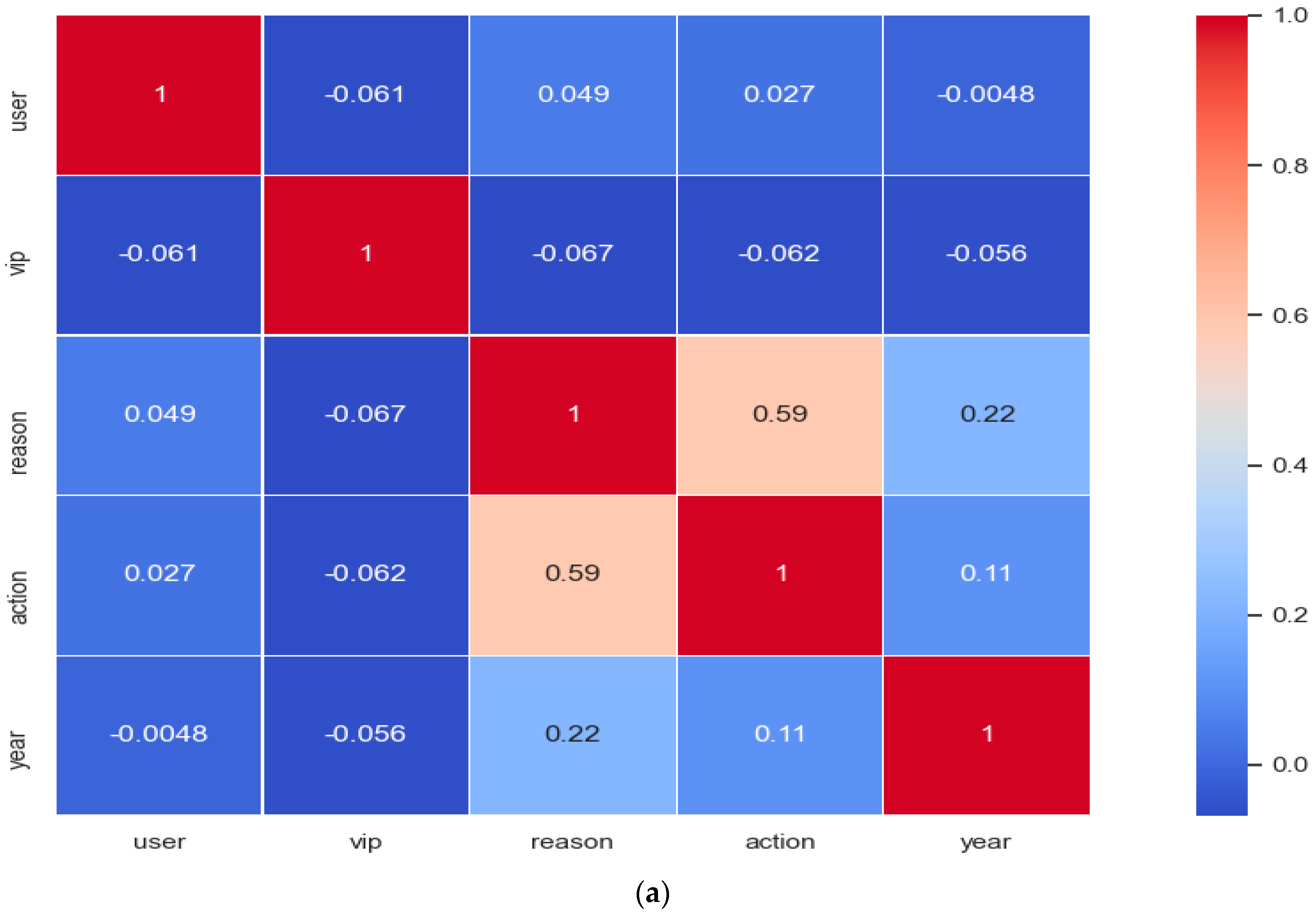
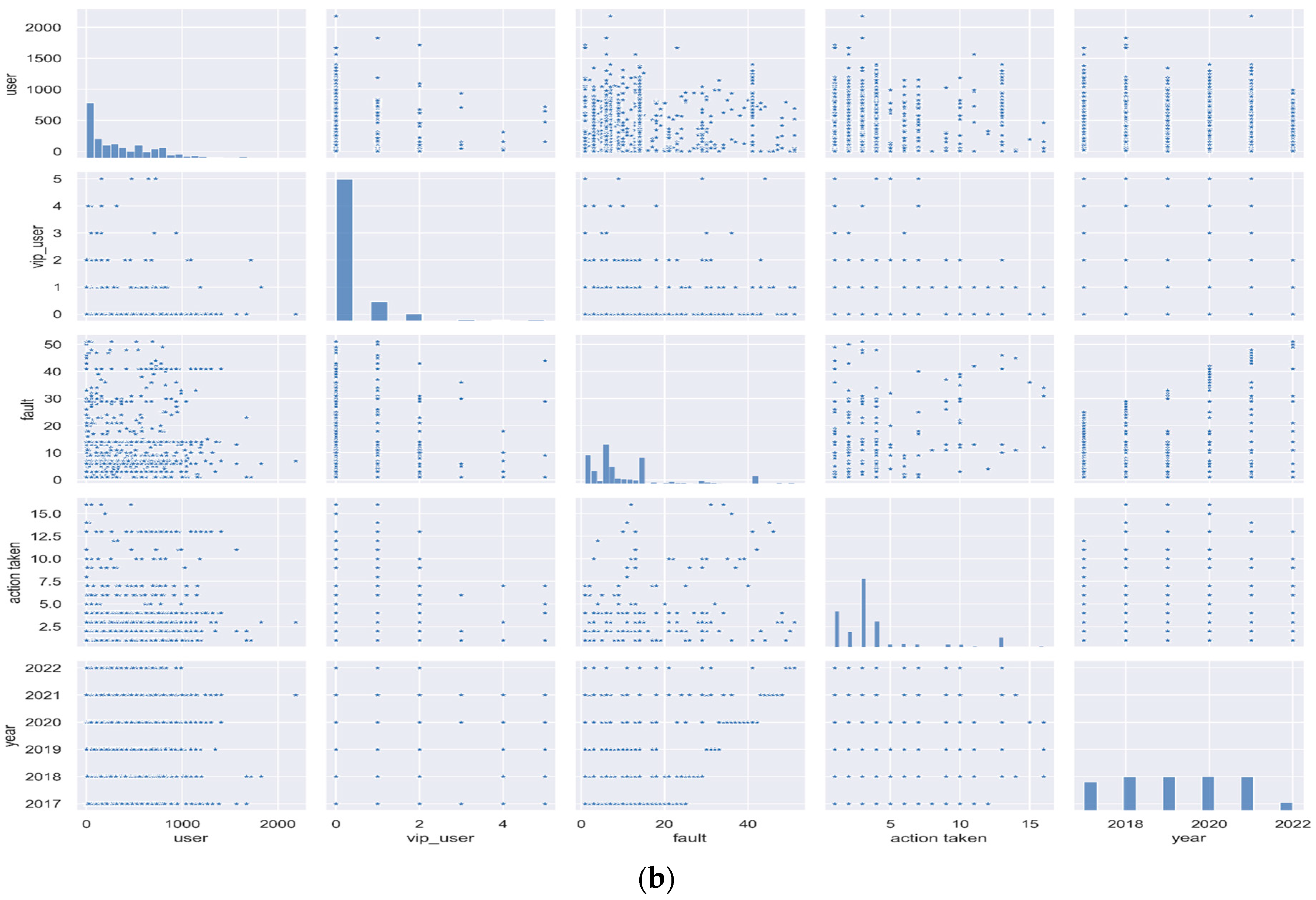
Table 1 shows the classification details of the faults that mostly occurred during the period of 2017–2022 by the users. Similarly, Table 2 lists remedial measures or actions taken against these faults.

2.2. Data Analysis

Figure 2a represents the heat map of the data acquired. This map shows the correlation between the parameters used for forecasting or predicting fault management remedies. The parameters used for the heat map are the number of faults, actions taken against these faults, reasons due to which fault occurred, number of normal and VIP users, and the years during which these faults occurred. The color bar shows the correlation strength between these parameters. Similarly, Figure 2b is the pair plot obtained through data set in which scattered values with respect to other parameters are shown.
Figure 3 shows the box plot of the data parameters, explaining the concentration of the data values. This box plot is categorized into five sections, i.e., users, VIP users, faults that occurred, action taken against each fault, and the number of years. A Box plot is a standardized way to analyze the data, separating it into four equal parts, having 25% each. It tells about the values of the data’s outlier and also shows whether it is symmetrical. In this case, data acquired from the grid station shows that during the first quartile (Q1), the strength of complaints from normal users is very low, but during the second quartile (Q2), 25% of the normal users are below 220. In the third quartile (Q3), 25% of the normal users lie between 220 to 600, and the remaining 25% of users are between 600 to 1400, whereas the strength of VIP users is very low compared to normal users. Similarly, the data is more concentrated in the Q2 during faults, which means 25% of faults occurred between 5 to 7 serial numbers present in Table 2, whereas 25% is from 7 to 15, and the remaining 25% in Q3 are present between 15 to 28 serial numbers as present in Table 2. In the same way, actions taken against these faults are from 1 to 2 during Q1 and 2 to 4 for 50% of the faults during Q2 and Q3. Action or remedial measures from 4 to 7 are taken against the faults that occurred during Q4. Box plots related to the years show that 75% of faults occurred from 2017 to 2020, and the remaining 25% occurred from 2020 to 2022.

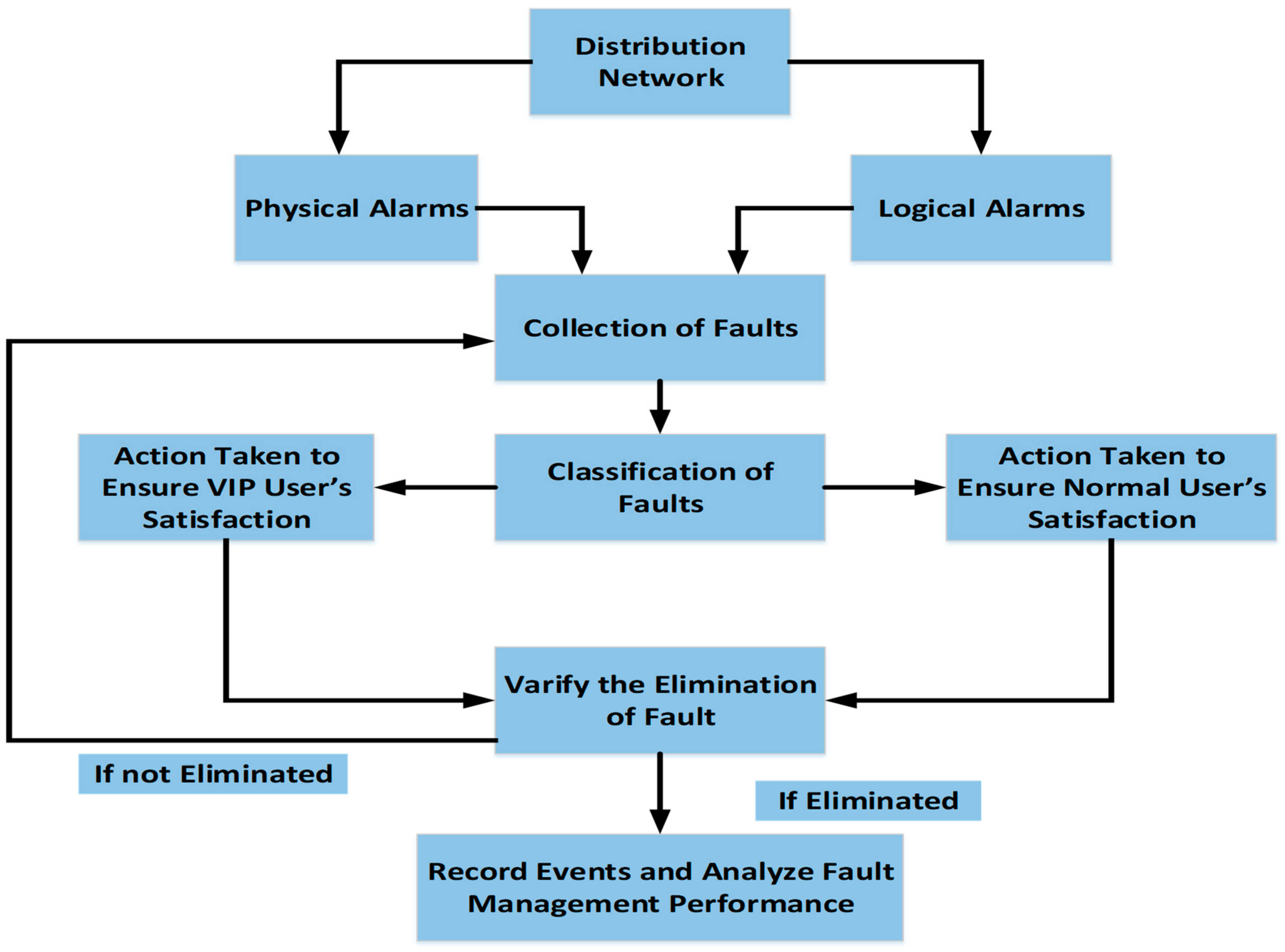
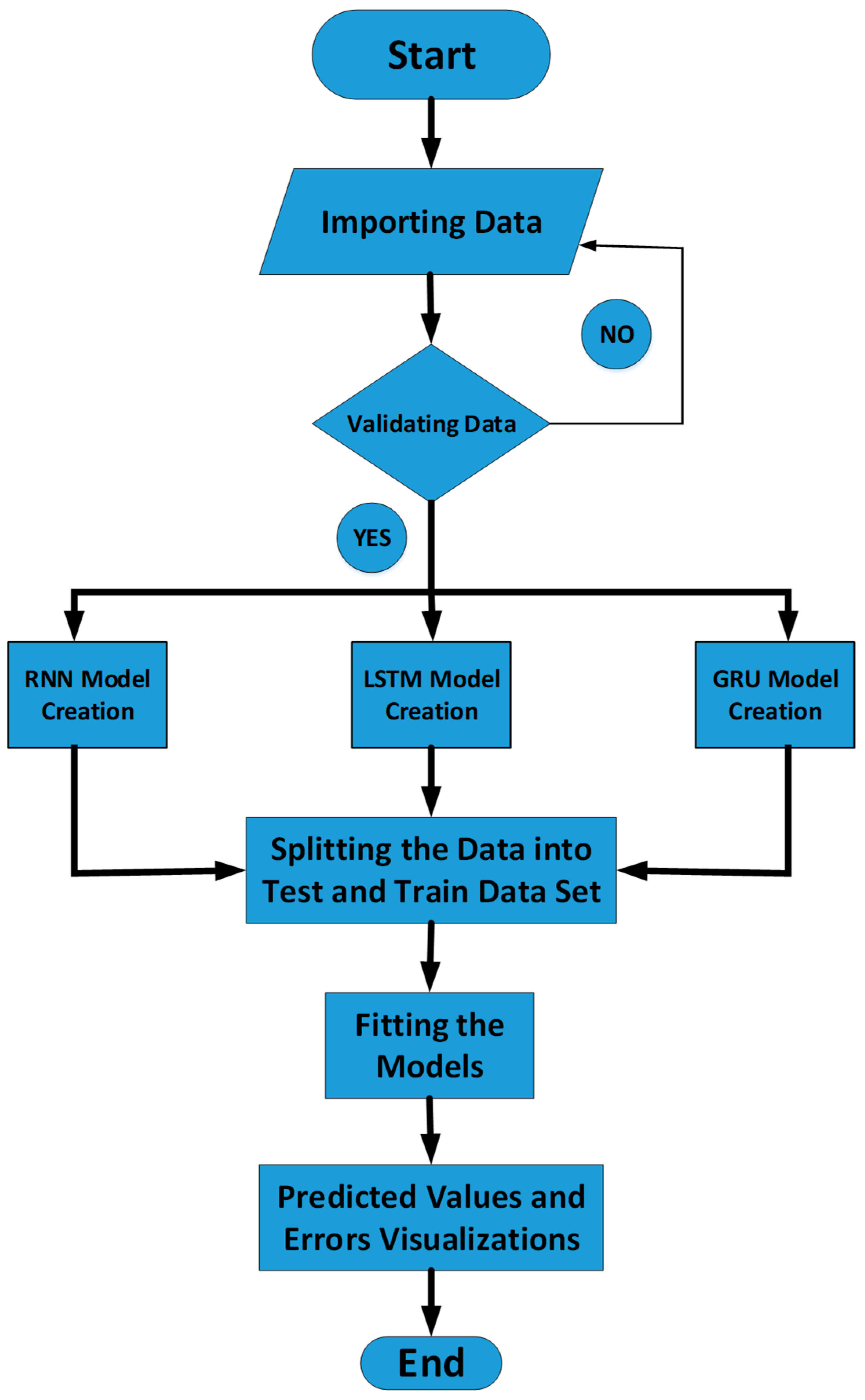
3. Framework with Fault Management

Figure 4 shows a high-level overview of the framework proposed for fault management using deep learning models. The first step of this research is data collection and feature/parameter selection. The second step is partitioning the data, in which 50% training, validating, and 50% testing of the data has been done. After cleaning and testing the data, predicted output result values and projected error values are kept under the models developed after training through 50% of the data. Finally, graphical visualizations have been acquired from these trained models, as shown in Figure 4.
Similarly, the RMS and MAE errors are also tested after training 50% of the data. Again, the graphical visualizations show that the results acquired from the GRU model are much better than the other two methods. Also, the root mean square error (RMSE) loss and mean absolute error loss (MAE) loss for the GRU model is low than that of the LSTM and RNN models.
In a similar manner, Figure 5 depicts the whole process as a flow chart of the procedures involved. Python is used to build and implement the three distinct artificial intelligence strategies, which are recurrent neural networks (RNN), long short-term memory (LSTM), and gate recurrent units (GRU). After the first data set has been imported, an analysis of the state of the data is performed on it, and then it is put through the validation process. During the process of validating the imported data, it is examined to see whether the data ought to be in the form of numbers. This is done because, in time series analysis, the data must not be in the form of strings and must also be legitimate and accurate (no negative numbers, etc.). If the data value is determined to be right or YES, then the process moves on to the next step; otherwise, it is filtered through the validation process once again, as illustrated in the flowchart in Figure 5. The next stage of the procedure involves setting aside half of the data that is being used for training for each of the deep learning RNN, LSTM, and GRU models that have been constructed. After that, it is decided whether the generated model is appropriate for the data that was trained on it. The remaining 50% of the data is used to generate the final set of anticipated values and visualizations. The root mean square errors (RMSE) and the mean absolute errors are shown in this integrated graphical form that shows the final visualization findings (MAE). The comparative study found that the results obtained by the artificial intelligence deep learning model of gate recurrent unit (GRU) for real-time fault classification and the number of users data have a lower percentage of RMSE and MAE values. This was the conclusion reached after comparing the models’ RMSE and MAE values. The following section provides a concise overview of the generated models and their mathematical formulations.

3.1. Mathematical Expressions and Functional Process of RNN, LSTM and GRU

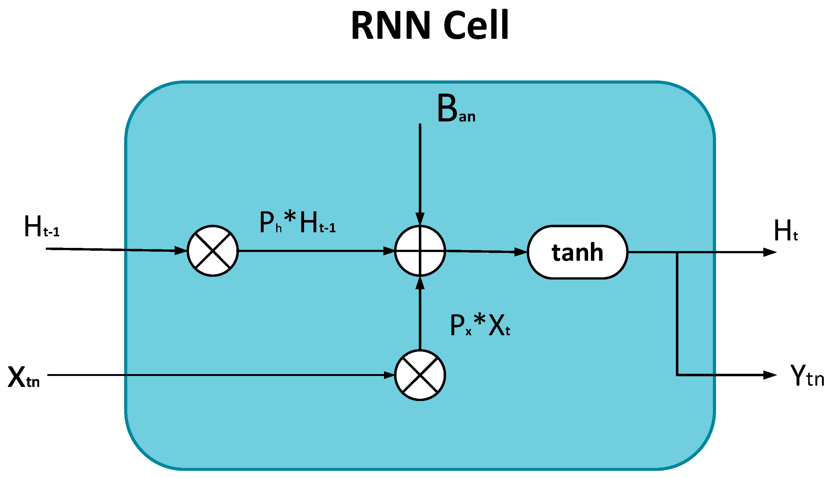
3.1.1. Simple Recurrent Neural Network (RNN)

Elman initially suggested using the recurrent unit as its basic building block (1990). Figure 6 shows the essential composition of an RNN cell. Figure 6 shows the most basic composition of an RNN cell [45].
When used to extremely lengthy sequences, the basic RNN cell has the well-known issues of disappearing gradient and expanding gradient. It is a fact that the basic RNN cells cannot hold long-term dependence in the future. So it is proof that these cells have deficiencies. The back-propagated gradients tend to decrease when the sequences are very lengthy, preventing an effective update of the weights. However, when gradients are substantial, they may erupt across lengthy sequences, rendering weight matrices unstable. Both of these problems stem from the intractable nature of the gradients, making it harder for RNN cells to detect and account for long-term relationships. Equations (1) and (2) show the mathematical expressions for RNN structure [2].
h t 1 = σ ( P h h t 1 + P x x t + B a )
y t = t a n h ( P o h t + B o )
where h t is the hidden state, and it is the only type of memory in the RNN cell. x t and y t represent the input and output of the cell at time step t, respectively. P h and P x are the weight matrices for the hidden state and P o bias vector for the cell output, respectively. B a and B o denote the bias vector for the hidden state and cell output, respectively.
The final hidden state is conditioned on the hidden state of the preceding time step and the current input. The cellular feedback loops that link the present state to the subsequent one support this hypothesis. These bonds are crucial for considering historical data while modifying the current cell state. In this case, the sigmoid function is utilized, denoted by, to turn on the latent state, and the hyperbolic tangent function, denoted by tanh, to turn on the overt state.

3.1.2. GRU Explanation

The GRU is a subset of RNNs. As seen in Figure 7, the GRU differs significantly from the LSTM in that it lacks a cell state and instead employs a simple logic circuit consisting of an update gate ( Z t ) and a reset gate ( R t ), as shown in Figure 7.
They simplify model training as they are a more literal depiction of the LSTM. On the other hand, the GRU is endowed with a hidden state H t that crosses the top of the cell and undergoes periodic updates through a gating mechanism. The GRU requires two inputs, the current input X t and the pre-hidden state H t 1 . These two states are analyzed by two gates that assess whether the information helps modify the hidden state or not. One is the reset gate which decides what percentage of the previous hidden state should be preserved, thereby decreasing the amount of information that can be stored gradually. At first, the current input X t and the prior entry H t 1 are processed through the nonlinear sigmoid function that produces a value between 0 to 1, as illustrated in Equation (3) [2].
R t = σ ( W R H H t 1 + W R X X t )
The second one is the update gate; during the process of the update gate, the input X t and pre-hidden state H t 1 are multiplied by their weights W Z X and W Z H , respectively. These two products are added, and then a sigmoid activation function is utilized, which clamps the output between 0 and 1, as in Equation (4) [2].
Z t = σ ( W Z H H t 1 + W Z X X t )
In Equations (3) and (4), Z t is the output of the reset gate, W R H and W R X represent the weights for the reset gate, W Z H and W Z X represent the weights of the update gate of pre-hidden state H t 1 and input X t , respectively.
Now for H t , the first step is to calculate the product of input X t and its weight W H X . The second step is to find the product of the reset gate ( R t ) and ( H t 1 * W H H ), which will find what value should be remembered or forgotten and then apply the nonlinear function ‘tanh’ by combining these both steps, as in Equation (5) [2].
H t = t a n h { W H H R t H t 1 + W H X X t }
In Equation (5), W H H and W H X are the weight matrix, H t 1 is the pre-hidden state, R t is the reset gate output, X t is the input, and tanh represents the activation function of the output.
During the last stage, an update gate is needed to find what should be collected from the current memory content H t and previous memory content H t 1 . For the update gate, the first step is the product of Z t and H t , and the second step is the product of H t 1 and (1 − Z t ) is needed. By combining these two steps, the value of H t can be determined from the following Equation (6) [2].
H t = t a n h { W H H R t H t 1 + W H X X t }
H t = { 1 Z t H t 1 + Z T H t }
where H t is the final output, H t 1 is the pre-hidden state, R t is the reset gate output in Equation (7) [2].

3.1.3. LSTM Explanation

Long Short Term Memory is a more advanced type of recurrent neural network designed to address issues with explosive and decaying gradients. LSTM, similarly to RNN, is composed of repeated modules; however, the structure is different. Rather than having a single layer of tanh, an LSTM network contains four layers that interact with each other and communicate with one another, as shown in Figure 8. This structure, consisting of three gates or four layers, is useful for LSTM in retaining long-term memory and may be used to address various sequential issues. The internal structure of the LSTM cell is shown in Figure 8.
LSTM cell is divided into three gates. The combined inputs of the hidden state from the preceding time step ( H t 1 ) and the input at the current time step ( X t ) are sent through a series of gates, as shown in Figure 8. The values of H t 1 ) and X t are passed through the sigmoid, which is called forget gate. For gates, the sigmoid function (σ) is used since it returns only positive values and can be relied upon to definitively tell us whether or not a given characteristic should be retained. The sigmoid function has values between 0 and 1, and it determines whether values should be determined, i.e., multiplied with 1 (means gates are open) or forgotten, i.e., multiplied with 0 (means gates are blocked). Equation (8) shows the mathematical expression for the output of forget gate [2].
F t = σ { W F ( H t 1 , X t ) }
Similarly, the input gate is used for determining which factors should be included in the current cell state (C). This gate has two parts; one is the input gate layer having sigmoid. It decides which value should be updated. The other one having a tanh layer constitute new candidate values ( C t ) that could be combined to the state. Equation (9) and Equation (10) represent the input gate parameters [2].
I t = σ { W I ( H t 1 , X t ) }
C t = t a n h { W C H t 1 , X t }
The next process is to update the cell state ( C t ); for this output of the forget gate ( F t ) is multiplied by the previous cell state ( C t 1 , ). Then, the product of the input gate ( I t ) and the cell state candidate’s information ( C t ) is added to get the current cell state ( C t ), as shown in Equation (11) [2].
C t = F t C t 1 + C t C t
The last step of the process is to update the hidden cell. C t is passed through the tanh activation function and then multiplied by the output gate ( O t ) results, as in Equation (12) [2]. In the end, C t and H t move back toward the recurrent unit, Equation (13) [2], and the process starts over at time step t + 1 until it is over, as shown in Figure 8.
O t = σ { W O ( H t 1 , X t ) }
H t = O t tanh C t
where σ is the sigmoid function, It denotes the Input gate, F t is Forget gate, O t , is the output gate, X t is the input at a current Time Step, H t is the hidden state at the current time step, H t 1 , is the hidden state from a previous time step, C t , represents the current cell state, C t signifies a candidate for cell state at the timestamp (t), and C t 1 , is the previous cell state.

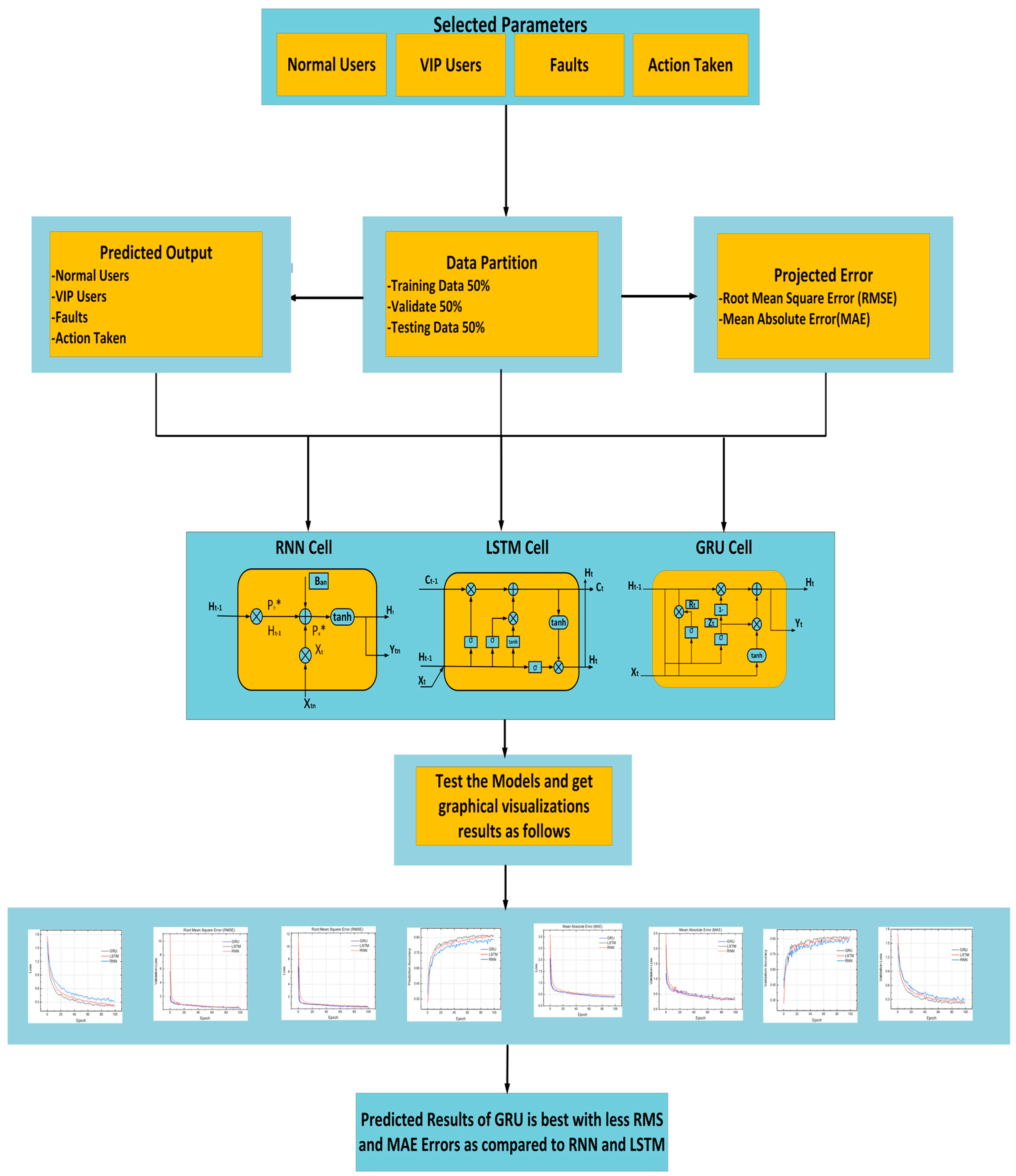
3.1.4. Experimental Setup Used

In this research, the following hardware and software setups were utilized:
  • CPU: Intel(R) Core (TM) i7-10875H [email protected] 2.30 GHz
  • Graphics Card: NVIDIA GeForce RTX 2060
  • RAM: 16.0 GB, 6 GB GUP Memory
  • OS: 64-bit Windows operating system
  • Software: Python 3.7, Keras, TensorFlow version 2.3.1
The resulting handcrafted fused feature set was divided 50:50 across the training and testing sets. Precision, accuracy, recall, and F1-score were standard performance indicators used in assessing results. True Positive (TP), True Negative (TN), False Negative (FN), and False Positive (FP) rates were calculated to determine the value of these standard performance indicators, which are defined as:
  • TP: True positive rate is the number of fault classifications samples that were successfully identified as malignant.
  • TN: True negative rate is the number of benign samples that were successfully identified as benign.
  • FP: False positive rate is the number of benign samples that were wrongly identified as malignant.
  • FN: False negative rate is the number of malignant samples that were wrongly identified as benign.
P r e c i s i o n = T P T P + F P
R e c a l l = F P F P + T N
F 1 S c o r e = 2 × T P T P + F P + F N
A c c u r a c y = T P + T N T P + T N + F P + F N

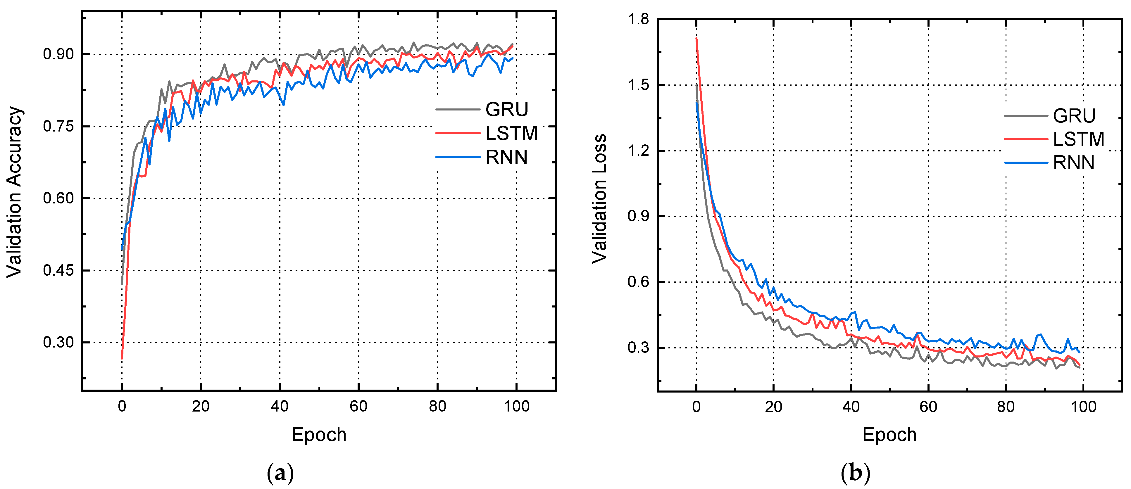
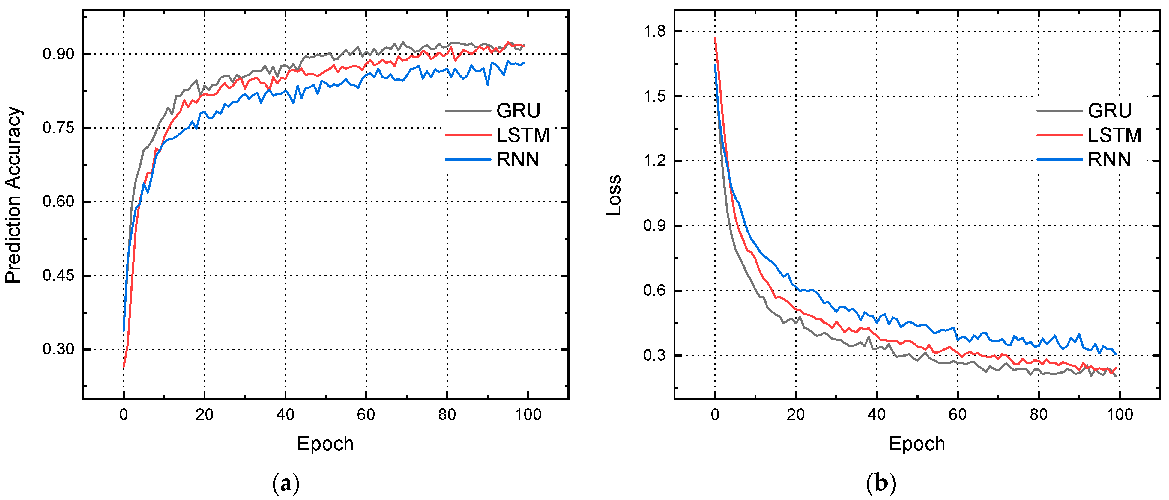
4. Results and Discussion

Figure 9 shows the confusion matrix of the three models used for prediction using the real-time data set of fault classification. A confusion matrix may be used to provide a concise summary of the effectiveness of a categorization system. For example, if there is a considerable imbalance between the quantities of observations in each class or if there are more than two classes in the dataset, placing all of the trust in the classification accuracy alone might be misleading. The confusion matrix also explains the benefits and drawbacks associated with categorization models that are computed. Figure 9a shows the results of the data set in the confusion matrix between the actual values of the data set and values after prediction through the GRU model.
Accurately predicted true positive values from 2017 to 2022 have the highest percentage compared to the values of the other two methods. This means the data is classified as having positive values without the lowest misleading numbers. Similarly, the confusion matrix between actual values of the data set and values after prediction through LSTM and RNN models in Figure 9b and Figure 9c, respectively, show performance results about the data. However, it can be clearly seen that GRU is showing better results than LSTM and RNN. At the same time, RNN performed poorly than the other two methods.
Figure 10 compares the RMSE validation loss graph of the models designed and the RMSE loss after prediction by using 100 epochs on the x-axis. It is observed in Figure 10a that validation loss through RNN starts after the first epoch and from 10 on the y-axis and suddenly decreases. After that, the fluctuation can be seen until the last epoch. In the same way, validation loss in GRU and LSTM is less than RNN and starts from 5.5, then decreases and continuously remains to fluctuate up to the 100th epoch. If the validation results of RMSE loss compare with the predicted RMSE loss, then it can be clearly seen here that GRU is giving much better results than LSTM and RNN as the RMSE loss of GRU in prediction is very low.
Figure 11 shows the comparison between the mean absolute error (MAE) validation loss graph of the models designed and the MAE loss after prediction using 100 epochs on the x-axis. It can be seen in Figure 11a that validation loss through RNN starts to decline from zero, and after the first epoch, a gradual fluctuating decrease can be seen until the last epoch. In the same way, validation loss in GRU and LSTM is less than RNN and starts from 1.5, then decreases and continuously remains to fluctuate up to the 100th epoch. If the validation results of MAE loss compare with the predicted MAE loss, it can be clearly seen that GRU is performing much better than LSTM and RNN as the MAE loss of GRU is very low.
After training 50% of the data, validation accuracy and loss of the three models are determined through graphical visualization in Figure 12a,b. Figure 12a shows that the validation accuracy of the GRU model starts from 0.45 at the start, then goes on increasing up to 0.93 and remains constant till the 100th epoch, which is higher than the LSTM and RNN validation accuracy. In contrast, the Validation loss of GRU is much lower than that of LSTM and RNN as it starts from 1.4 and decreases down to 0.2, as shown in Figure 12b compared to the losses of LSTM and RNN models. On the other hand, the highest validation loss is from the RNN model, starting from 1.7 and decreasing to 0.39 until the last epoch, as in Figure 12b.
In Figure 13, prediction accuracy and prediction loss are described in graphical visualization form. Figure 13a shows that the accuracy of the model GRU is more than that of LSTM and RNN. Similarly, in the same way, the GRU loss in Figure 13b is the lowest compared to the other two models. The prediction accuracy of GRU starts from 0.5 and increases up to 0.93, whereas its loss is from 1.4 to a minimum value of 0.28. The model RNN shows the lowest performance in both, i.e., prediction accuracy and loss.
Table 3, Table 4 and Table 5 below summarize the trainable and non-trainable parameters of the data forecasting framework for the GRU, LSTM, and RNN, respectively. This is done after the datasets have been divided into training, validation, and testing sets and the appropriate fine-tuned parameters have been selected. The results of employing gradients to update the values of trainable parameters, such as error, loss, and cost relative to chosen hyperparameters in neural networks, are shown in Table 3, Table 4 and Table 5 indicate that there are over 394,758 trainable parameters for GRU, over 524,358 trainable parameters for LSTM, and over 131,238 trainable parameters for RNN. A model’s accuracy could improve with more trainable parameters, but this comes with a greater danger of overfitting. Dropout layers were included in the model to prevent the overfitting and underfitting that plague neural networks. Tensor Flow and Keras may show overfitting and underfitting due to tunable parameters by plotting epochs versus training and validation losses. A model is considered underfitting if it does not increase its performance on either the training or validation sets. It is claimed that a model is overfitting if, despite prolonged training, it still performs poorly on the validation set. One indicator of a well-fitting model is its ability to perform well not just on the training set but also on the validation set, a phenomenon known as transfer learning. In order to assess whether the suggested neural network model’s parameters are indeed trainable, one might look at epoch curves depicting training and validation loss.
Table 6 discusses the resulting overall summary of all predicted models. It can be seen that the losses of RNN and LSTM are 0.28 and 0.22, respectively, whereas the loss of GRU is lower than both of them. Similarly, the accuracy of GRU is higher than RNN and LSTM, which is 92.13%. In the same way, the MAE and RMSE loss of GRU is 0.37 and 0.39, which is the lowest among all three models.

5. Conclusions

Since traditional secondary techniques often lack fault monitoring and normalization systems, resolving power outage concerns in distribution networks is a time-consuming and complex task. Distribution network operators have a significant challenge in fault management. Systems that can go through the deluge of incoming data, diagnose problems, and suggest fixes may take a massive load off the operator’s shoulders. In this research, some AI neural network models are available for defect prediction and how to fix them, including GRUs, LSTMs, and RNNs. After training and testing the models, predictions and forecasts were made using real-time data on physical and logical faults occurring at Tabuk grid station from 2017 to 2022. Graphical representations generated allowed for a comparison of results, showing that GRU outperformed LSTM and RNN. The overall analysis revealed that GRU achieved a prediction performance of over 90% with a prediction loss of less than 20%. Similarly, it was evident from the results that RMSE and MAE loss of GRU (both validation and prediction) was lower than that of LSTM and RNN. Compared to LSTM (91.69%) and RNN (81.21%), GRU’s accuracy is much higher at 92.13%. For this reason, the fault management system of today and the future will benefit from the incorporation of AI methods or models that will allow for more nuanced and accurate diagnoses of problems and the implementation of appropriate corrective measures. In future, some latest AI techniques will be implemented for enhancing the response towards any fault occurred with in or out of the grid system. For making the system more swift and efficient for the users and for the service providers, ensemble will be developed through different artificial intelligence models like LSTM, AdaBoost, XGBoost, etc.

Funding

This research received no external funding.

Data Availability Statement

Data is unavailable due to privacy.

Conflicts of Interest

The authors declare no conflict of interest.

References

  1. US DOE. Enabling modernization of the electric power system. In Quadrennial Technology Review; US DOE: Washington, DC, USA, 2015; Volume 22. [Google Scholar]
  2. Abubakar, M.; Che, Y.; Ivascu, L.; Almasoudi, F.M.; Jamil, I. Performance Analysis of Energy Production of Large-Scale Solar Plants Based on Artificial Intelligence (Machine Learning) Technique. Processes 2022, 10, 1843. [Google Scholar] [CrossRef]
  3. Sarfraz, M.; Naseem, S.; Mohsin, M.; Bhutta, M.S.; Jaffri, Z.U.A.; Chen, C.; Zhang, Z.; Wei, L.; Qiu, Y.; Xu, W.; et al. Recent analytical tools to mitigate carbon-based pollution: New insights by using wavelet coherence for a sustainable environment. Environ. Res. 2022, 212, 113074. [Google Scholar] [CrossRef]
  4. Sarfraz, M.; Iqbal, K.; Wang, Y.; Bhutta, M.S.; Jaffri, Z.U.A. Role of agricultural resource sector in environmental emissions and its explicit relationship with sustainable development: Evidence from agri-food system in China. Resour. Policy 2023, 80, 103191. [Google Scholar] [CrossRef]
  5. Bhutta, M.S.; Sarfraz, M.; Ivascu, L.; Li, H.; Rasool, G.; Jaffri, Z.U.A.; Farooq, U.; Shaikh, J.A.; Nazir, M.S. Voltage Stability Index Using New Single-Port Equivalent Based on Component Peculiarity and Sensitivity Persistence. Processes 2021, 9, 1849. [Google Scholar] [CrossRef]
  6. Chen, W.; Liu, B.; Nazir, M.S.; Abdalla, A.N.; Mohamed, M.A.; Ding, Z.; Bhutta, M.S.; Gul, M. An Energy Storage Assessment: Using Frequency Modulation Approach to Capture Optimal Coordination. Sustainability 2022, 14, 8510. [Google Scholar] [CrossRef]
  7. Nazir, M.S.; Abdalla, A.N.; Zhao, H.; Chu, Z.; Nazir, H.M.J.; Bhutta, M.S.; Javed, M.S.; Sanjeevikumar, P. Optimized economic operation of energy storage integration using improved gravitational search algorithm and dual stage optimization. J. Energy Storage 2022, 50, 104591. [Google Scholar] [CrossRef]
  8. Mnyanghwalo, D.; Kawambwa, S.; Mwifunyi, R.; Gilbert, G.M.; Makota, D.; Mvungi, N. Fault Detection and Monitoring in Secondary Electric Distribution Network Based on Distributed Processing. In Proceedings of the 2018 Twentieth International Middle East Power Systems Conference (MEPCON), Cairo, Egypt, 18–20 December 2018; pp. 84–89. [Google Scholar] [CrossRef]
  9. Jamil, M.; Sharma, S.K.; Singh, R. Fault detection and classification in electrical power transmission system using artificial neural network. SpringerPlus 2015, 4, 334. [Google Scholar] [CrossRef] [Green Version]
  10. Kaur, K.; Kaur, R. Energy management system using PLC and SCADA. Int. J. Eng. Res. Technol. 2014, 3, 528–531. [Google Scholar]
  11. Gou, B.; Kavasseri, R.G. Unified PMU Placement for Observability and Bad Data Detection in State Estimation. IEEE Trans. Power Syst. 2014, 29, 2573–2580. [Google Scholar] [CrossRef]
  12. Shahriar, M.S.; Habiballah, I.O.; Hussein, H. Optimization of Phasor Measurement Unit (PMU) Placement in Supervisory Control and Data Acquisition (SCADA)-Based Power System for Better State-Estimation Performance. Energies 2018, 11, 570. [Google Scholar] [CrossRef]
  13. Motlagh, N.H.; Mohammadrezaei, M.; Hunt, J.; Zakeri, B. Internet of Things (IoT) and the Energy Sector. Energies 2020, 13, 494. [Google Scholar] [CrossRef] [Green Version]
  14. Wani, S.A.; Rana, A.S.; Sohail, S.; Rahman, O.; Parveen, S.; Khan, S.A. Advances in DGA based condition monitoring of transformers: A review. Renew. Sustain. Energy Rev. 2021, 149, 111347. [Google Scholar] [CrossRef]
  15. Duan, H.; Liu, D. Application of improved Elman neural network based on fuzzy input for fault diagnosis in oil-filled power transformers. In Proceedings of the 2011 International Conference on Mechatronic Science, Electric Engineering and Computer (MEC), Jilin, China, 19–22 August 2011; pp. 28–31. [Google Scholar]
  16. Wang, F.; Bi, J.; Zhang, B.; Yuan, S. Research of Transformer Intelligent Evaluation and Diagnosis Method Based on DGA. MATEC Web Conf. 2016, 77, 01002. [Google Scholar] [CrossRef] [Green Version]
  17. Qi, B.; Wang, Y.; Zhang, P.; Li, C.; Wang, H. A Novel Deep Recurrent Belief Network Model for Trend Prediction of Transformer DGA Data. IEEE Access 2019, 7, 80069–80078. [Google Scholar] [CrossRef]
  18. Yan, C.; Li, M.; Liu, W. Transformer Fault Diagnosis Based on BP-Adaboost and PNN Series Connection. Math. Probl. Eng. 2019, 2019, 1019845. [Google Scholar] [CrossRef] [Green Version]
  19. Yang, X.; Chen, W.; Li, A.; Yang, C.; Xie, Z.; Dong, H. BA-PNN-based methods for power transformer fault diagnosis. Adv. Eng. Inform. 2019, 39, 178–185. [Google Scholar] [CrossRef]
  20. Yang, X.; Chen, W.; Li, A.; Yang, C. A Hybrid machine-learning method for oil-immersed power transformer fault diagnosis. IEEJ Trans. Electr. Electron. Eng. 2019, 15, 501–507. [Google Scholar] [CrossRef]
  21. Luo, Z.; Zhang, Z.; Yan, X.; Qin, J.; Zhu, Z.; Wang, H.; Gao, Z. Dissolved Gas Analysis of Insulating Oil in Electric Power Transformers: A Case Study Using SDAE-LSTM. Math. Probl. Eng. 2020, 2020, 2420456. [Google Scholar] [CrossRef]
  22. Velásquez, R.M.A.; Lara, J.V.M. Root cause analysis improved with machine learning for failure analysis in power transformers. Eng. Fail. Anal. 2020, 115, 104684. [Google Scholar] [CrossRef]
  23. Mi, X.; Subramani, G.; Chan, M. The Application of RBF Neural Network Optimized by K-means and Genetic-backpropagation in Fault Diagnosis of Power Transformer. E3S Web Conf. 2021, 242, 03002. [Google Scholar] [CrossRef]
  24. Taha, I.B.M.; Ibrahim, S.; Mansour, D.-E.A. Power Transformer Fault Diagnosis Based on DGA Using a Convolutional Neural Network with Noise in Measurements. IEEE Access 2021, 9, 111162–111170. [Google Scholar] [CrossRef]
  25. Zhou, Y.; Yang, X.; Tao, L.; Yang, L. Transformer Fault Diagnosis Model Based on Improved Gray Wolf Optimizer and Probabilistic Neural Network. Energies 2021, 14, 3029. [Google Scholar] [CrossRef]
  26. Wang, Y.; Zhang, L. A Combined Fault Diagnosis Method for Power Transformer in Big Data Environment. Math. Probl. Eng. 2017, 2017, 9670290. [Google Scholar] [CrossRef] [Green Version]
  27. Fang, J.; Zheng, H.; Liu, J.; Zhao, J.; Zhang, Y.; Wang, K. A Transformer Fault Diagnosis Model Using an Optimal Hybrid Dissolved Gas Analysis Features Subset with Improved Social Group Optimization-Support Vector Machine Classifier. Energies 2018, 11, 1922. [Google Scholar] [CrossRef] [Green Version]
  28. Huang, X.; Zhang, Y.; Liu, J.; Zheng, H.; Wang, K. A Novel Fault Diagnosis System on Polymer Insulation of Power Transformers Based on 3-stage GA–SA–SVM OFC Selection and ABC–SVM Classifier. Polymers 2018, 10, 1096. [Google Scholar] [CrossRef] [Green Version]
  29. Illias, H.A.; Liang, W.Z. Identification of transformer fault based on dissolved gas analysis using hybrid support vector machine-modified evolutionary particle swarm optimisation. PLoS ONE 2018, 13, e0191366. [Google Scholar] [CrossRef] [Green Version]
  30. Kari, T.; Gao, W.; Zhao, D.; Abiderexiti, K.; Mo, W.; Wang, Y.; Luan, L. Hybrid feature selection approach for power transformer fault diagnosis based on support vector machine and genetic algorithm. IET Gener. Transm. Distrib. 2018, 12, 5672–5680. [Google Scholar] [CrossRef]
  31. Kim, Y.; Park, T.; Kim, S.; Kwak, N.; Kweon, D. Artificial Intelligent Fault Diagnostic Method for Power Transformers using a New Classification System of Faults. J. Electr. Eng. Technol. 2019, 14, 825–831. [Google Scholar] [CrossRef]
  32. Zeng, B.; Guo, J.; Zhu, W.; Xiao, Z.; Yuan, F.; Huang, S. A Transformer Fault Diagnosis Model Based on Hybrid Grey Wolf Optimizer and LS-SVM. Energies 2019, 12, 4170. [Google Scholar] [CrossRef] [Green Version]
  33. Zhang, Y.; Li, X.; Zheng, H.; Yao, H.; Liu, J.; Zhang, C.; Peng, H.; Jiao, J. A Fault Diagnosis Model of Power Transformers Based on Dissolved Gas Analysis Features Selection and Improved Krill Herd Algorithm Optimized Support Vector Machine. IEEE Access 2019, 7, 102803–102811. [Google Scholar] [CrossRef]
  34. Zhang, Y.; Wang, Y.; Fan, X.; Zhang, W.; Zhuo, R.; Hao, J.; Shi, Z. An Integrated Model for Transformer Fault Diagnosis to Improve Sample Classification near Decision Boundary of Support Vector Machine. Energies 2020, 13, 6678. [Google Scholar] [CrossRef]
  35. Benmahamed, Y.; Kherif, O.; Teguar, M.; Boubakeur, A.; Ghoneim, S. Accuracy Improvement of Transformer Faults Diagnostic Based on DGA Data Using SVM-BA Classifier. Energies 2021, 14, 2970. [Google Scholar] [CrossRef]
  36. Islam, M.; Lee, G.; Hettiwatte, S.N. A nearest neighbour clustering approach for incipient fault diagnosis of power transformers. Electr. Eng. 2017, 99, 1109–1119. [Google Scholar] [CrossRef]
  37. Li, E.; Wang, L.; Song, B.; Jian, S. Improved Fuzzy C-Means Clustering for Transformer Fault Diagnosis Using Dissolved Gas Analysis Data. Energies 2018, 11, 2344. [Google Scholar] [CrossRef] [Green Version]
  38. Misbahulmunir, S.; Ramachandaramurthy, V.K.; Thayoob, Y.H.M. Improved Self-Organizing Map Clustering of Power Transformer Dissolved Gas Analysis Using Inputs Pre-Processing. IEEE Access 2020, 8, 71798–71811. [Google Scholar] [CrossRef]
  39. Elsheikh, A.H.; Sharshir, S.W.; Elaziz, M.A.; Kabeel, A.; Guilan, W.; Haiou, Z. Modeling of solar energy systems using artificial neural network: A comprehensive review. Sol. Energy 2019, 180, 622–639. [Google Scholar] [CrossRef]
  40. Elsheikh, A.H.; Saba, A.I.; Panchal, H.; Shanmugan, S.; Alsaleh, N.A.; Ahmadein, M. Artificial Intelligence for Forecasting the Prevalence of COVID-19 Pandemic: An Overview. Healthcare 2021, 9, 1614. [Google Scholar] [CrossRef]
  41. Elsheikh, A. Bistable Morphing Composites for Energy-Harvesting Applications. Polymers 2022, 14, 1893. [Google Scholar] [CrossRef]
  42. Moustafa, E.B.; Elsheikh, A. Predicting Characteristics of Dissimilar Laser Welded Polymeric Joints Using a Multi-Layer Perceptrons Model Coupled with Archimedes Optimizer. Polymers 2023, 15, 233. [Google Scholar] [CrossRef]
  43. Elsheikh, A.H.; Elaziz, M.A.; Vendan, A. Modeling ultrasonic welding of polymers using an optimized artificial intelligence model using a gradient-based optimizer. Weld. World 2021, 66, 27–44. [Google Scholar] [CrossRef]
  44. AbuShanab, W.S.; Elaziz, M.A.; Ghandourah, E.I.; Moustafa, E.B.; Elsheikh, A.H. A new fine-tuned random vector functional link model using Hunger games search optimizer for modeling friction stir welding process of polymeric materials. J. Mater. Res. Technol. 2021, 14, 1482–1493. [Google Scholar] [CrossRef]
  45. Elsheikh, A.H.; Elaziz, M.A.; Das, S.R.; Muthuramalingam, T.; Lu, S. A new optimized predictive model based on political optimizer for eco-friendly MQL-turning of AISI 4340 alloy with nano-lubricants. J. Manuf. Process. 2021, 67, 562–578. [Google Scholar] [CrossRef]
  46. Moustafa, E.B.; Hammad, A.H.; Elsheikh, A.H. A new optimized artificial neural network model to predict thermal efficiency and water yield of tubular solar still. Case Stud. Therm. Eng. 2021, 30, 101750. [Google Scholar] [CrossRef]
  47. Khoshaim, A.B.; Moustafa, E.B.; Bafakeeh, O.T.; Elsheikh, A.H. An Optimized Multilayer Perceptrons Model Using Grey Wolf Optimizer to Predict Mechanical and Microstructural Properties of Friction Stir Processed Aluminum Alloy Reinforced by Nanoparticles. Coatings 2021, 11, 1476. [Google Scholar] [CrossRef]
  48. Elsheikh, A.H.; Katekar, V.P.; Muskens, O.L.; Deshmukh, S.S.; Elaziz, M.A.; Dabour, S.M. Utilization of LSTM neural network for water production forecasting of a stepped solar still with a corrugated absorber plate. Process Saf. Environ. Prot. 2020, 148, 273–282. [Google Scholar] [CrossRef]
  49. DiPietro, R.; Hager, G.D. Chapter 21—Deep learning: RNNs and LSTM. In Handbook of Medical Image Computing and Computer Assisted Intervention; Zhou, S.K., Rueckert, D., Fichtinger, G., Eds.; The Elsevier and MICCAI Society Book Series; Academic Press: Cambridge, MA, USA, 2020; pp. 503–519. ISBN 9780128161760. [Google Scholar] [CrossRef]
Figure 1. Data collection and classification of faults diagram.
Energies 16 01026 g001
Figure 2. (a) Heat map of the data collected from Tabuk grid station; (b) Pair plot of the data collected from Tabuk grid station.
Energies 16 01026 g002aEnergies 16 01026 g002b
Figure 3. Box plot of the data collected from Tabuk grid station.
Energies 16 01026 g003
Figure 4. Proposed framework to find the best model for Fault Management Perdition.
Energies 16 01026 g004
Figure 5. Procedural flow chart to find predicted values.
Energies 16 01026 g005
Figure 6. RNN internal structure.
Energies 16 01026 g006
Figure 7. Internal structure of GRU.
Energies 16 01026 g007
Figure 8. Internal structure of LSTM.
Energies 16 01026 g008
Figure 9. Confusion matrix through (a) GRU, (b) LSTM, and (c) RNN.
Energies 16 01026 g009
Figure 10. (a) RMSE validation loss through GRU, LSTM and RNN; (b) actual predicted RMSE Loss through GRU, LSTM and RNN.
Energies 16 01026 g010
Figure 11. (a) MAE validation loss through GRU, LSTM and RNN; (b) Actual predicted MAE loss through GRU, LSTM and RNN.
Energies 16 01026 g011
Figure 12. (a) Validation Accuracy of the developed models GRU, LSTM and RNN; (b) Validation Loss of the developed models GRU, LSTM and RNN.
Energies 16 01026 g012
Figure 13. (a) Prediction accuracy of the models GRU, LSTM and RNN after testing 50% data; (b) Prediction loss of the models GRU, LSTM and RNN after testing 50% data.
Energies 16 01026 g013
Table 1. Types of faults occurred during the period of 2017–2020.
No.Outage Reason
1Breakdown-Failure
2Contact with conductors (birds/animals)
3End connection combustion (to-ring/ crank unit)
4Shaft / tensioner / bracket damaged by an external factor
5Power cut due to (sandstorm/wind)
6Straightening/T-joint failure
7Cable failure caused by an external factor
8Power cut due to (rain/thunderstorm)
9Force majeure (disasters, floods, earthquakes)
10Separation due to transmission protection
11Disconnection of the feeder due to a fault in the subscriber’s network
12broken insulation
13Emergency separation
14Cable failure due to (longevity/insulation defect)
15power restored to the feeder with a fault that has not been isolated
16Blowout / air breaker switch (LBS) failure
17Throw wires and metal pieces at the connectors
18contact with conductors (trees)
19Wrong operation of the protection devices
20antenna transducer failure
21Failure of the cable connection with the antenna connector
22Detachable / burning jumper
23A pillar fell due to the wind
24Feeder breaker end combustion
25Separation of the feeder at the request of the Civil Defense Department
26Disconnection of the circuit breaker for the senior subscribers’ switching unit due to a fault in the subscriber’s network
27Distribution substation transformer failure (compact / unit / building)
28Damage to the splicing unit (annular/expandable) by an external factor
29Transformer end connection combustion
30Internal failure of the toroidal wrench
31Earth transformer failure without toroidal unit
32Ground transformer combustion without toroidal unit
33Part/or the entire main distribution station is out of service
34Distribution substation transformer combustion (compact/unit/building)
35Failure of the lightning rod
36Failure due to feeder overload
37Internal combustion of the VIP subscribers switch unit
38Emergency break for overhead jumper repair
39Cut / rupture of the antenna connector
40Emergency disconnection at the request of the civil defense / government agency
41Failure due to transmission network
42Emergency disconnection for operational operations (transfer or reload/ failure isolation/ change (N.O)
43Key failure caused by an animal
44one of the phases touches another phase
45Emergency disconnection at the request of the subscriber
46Emergency disconnection at the request of other activities (transmission – power plant)
47Transformer damage by external factor
48Failure of the GIS circuit breaker end connection
49Failure of the protection system
50A main distribution station breaker failure due to a fault in the trip setting values
Table 2. Remedial measures or action taken against the faults.
No.Action Taken
1Turned on and back to normal
2Isolated and restarted from alternate source
3Isolated and gradual restart
4Isolated and restarted
5Replaced and restarted
6Restarted after passing the overhead line
7Eliminated and restarted
8Isolated and waiting for the subscriber to fix the fault
9The subscriber has been isolated and restarted
10Repaired and restarted
11The isolation point has been changed and restarted
12After checking, the switch was turned off and restarted
13After approval from the transmission network, it was restarted
14Restarted after the subscriber fixed the failure
15Loads reduced and restarted
Table 3. Summary of model parameters based on fine-tuned GRU neural network.
Layer (Type)Output ShapeParam #
gru (GRU)(None, None, 256)199,680
dropout (Dropout)(None, None, 256)0
gru_1 (GRU)(None, None, 128)148,224
dropout_1 (Dropout)(None, None, 128)0
gru_2 (GRU)(None, None, 64)37,248
dropout_2 (Dropout)(None, None, 64)0
gru_3 (GRU)(None, 32)9408
dropout_3 (Dropout)(None, 32)0
dense (Dense)(None, 6)198
activation (Activation)(None, 6)0
Total params 394,758
Trainable params 394,758
Non-trainable params 0
Performance of GRU
Loss: 0.21, Accuracy: 92.13%
# Number of parameters
Table 4. Summary of model parameters based on fine-tuned LSTM neural network.
Layer (Type)Output ShapeParam #
lstm (LSTM)(None, None, 256)265,216
dropout (Dropout)(None, None, 256)0
lstm_1 (LSTM)(None, None, 128)197,120
dropout_1 (Dropout)(None, None, 128)0
lstm_2 (LSTM)(None, None, 64)49,408
dropout_2 (Dropout)(None, None, 64)0
lstm_3 (LSTM)(None, 32)12,416
dropout_3 (Dropout)(None, 32)0
dense (Dense)(None, 6)198
activation (Activation)(None, 6)0
Total params 524,358
Trainable params 524,358
Non-trainable params 0
Performance of LSTM
Loss: 0.22, Accuracy:91.69%
# Number of parameters
Table 5. Summary of model parameters based on fine-tuned RNN neural network.
Layer (Type)Output ShapeParam #
simple_rnn (SimpleRNN)(None, None, 256)66304
dropout (Dropout)(None, None, 256)0
simple_rnn_1 (SimpleRNN)(None, None, 128)49280
dropout_1 (Dropout)(None, None, 128)0
simple_rnn_2 (SimpleRNN)(None, None, 64)12352
dropout_2 (Dropout)(None, None, 64)0
simple_rnn_3 (SimpleRNN)(None, 32)3104
dropout_3 (Dropout)(None, 32)0
dense (Dense)(None, 6)198
activation (Activation)(None, 6)0
Total params 131,238
Trainable params 131,238
Non-trainable params 0
Performance of Simple RNN
Loss: 0.28, Accuracy: 89.21%
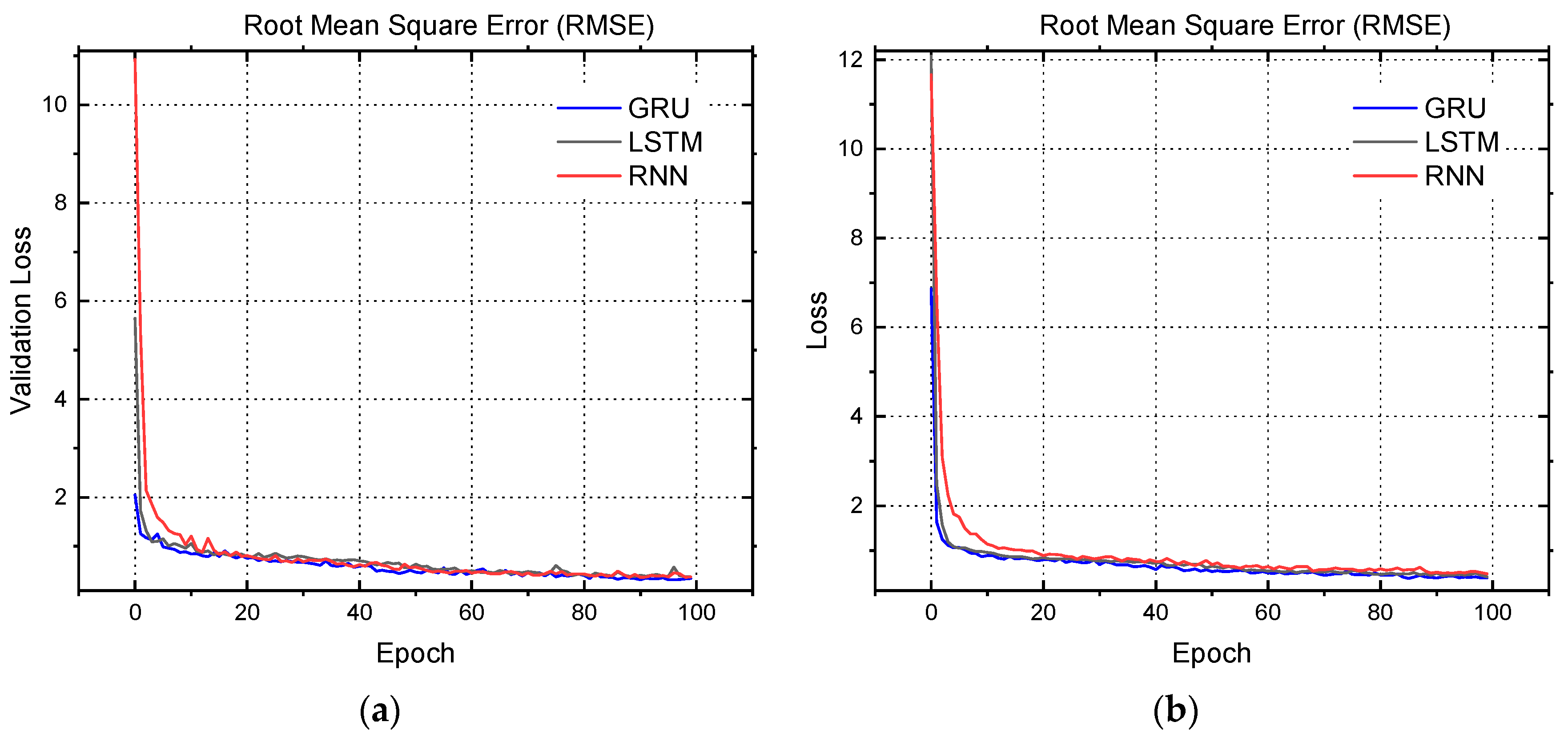
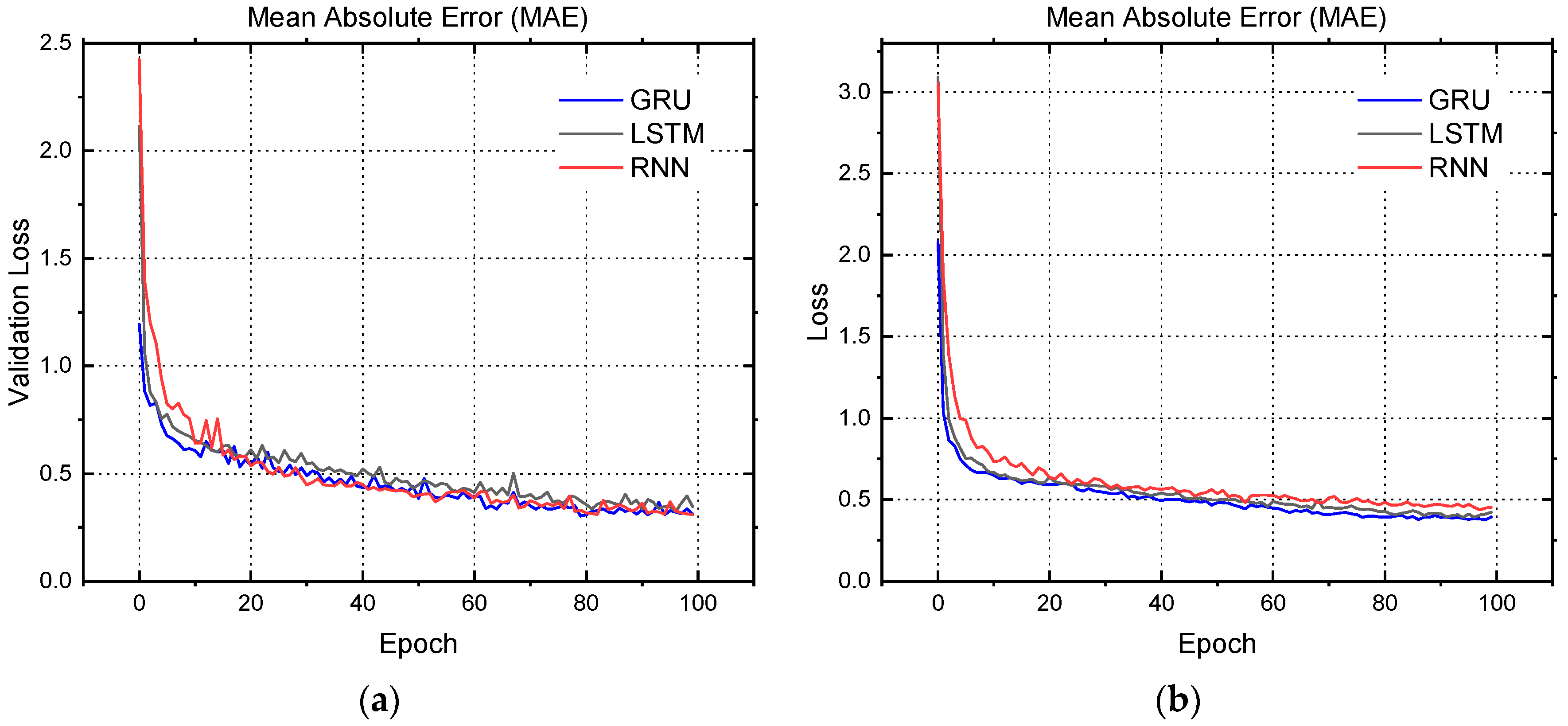
# Number of parameters
Table 6. Performance evaluation of various neural network models in terms of losses and accuracy.
Model of Neural Network PredictionLossesAccuracy (%)MAE LossRMSE Loss
Recurrent Neural Network (RNN)0.2889.210.450.47
Long-Short Term Memory (LSTM)0.2291.690.420.40
Gated Recurrent Unit (GRU)0.2192.130.370.39
Disclaimer/Publisher’s Note: The statements, opinions and data contained in all publications are solely those of the individual author(s) and contributor(s) and not of MDPI and/or the editor(s). MDPI and/or the editor(s) disclaim responsibility for any injury to people or property resulting from any ideas, methods, instructions or products referred to in the content.

