
Hardware-in-the-Loop Testing for Protective Relays Using Real Time Digital Simulator (RTDS)


Abstract
:1. Introduction
2. Development of a RTDS Model for the Five-Bus System
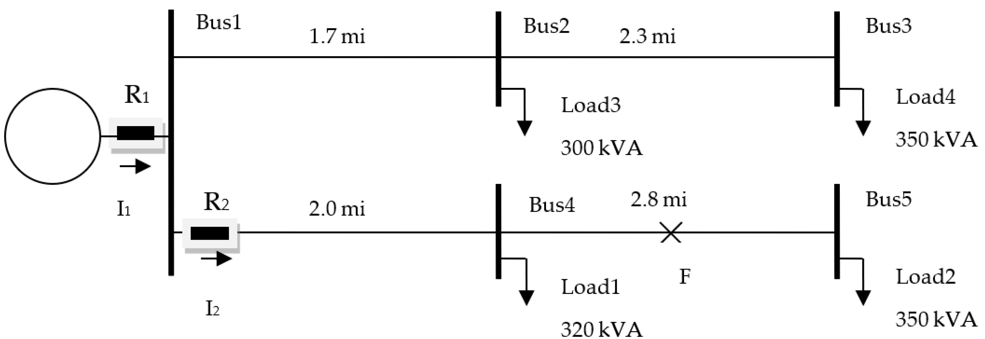
2.1. Five-Bus System
2.2. RTDS Model
- [0.3465 + j1.0179 0.1560 + j0.5017 0.1580 + j0.4236
- 0.1560 + j0.5017 0.3375 + j1.0478 0.1535 + j0.3849
- 0.1580 + j0.4236 0.1535 + j0.3849 0.3414 + j1.0348].
3. SEL-351 Relay Configuration
4. Relay Schemes
4.1. Instantaneous Overcurrent Scheme
4.2. Definite Time Overcurrent Scheme
4.3. Inverse Definite Minimum Time (IDMT) Overcurrent Scheme
- Step 1—When setting up coordination, start with the device that will be closest to the fault within the zone of protection, i.e., relay R2 in this study.
- Step 2—Select the appropriate relay settings for both relays as shown in Table 1.
- Step 3—Calculate the operating time and time dial setting (51PTD) for both relay R1 and R2. Initially, the operating time of R2 will be calculated. The equation used to calculate the operating time is selected as per the IDMT curve (51PC) chosen for the relay. Since curve U3 has been selected for R2, the following formula (given in SEL-351’s instruction manual) will be used to calculate the operating time:where, M is a multiple of the pickup current setting, and is the time dial setting of R2. In this experiment, for R2, the value of M is 29.32 (14.66 / 0.5, where 0.5 is the pickup current setting of R2) (see Section 2.2), and the value of 51PTD is 1. Hence, the operating time of relay R2 will be as follows:
- Step 4—To calculate the operating time of R1, determine the operating time of R2 and a Coordination Interval (CI) between both relays. CI is required to ensure proper coordination with upstream devices (R1 in this case). It ensures that R2 has enough time to operate before R1 begins to operate.
- Step 5—Using the parameters in step 3 and 4, calculate 51PTD of R1 as follows:where M is 14.75 (14.75/1, where 1 is the pickup current setting of R1), as calculated in Section 2.2.
5. Interfacing Relays with RTDS
5.1. GTAO Card
5.1.1. GTAO Scaling When Using Relay’s Low-Level Interface
Calculating Required Voltage Output from GTAO Card for Input Current Parameters
- Step 1—Calculate the secondary side value of the fault current. In this case, the CTR is 120 (i.e., 120:1). Therefore,
- Step 2—To calculate the required output voltage from the GTAO card, divide the secondary current by the scaling factor of the relay. In our case, the scale was 50, as shown in Table 2. Therefore,
Calculating Required Output from GTAO Card for Input Voltage Parameters
- Step 1—Calculate the value on the secondary side of the relay by dividing fault current by PTR. In our case, the PTR was 60 (i.e., 60:1). Therefore,
- Step 2—To calculate the required output voltage from the GTAO card, divide the secondary voltage by the scaling factor of the relay. In this case, the scale factor was 102, as shown in Table 2. Therefore,
5.1.2. GTAO Scaling When Using CMS 356
5.2. Obtaining Readings on the Relay Front Panel
5.3. GTFPI Card
5.4. Applying Faults to the System
5.5. Circuit Breaker Logic
6. Results
6.1. Pre-Fault Period
6.2. Fault Period (Instantaneous and Definite Time Scheme)
6.3. Post-Fault Period
6.4. Coordination between R1 and R2 (IDMT Scheme)
- Case 1—When R2 operates
- Case 2—When R1 operates
6.5. Relay Events
7. Conclusions
Author Contributions
Funding
Data Availability Statement
Acknowledgments
Conflicts of Interest
References
- Anderson, D.; Zhao, C.; Hauser, C.H.; Venkatasubramanian, V.; Bakken, D.E.; Bose, A. A Virtual Smart Grid. IEEE Power & Energy Magazine. February 2012, pp. 49–57. Available online: https://magazine.ieee-pes.org/january-february-2012/a-virtual-smart-grid/ (accessed on 23 October 2022).
- Nutaro, J. Designing power system simulators for the smart grid: Combining controls, communications, and electro-mechanical dynamics. In Proceedings of the IEEE Power and Energy Society General Meeting, Detroit, MI, USA, 24–28 July 2011. [Google Scholar] [CrossRef]
- McLaren, P.; Nayak, O.; Langston, J.; Steurer, M.; Sloderbeck, M.; Meeker, R.; Lin, X.; Yu, M.; Forsyth, P. Testing the ‘smarts’ in the smart T & D grid. In Proceedings of the IEEE/PES Power Systems Conference and Exposition (PSCE), Phoenix, AZ, USA, 20–23 March 2011; pp. 1–8. [Google Scholar] [CrossRef]
- Podmore, R.; Robinson, M.R. The role of simulators for smart grid development. IEEE Trans. Smart Grid 2010, 1, 205–212. [Google Scholar] [CrossRef]
- Montano, F.; Ould-Bachir, T.; David, J.P. An Evaluation of a High-Level Synthesis Approach to the FPGA-Based Submicrosecond Real-Time Simulation of Power Converters. IEEE Trans. Ind. Electron. 2018, 65, 636–644. [Google Scholar] [CrossRef]
- Chen, Y.; Dinavahi, V. Hardware emulation building blocks for real-time simulation of large-scale power grids. IEEE Trans. Ind. Inform. 2014, 10, 373–381. [Google Scholar] [CrossRef]
- Adegbohun, F.R.; Lee, K.Y. Real-time modeling, simulation and analysis of a grid connected PV system with hardware-in-loop protection. In Proceedings of the North American Power Symposium (NAPS), Morgantown, WV, USA, 17–19 September 2017. [Google Scholar] [CrossRef]
- Fan, W.; Liao, Y. Fault Location for Distribution Systems with Distributed Generations without Using Source Impedances. In Proceedings of the 51st North American Power Symposium (NAPS), Wichita, KS, USA, 13–15 October 2019. [Google Scholar] [CrossRef]
- Asbery, C.; Liao, Y. Fault Identification on Electrical Transmission Lines Using Artificial Neural Networks. Ph.D. Thesis, University of Kentucky, Lexington, KT, USA, 2022; pp. 13–14. [Google Scholar]
- Fan, W.; Liao, Y.; Kang, N. Optimal fault location for power distribution systems with distributed generations using synchronized measure-ments. Int. J. Emerg. Electr. Power Syst. 2020, 21, 20200093. [Google Scholar]
- Kuffel, R.; Forsyth, P.; Peters, C. The Role and Importance of Real Time Digital Simulation in the Development and Testing of Power System Control and Protection Equipment. IFAC-PapersOnLine 2016, 49, 178–182. [Google Scholar] [CrossRef]
- Tatcho, P.; Zhou, Y.; Li, H.; Liu, L. A real time digital test bed for a smart grid using RTDS. In Proceedings of the 2nd International Symposium on Power Electronics for Distributed Generation Systems (PEDG 2010), Hefei, China, 16–18 June 2010; pp. 658–661. [Google Scholar] [CrossRef]
- Marttila, R.J.; Dick, E.P.; Fischer, D.; Mulkins, C.S. Closed-loop testing with the real-time digital power system simulator. Electr. Power Syst. Res. 1996, 36, 181–190. [Google Scholar] [CrossRef]
- Mishra, P.; Pradhan, A.K.; Bajpai, P. Adaptive Relay Setting for Protection of Distribution System with Solar PV. In Proceedings of the 20th National Power Systems Conference (NPSC 2018), Tiruchirappalli, India, 14–16 December 2018; Volume 2, pp. 1–5. [Google Scholar] [CrossRef]
- Afshar, M.; Majidi, M.; Gashteroodkhani, O.A.; Amoli, M.E. Analyzing Performance of Relays for High Impedance Fault (HIF) Detection Using Hardware-In-The-Loop (HIL) Platform. Electr. Power Syst. Res. 2022, 209, 108027. [Google Scholar] [CrossRef]
- Chen, Y.; Wen, M.; Wang, Z.; Yin, X.; Peng, J.; Zhang, R. An improved numerical distance relay based on CCVT transient characteristic matching. Int. J. Electr. Power Energy Syst. 2020, 122, 106146. [Google Scholar] [CrossRef]
- Cho, Y.S.; Lee, C.K.; Jang, G.; Kim, T.K. Design and implementation of a real-time training environment for protective relay. Int. J. Electr. Power Energy Syst. 2010, 32, 194–209. [Google Scholar] [CrossRef]
- So, K.H.; Heo, J.Y.; Kim, C.H.; Aggarwal, R.K.; Kim, J.C.; Jang, G.S. An implementation of current differential relay and directional comparison relay using EMTP MODELS. Int. J. Electr. Power Energy Syst. 2006, 28, 261–272. [Google Scholar] [CrossRef]
- Dias, O.; Tavares, M.C.; Magrin, F. Hardware implementation and performance evaluation of the fast adaptive single-phase auto reclosing algorithm. Electr. Power Syst. Res. 2019, 168, 169–183. [Google Scholar] [CrossRef]
- Ledwaba, T.; Senyane, K.; Van Coller, J. Hardware-In-loop testing of a differential relay used to Protect single/double circuit transmission lines. In Proceedings of the Southern African Universities Power Engineering Conference/Robotics and Mechatronics/Pattern Recognition Association of South Africa (SAUPEC/RobMech/PRASA 2019), Bloemfontein, South Africa, 28–30 January 2019; pp. 347–352. [Google Scholar] [CrossRef]
- Naveen, P.; Jena, P. Directional Overcurrent Relays Coordination Scheme for Protection of Microgrid. In Proceedings of the IEEE First International Conference on Smart Technologies for Power, Energy and Control (STPEC 2020), Nagpur, India, 25–26 September 2020. [Google Scholar] [CrossRef]
- Singh, M.; Telukunta, V.; Srivani, S.G. Enhanced real time coordination of distance and user defined over current relays. Int. J. Electr. Power Energy Syst. 2018, 98, 430–441. [Google Scholar] [CrossRef]
- Langston, J.; Steurer, M.; Schoder, K.; Borraccini, J.; Dalessandro, D.; Rumney, T.; Fikse, T. Power hardware-in-The-loop simulation testing of a flywheel energy storage system for shipboard applications. In Proceedings of the IEEE Electric Ship Technologies Symposium (ESTS), Arlington, VA, USA, 14–17 August 2017; pp. 305–311. [Google Scholar] [CrossRef]
- Stifter, M.; Cordova, J.; Kazmi, J.; Arghandeh, R. Real-time simulation and hardware-in-the-loop testbed for distribution synchrophasor applications. Energies 2018, 11, 876. [Google Scholar] [CrossRef] [Green Version]
- Sidwall, K.; Forsyth, P. A Review of Recent Best Practices in the Development of Real-Time Power System Simulators from a Simulator Manufacturer’s Perspective. Energies 2022, 15, 1111. [Google Scholar] [CrossRef]


| Parameters | Relay R1 | Relay R2 |
|---|---|---|
| Pickup current setting (51PP) | 1 | 0.5 |
| IDMT curve (51PC) | U3 | U3 |
| Input Channels (Relay Rear Panel) | Input Channel Nominal Rating | Input Value | Corresponding J1 Output Value | Scale Factor (Input/Output) (A/V or V/V) |
|---|---|---|---|---|
| IA, IB, IC, IN | 1 A | 1 A | 100 mV | 10 |
| IA, IB, IC, IN | 5 A | 5 A | 100 mV | 50 |
| IN | 0.2 A | 0.2 A | 114.1 mV | 1.753 |
| IN | 0.05 A | 0.05 A | 50 mV | 1 |
| VA, VB, VC, VS | 150 V | 67 VLN | 1313.7 mV | 51 |
| VA, VB, VC, VS | 300 V | 134 VLN | 1313.7 mV | 102 |
| Power (+, −) | 48/125 Vdc or 125/120 Vdc | 125 Vdc | 1.25 Vdc | 100 |
| Parameter | Magnitude (RMS) | CTR | PTR | Relay Scale | GTAO Output | GTAO Scale |
|---|---|---|---|---|---|---|
| Current | 30 A | 120 | - | 50 | 0.67 V | 30 |
| Voltage | 7133 V | - | 60 | 102 | 1.63 V | 30.6 |
| Binary Value | Fault Type | Decimal |
|---|---|---|
| 001 | A-G | 1 |
| 010 | B-G | 2 |
| 100 | C-G | 4 |
| 110 | AB-G | 6 |
| 011 | BC-G | 3 |
| 101 | AC-G | 5 |
| 111 | ABC-G | 7 |
Disclaimer/Publisher’s Note: The statements, opinions and data contained in all publications are solely those of the individual author(s) and contributor(s) and not of MDPI and/or the editor(s). MDPI and/or the editor(s) disclaim responsibility for any injury to people or property resulting from any ideas, methods, instructions or products referred to in the content. |
© 2023 by the authors. Licensee MDPI, Basel, Switzerland. This article is an open access article distributed under the terms and conditions of the Creative Commons Attribution (CC BY) license (https://creativecommons.org/licenses/by/4.0/).
Share and Cite
Yadav, G.; Liao, Y.; Burfield, A.D. Hardware-in-the-Loop Testing for Protective Relays Using Real Time Digital Simulator (RTDS). Energies 2023, 16, 1039. https://doi.org/10.3390/en16031039
Yadav G, Liao Y, Burfield AD. Hardware-in-the-Loop Testing for Protective Relays Using Real Time Digital Simulator (RTDS). Energies. 2023; 16(3):1039. https://doi.org/10.3390/en16031039
Chicago/Turabian StyleYadav, Gaurav, Yuan Liao, and Austin D. Burfield. 2023. "Hardware-in-the-Loop Testing for Protective Relays Using Real Time Digital Simulator (RTDS)" Energies 16, no. 3: 1039. https://doi.org/10.3390/en16031039