Research on Magnetic Field and Force Characteristics of a Novel Four-Quadrant Lorentz Force Motor

Abstract

The 6-DOF vibration isolation platform (VIP) is used to isolate vibration in the processing and manufacturing of semiconductor chips, especially electric vehicle chips. The 6-DOF VIP has the characteristics of high position accuracy, fast dynamic response, and short motion travel. In this paper, a novel four-quadrant Lorentz force motor (FQLFM) applied on the 6-DOF VIP is proposed. The structure of this LFM has a high force density, low force fluctuation, and low coupling force. First, the basic structure and operating principle of the proposed FQLFM are presented. Secondly, the expressions of the magnetic field and electromagnetic force are obtained based on an equivalent current model and the permanent magnet mirror-image method (PMMIM). Thirdly, the magnetic field and electromagnetic force characteristics of the proposed FQLFM and an LFM with a traditional bilateral structure are analyzed and compared. The relationship between the force and displacement of the FQLFM is investigated. Moreover, the PMMIM is verified by a 3D finite element analysis (FEA). Finally, the experimental platform for a force test is built and the above results are validated by an experiment.

1. Introduction

With the increasingly stringent requirements for working environments in the processing and manufacturing of semiconductor chips, higher performance requirements have been put forward for the vibration control system, especially that applied on electric vehicle chips [1]. The 6-DOF magnetic suspension vibration isolation platform (VIP) uses electromagnetic force to isolate the isolated object from the vibration source [2,3]. A magnetic suspension VIP has the advantages of no mechanical contact, no friction, and compatibility with the vacuum environment, which is very suitable for the processing and manufacturing of electric vehicle chips.

The Lorentz force motor (LFM) is the key component of the 6-DOF VIP. The LFM is a kind of micro motor, which has lots of advantages, such as a simple structure, fast dynamic response, no cogging torque, and high linearity [4,5]. A 6-DOF VIP can be a combination of multi-unit LFMs with magnetic levitation gravity compensators and displacement sensors. In contrast to the LFM, which has a single degree of freedom, the LFM on the 6-DOF VIP needs to provide sufficient driving force. On this basis, the LFM on the VIP also needs to have a smaller volume, smaller force fluctuation, and smaller coupling force to achieve high-precision positioning [6,7]. In this paper, a novel LFM that is suitable for the 6-DOF VIP system is proposed, which is called a four-quadrant Lorentz force motor (FQLFM).

2. Basic Structure and Operating Principle

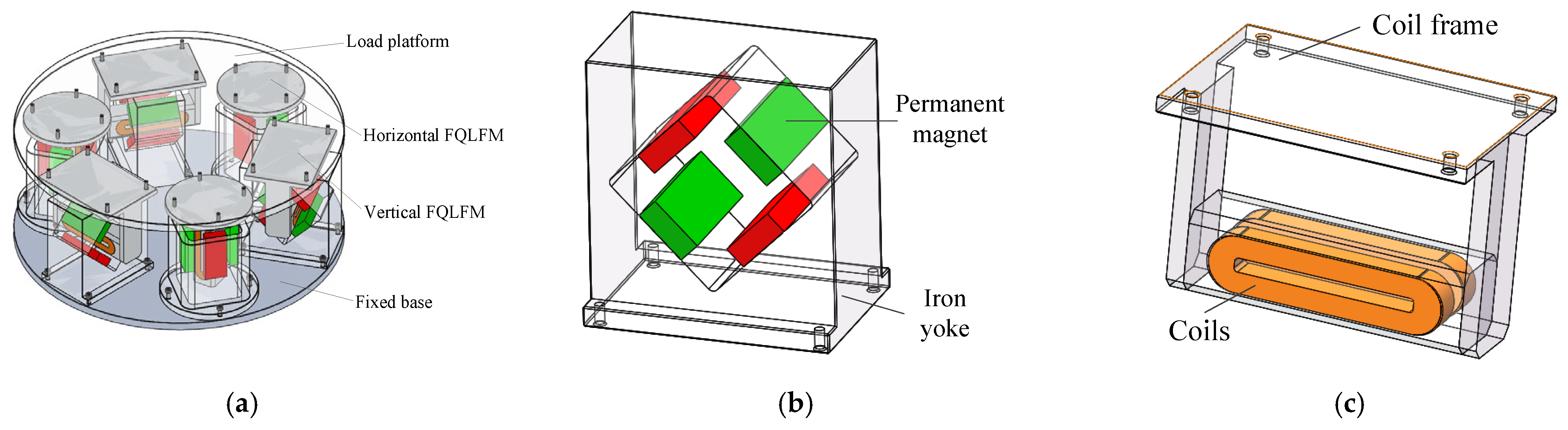
2.1. Basic Structure of FQLFM

Figure 1 shows the basic structure of the 6-DOF VIP and FQLFM. The 6-DOF VIP includes three horizontal FQLFMs and three vertical FQLFMs, as shown in Figure 1a. It consists of a load platform, a fixed base, limit devices, accelerometers, displacement sensors, and magnetic levitation gravity compensators. Generally, the 6-DOF VIP is fixed on a marble platform with a foundation.

Figure 1b,c shows that the FQLFM is composed of two parts, the stator and mover. The stator consists of four permanent magnets (PMs) distributed in four quadrants and an iron yoke out of the PMs, which is placed on a fixed base. The mover consists of two multi-turn racetrack-type coils and a coil frame, which is installed under the load platform.

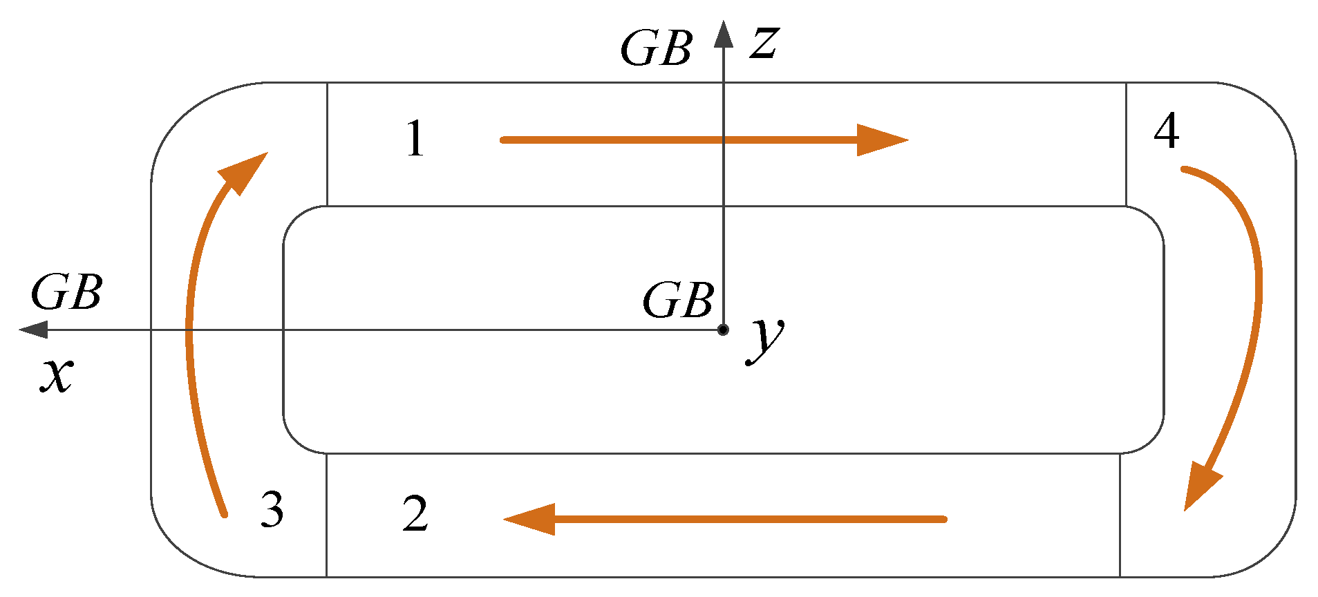
2.2. Operating Principle of FQLFM

The FQLFM has the same operating principle as a traditional LFM. When the energized conductor is in a constant magnetic field, the coils’ conductor will generate a Lorentz force. In order to change the size or direction of the Lorentz force, the current in the coils’ conductor should be adjusted [8,9]. A novel FQLFM is proposed in this paper which has the advantages of high force linearity, low force fluctuation, and low coupling force for improving the motion performance of the 6-DOF VIP. Due to the characteristics of the FQLFM, the difficulty in the control of the 6-DOF LFM can be reduced greatly [10,11].

The operating principle of the 6-DOF VIP composed of the FQLFM is as follows: the energized coils of the LFM generate driving force in a single direction, so that the load platform moves in this direction. It is necessary to install three horizontal FQLFMs around the load platform for controlling the load translation along the x, y axes and to rotate them around the z axis to realize motion with three degrees of freedom. In addition, three vertical FQLFMs are installed to control the load translation along the z axis and the rotation around the x, y axes for motion with three further degrees of freedom [12,13,14,15].

3. Mathematical Model

According to Ampere’s molecular current hypothesis, the magnetic field generated by the surface current is used to replace the one by the PM, and the PMMIM is adopted instead of the effect of the iron yoke. So the specific calculation process for the magnetic field and electromagnetic force of the FQLFM is as follows:

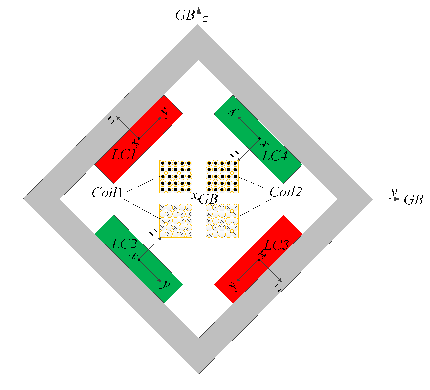
3.1. Establishment of Coordinate System

Figure 2 shows the coordinate system of the FQLFM, including a global coordinate system and four local coordinate systems. The geometric center point of the stator iron yoke is defined as the origin point of the global coordinate system (GB), and the geometric center points of four PMs are the origin points of four local coordinate systems (LCx), which are called LC1, LC2, LC3, LC4, respectively [16].

Figure 3 shows eight 3D coordinates points to describe the basic structural parameters of one PM. The magnetization direction of one PM is the positive z-axis in LCx.

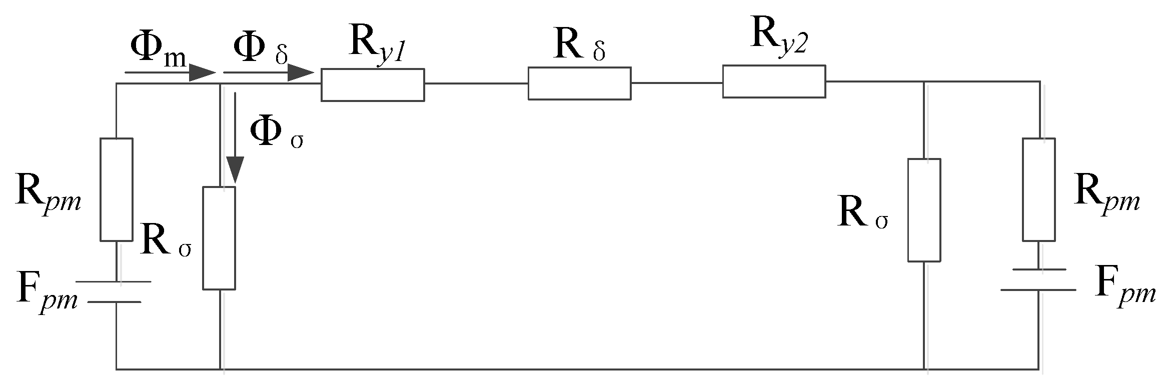
3.2. Magnetic Field of FQLFM

As is known, the magnetic field produced by one single PM is equivalent to a set of current sources; the equivalent current density of one PM can be expressed as follows [17]:

$$j_m=M\times n$$

(1)

where j_m is the equivalent surface current density, M is the coercivity of PM, and n is the normal unit vector.

The magnetic flux density generated by equivalent current is expressed as:

$$B(r)=\frac{{\mu }_0}{4\pi }{\displaystyle {\int }_S{j}_m\times \frac{\left(r-r^{\prime }\right)}{{\left|r-r^{\prime }\right|}^3}ds}$$

(2)

where μ₀ is the vacuum permeability, r is the position vector of a point in space, and r’ is the position vector of a point in one PM.

In LCx, the magnetic flux density generated by one single PM is expressed as [18]:

$${}^{LCx}{B}_x(x,y,z)=\frac{{\mu }_{0}M}{4\pi }{\displaystyle \sum _{i=1}^2{\displaystyle \sum _{j=1}^2{\displaystyle \sum _{k=1}^2{\left(-1\right)}^{i+j+k+1}}}}\times \ln \left[G_1(x,y,z,x_i,y_j,z_k)\right]$$

(3)

$$G_1{=}^{LCx}y{-}^{LCx}{y}_j+\left[{\left({}^{LCx}x{-}^{LCx}{x}_i\right)}^2\right.{\left.+{\left({}^{LCx}y{-}^{LCx}{y}_j\right)}^2+{\left({}^{LCx}z{-}^{LCx}{z}_k\right)}^2\right]}^{\frac{1}{2}}$$

(4)

$${}^{LCx}{B}_y(x,y,z)=\frac{{\mu }_{0}M}{4\pi }{\displaystyle \sum _{i=1}^2{\displaystyle \sum _{j=1}^2{\displaystyle \sum _{k=1}^2{\left(-1\right)}^{i+j+k+1}}}}\times \ln \left[G_2(x,y,z,x_i,y_j,z_k)\right]$$

(5)

$$G_2{=}^{LCx}x{-}^{LCx}{x}_i+\left[{\left({}^{LCx}x{-}^{LCx}{x}_i\right)}^2\right.+{\left.{\left({}^{LCx}y{-}^{LCx}{y}_j\right)}^2+{\left({}^{LCx}z{-}^{LCx}{z}_k\right)}^2\right]}^{\frac{1}{2}}$$

(6)

$${}^{LCx}{B}_z(x,y,z)=\frac{{\mu }_{0}M}{4\pi }{\displaystyle \sum _{i=1}^2{\displaystyle \sum _{j=1}^2{\displaystyle \sum _{k=1}^2{\left(-1\right)}^{i+j+k+1}}}}\times {\tan }^{-1}\left[G_3(x,y,z,x_i,y_j,z_k)\right]$$

(7)

$$G_3={(}^{LCx}x{-}^{LCx}{x}_i){(}^{LCx}y{-}^{LCx}{y}_j){{(}^{LCx}z{-}^{LCx}{z}_k)}^{-1}\times \left[{\left({}^{LCx}x{-}^{LCx}{x}_i\right)}^2+{\left({}^{LCx}y{-}^{LCx}{y}_j\right)}^2\right.{\left.+{\left({}^{LCx}z{-}^{LCx}{z}_k\right)}^2\right]}^{{}^{-\frac{1}{2}}}$$

(8)

$${}^{LCx}B{(}^{LCx}x{,}^{LCx}y{,}^{LCx}z){=}^{LCx}{B}_x{}^{LCx}{e}_x{+}^{LCx}{B}_y{}^{LCx}{e}_y{+}^{LCx}{B}_z{}^{LCx}{e}_z$$

(9)

where ^LCxx, ^LCxy, and ^LCxz are the spatial position coordinates in LCx; ^LCxx₁, ^LCxx₂, ^LCxy₁, ^LCxy₂, ^LCxz₁, and ^LCxz₂ are the coordinates of one PM in LCx; and ^LCxe_x, ^LCxe_y, and ^LCxe_z are the unit vectors in LCx.

When the PMs are distributed among the iron yoke, the magnetic field will change and will not be freely distributed anymore. The magnetic field generated by the surface between the iron yoke and PM is different from that generated by a single PM, so it is difficult to calculate the magnetic field. In this paper, the mirror-image method is used to replace the effect of the iron yoke. The iron yoke in contact with the PM mirrors another PM in the same direction of the magnetization as the original PM, and the iron yoke adjacent to the PM is also mirrored as another PM in the opposite direction of the magnetization. Therefore, one PM with an iron yoke will be replaced by one original PM and five other mirror-image PMs as shown in Figure 4 [19].

Figure 4 shows the mirror-image diagram of one single PM. The PM in LCx is the original PM; the PMs in LC¹x, LC³x and LC⁴x are the mirror-image PMs of the original; and the PMs in LC²x and LC⁵x are the mirror-image PMs of the PM in LC¹x.

Finally, the permeability of the iron yoke is assumed to be negligible here, so the expression of the magnetic flux density generated by one single PM with an iron yoke is as follows:

$$\begin{array}{l}{}^{LCx}{B}_{\mathrm{total}}=B_{og}(x,y,z)+B_{im\mathrm{I}}(x,y,z)+B_{im\mathrm{II}}(x,y,z)\\ ={\displaystyle \sum _{i=0}^1{\displaystyle \sum _{j=-1,0,1}B\left({}^{LCx}x{,}^{LCx}y+j(w_y+\left|{}^{LCx}{y}_2{-}^{LCx}{y}_1\right|){,}^{LCx}z-i\left|{}^{LCx}{z}_2{-}^{LCx}{z}_1\right|\right)}}\end{array}$$

(10)

where B_og is the magnetic flux density of the original PM; B_imI and B_imII are the magnetic flux densities of the mirror-image PMs; and w_y is the distance between the original PM and mirror image PM in the horizontal direction.

Then, the magnetic field of one PM is transferred from LCx to GB. We set the spatial position coordinate matrix in GB as:

$${}^{GB}A={[}^{GB}x{,}^{GB}y{,}^{GB}z,1]$$

(11)

The spatial position coordinate matrix in LCx is as follows:

$${}^{LCx}A{=}^{LCx}{T}_{GB}{}^{LCx}{R}_{GB}{}^{{}^{GB}}A$$

(12)

where ^LCxT_GB is the translation matrix from GB to LCx, and ^LCxR_GB is the rotation matrix from GB to LCx.

$${}^{LCx}{T}_{GB}=\left[\begin{array}{cccc}1& 0& 0& {}^{GB}x{-}^{LCx}x\\ 0& 1& 0& {}^{GB}y{-}^{LCx}y\\ 0& 0& 1& {}^{GB}z{-}^{LCx}z\\ 0& 0& 0& 1\end{array}\right]$$

(13)

$$\begin{array}{l}{}^{LCx}{R}_{GB}=R_x{R}_y{R}_z=\left[\begin{array}{cccc}1& 0& 0& 0\\ 0& \cos {\theta }_x& \sin {\theta }_x& 0\\ 0& -\sin {\theta }_x& \cos {\theta }_x& 0\\ 0& 0& 0& 1\end{array}\right]\cdot \left[\begin{array}{cccc}\cos {\theta }_y& 0& -\sin {\theta }_y& 0\\ 0& 1& 0& 0\\ \sin {\theta }_y& 0& \cos {\theta }_y& 0\\ 0& 0& 0& 1\end{array}\right]\cdot \left[\begin{array}{cccc}\cos {\theta }_z& \sin {\theta }_z& 0& 0\\ -\sin {\theta }_z& \cos {\theta }_z& 0& 0\\ 0& 0& 1& 0\\ 0& 0& 0& 1\end{array}\right]\\ \end{array}$$

(14)

where ^GBx, ^GBy, ^GBz, ^LCxx, ^LCxy and ^LCxz, respectively, are the spatial positions in GB and LCx; and θ_x, θ_y and θ_z are the rotation angles of GB around the x, y, z axes of LCx.

Then, the magnetic flux density of one single PM in GB is as follows:

$${}^{GB}{B}_q{(}^{GB}x{,}^{GB}y{,}^{GB}z){=}^{GB}{R}_{LCx}{}^{LCx}{B}_{total}{(}^{LCx}\mathrm{A}[1:3])$$

(15)

The rotation matrix ^GBR_LCx is the inverse matrix of ^LCxR_GB, and it is expressed as:

$${}^{GB}{R}_{LCx}{=}^{LCx}{R}_{GB}{}^{-1}$$

(16)

Finally, the magnetic field generated by four PMs together in GB can be obtained as follows:

$${}^{GB}B{(}^{GB}x{,}^{GB}y{,}^{GB}z)={\displaystyle \sum _{q=1}^4{}^{GB}{B}_q{(}^{GB}x{,}^{GB}y{,}^{GB}z)}$$

(17)

3.3. Electromagnetic Force

In order to improve the accuracy of the electromagnetic force, the racetrack’s turning coils are divided into four parts; the currents of 1 and 2 are in the y direction and those of 3 and 4 are in the y, z directions as Figure 5 shows. The mover coils of the FQLFM include coil1 and coil2.

Using the Lorentz force formula, the expression of the electromagnetic force of the coils in each direction can be obtained as:

$$F_x={\displaystyle \sum _{p=1}^2\left({\displaystyle \underset{V_3+V_4}{\int }{J}_{zp}{\cdot }^{GB}{B}_y{(}^{GB}x{,}^{GB}y{,}^{GB}z)dv}\right)}$$

(18)

$$F_y={\displaystyle \sum _{p=1}^2\left({\displaystyle \underset{V_3+V_4}{\int }{J}_{zp}{\cdot }^{GB}{B}_x{(}^{GB}x{,}^{GB}y{,}^{GB}z)dv}+{\displaystyle \underset{V_1+V_2+V_3+V_4}{\int }{J}_{xp}{\cdot }^{GB}{B}_z{(}^{GB}x{,}^{GB}y{,}^{GB}z)dv}\right)}$$

(19)

$$F_z={\displaystyle \sum _{p=1}^2\left({\displaystyle \underset{V_1+V_2+V_3+V_4}{\int }{J}_{xp}{\cdot }^{GB}{B}_y{(}^{GB}x{,}^{GB}y{,}^{GB}z)dv}\right)}$$

(20)

$$F=F_x{\cdot }^{GB}{e}_x+F_y{\cdot }^{GB}{e}_y+F_z{\cdot }^{GB}{e}_z$$

(21)

where F_x, F_y and F_z are the electromagnetic force of the coils in the x, y, z directions; B_x, B_y, and B_z are the magnetic flux densities in the x, y, z directions; J_x and J_z are the current densities in the x, z directions; V₁ and V₂ are the volume of the coils’ straight-edge region; and V₃ and V₄ are the volume of the coils’ end region.

4. Finite Element Analysis

4.1. 3D Models of Two Kinds of LFM

Considering of the 6-DOF motion of a VIP, a 2D finite element analysis (FEA) is unable to accurately analyze the magnetic field distribution and electromagnetic force of the FQLFM [20]. Therefore, a 3D FEA is adopted in this paper. Moreover, the magnetic flux density, force fluctuation, and coupling force of the FQLFM are compared with those of the LFM of a traditional bilateral structure (LFMOTBS) by a 3D FEA.

Figure 6 shows a 3D model and the coordinate systems of the FQLFM and LFMOTBS. The direction of the electromagnetic thrust is the same, which is pointing to the z-axis, although the magnetic field direction is inconsistent.

Table 1. Basic structural parameters of two motors.

Parameter	FQLFM	LFMOTBS	Material
Width of PM	20 mm	20 mm	NdFeb N35
Thickness of PM	8 mm	8 mm
Length of PM	45 mm	45 mm
Width of coils	8 mm	7 mm	Copper
Thickness of coils	8 mm	7 mm
Length of coils	60 mm	60 mm
Turns of coils	64	50
Thickness of iron yoke	7 mm	7 mm	DT4
Min gap length	3 mm	3 mm	Air

shows the basic structural parameters of the FQLFM and LFMOTBS. The sizes of the PM and iron yoke with the two models are the same; only the turns of the coils are different. The turns of the FLMOTBS are less than those of the FQLFM.

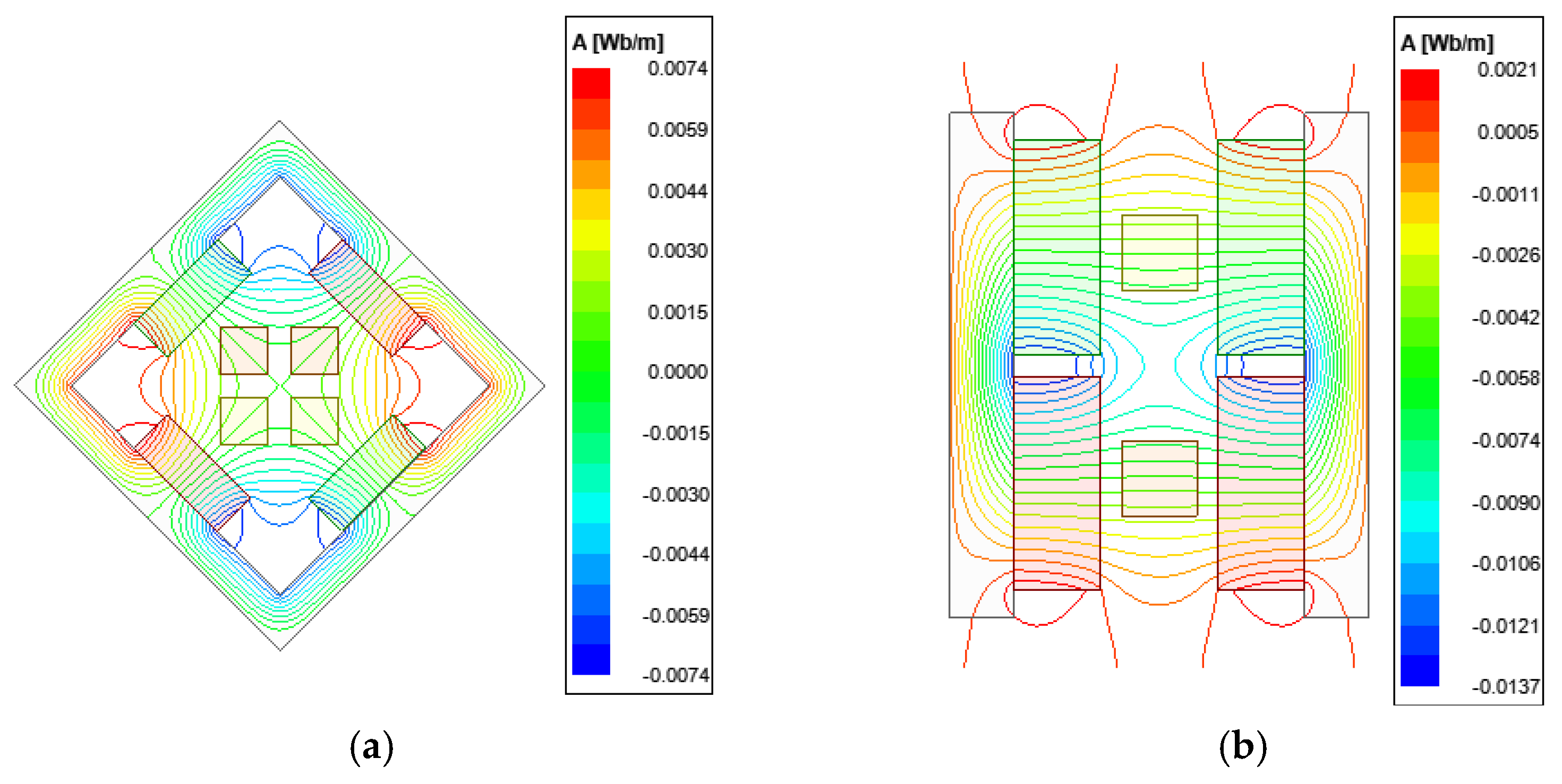
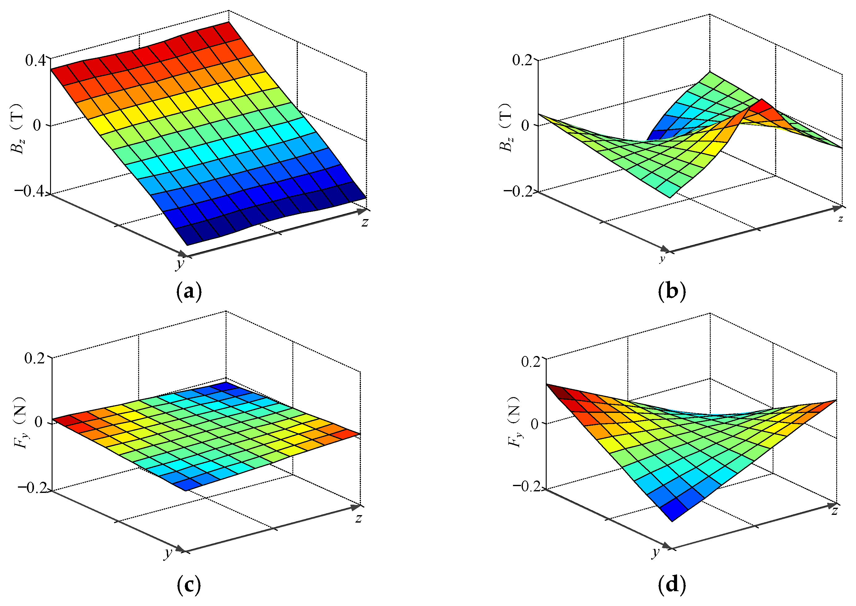
4.2. Magnetic Field and Force Compared between FQLFM and LFMOTBS

Figure 7 shows the magnetic field distribution of the FQLFM and LFMOTBS. The effective magnetic field of the FQLFM is generated by the interaction of the magnetic field with the adjacent PM. The one of the LFMOTBS is generated by the opposite PM. The air gap length of the FQLFM is obviously larger than that of the LFMOTBS.

When the range of the mover motion is ±1 mm (y) to ±1 mm (z) and the electromagnetic thrust (F_z) is about 10.62 N, the distribution cloud of the magnetic flux density in the y direction (B_y) and the electromagnetic thrust of the FQLFM and LFMOTBS are as shown below in Figure 8.

According to Figure 8, when the number, shape, and size of the PMs with two LFMs are the same, the LFMOTBS can produce the same electromagnetic thrust as the FQLFM with fewer coil turns. However, the magnetic flux density of the FQLFM along the z-axis is linearly changed and the one along the y-axis is the same as shown in Figure 8a. In contrast, the magnetic flux density of the LFMOTBS along the z-axis does not linearly change and is similar to a sine curve, the magnetic field along the y-axis is also no longer evenly distributed, and the center is weaker than that of the end as shown in Figure 8b.

Since the magnetic field of the FQLFM in the y direction is linear, the increased force at the upper part of the energized coils is equal to the reduced force at the bottom of the coils, so the electromagnetic thrust almost remains unchanged. However, the magnetic field of the FQLFM is also weakly distorted. The electromagnetic thrust fluctuation of the FQLFM is 0.15%, whereas that of the LFMOTBS is 1.16%. Therefore, the electromagnetic thrust with the FQLFM has lower force fluctuation than that of the LFMOTBS as shown in the comparison in Figure 8c,d.

The coupling force of the LFM also should be considered, in addition to the electromagnetic thrust fluctuation. In the 6-DOF VIP, the magnetic levitation gravity compensator is not constrained by a guide rail device, and the coupling force of the LFM in the non-driving direction will affect the magnetic levitation system, so the coupling force of the LFM needs to be considered.

Figure 9 shows the magnetic field distribution cloud in the z direction (B_z) and the coupling force in the y direction (F_y) between the FQLFM and LFMOTBS when the range of the mover’s motion is ±1 mm (y) to ±1 mm (z).

It can be seen from Figure 9a that the magnetic flux density distribution of the FQLFM is linear like Figure 8a. However, the magnetic flux density of the LFMOTBS is unevenly distributed as shown in Figure 9b. Then the coupling force of the FQLFM is within ±16 mN, whereas the coupling force of the LFMOTBS is about ±124 mN as shown in Figure 9c,d. Therefore, the FQLFM not only has lower electromagnetic thrust fluctuation, but also has lower coupling force, which is very suitable for the 6-DOF VIP.

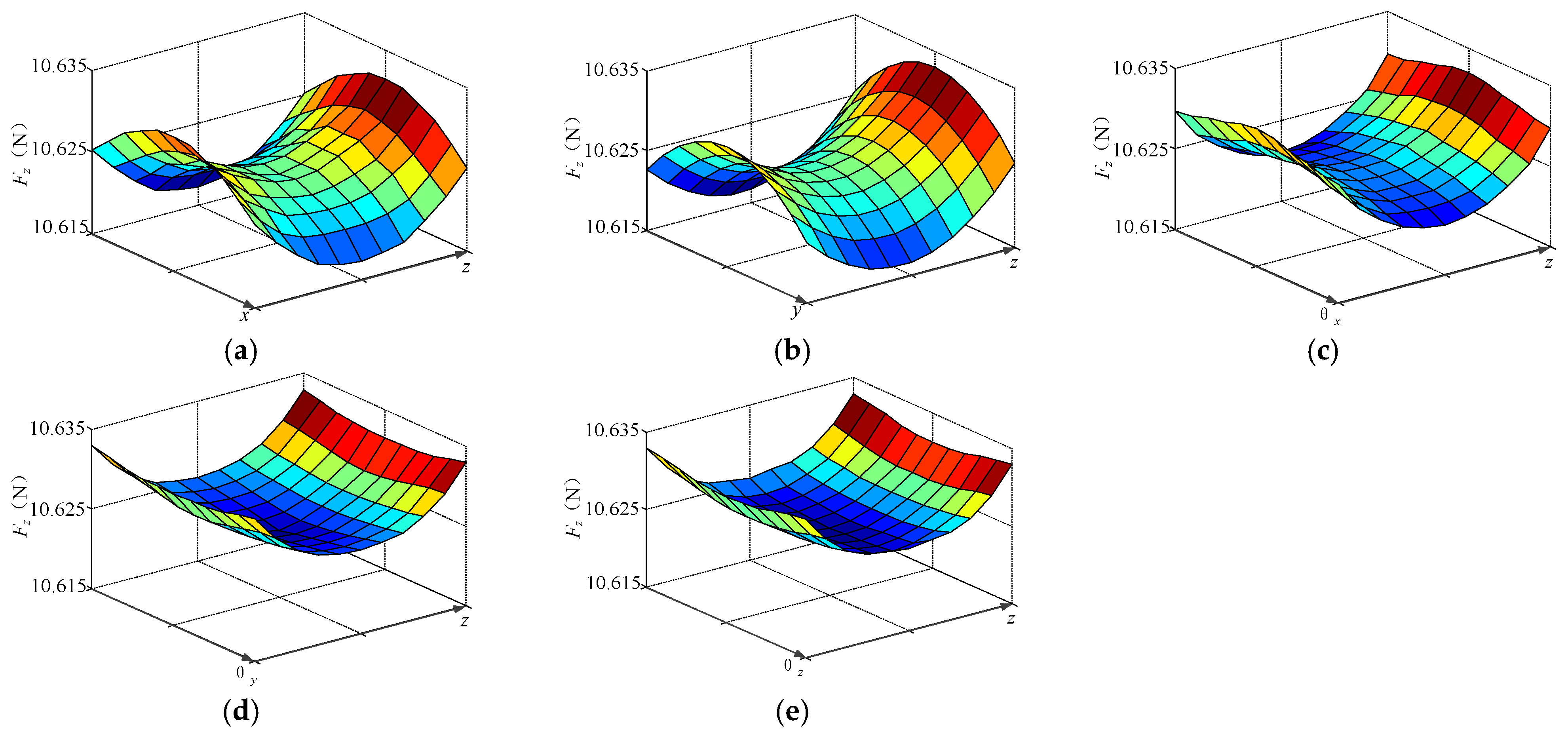
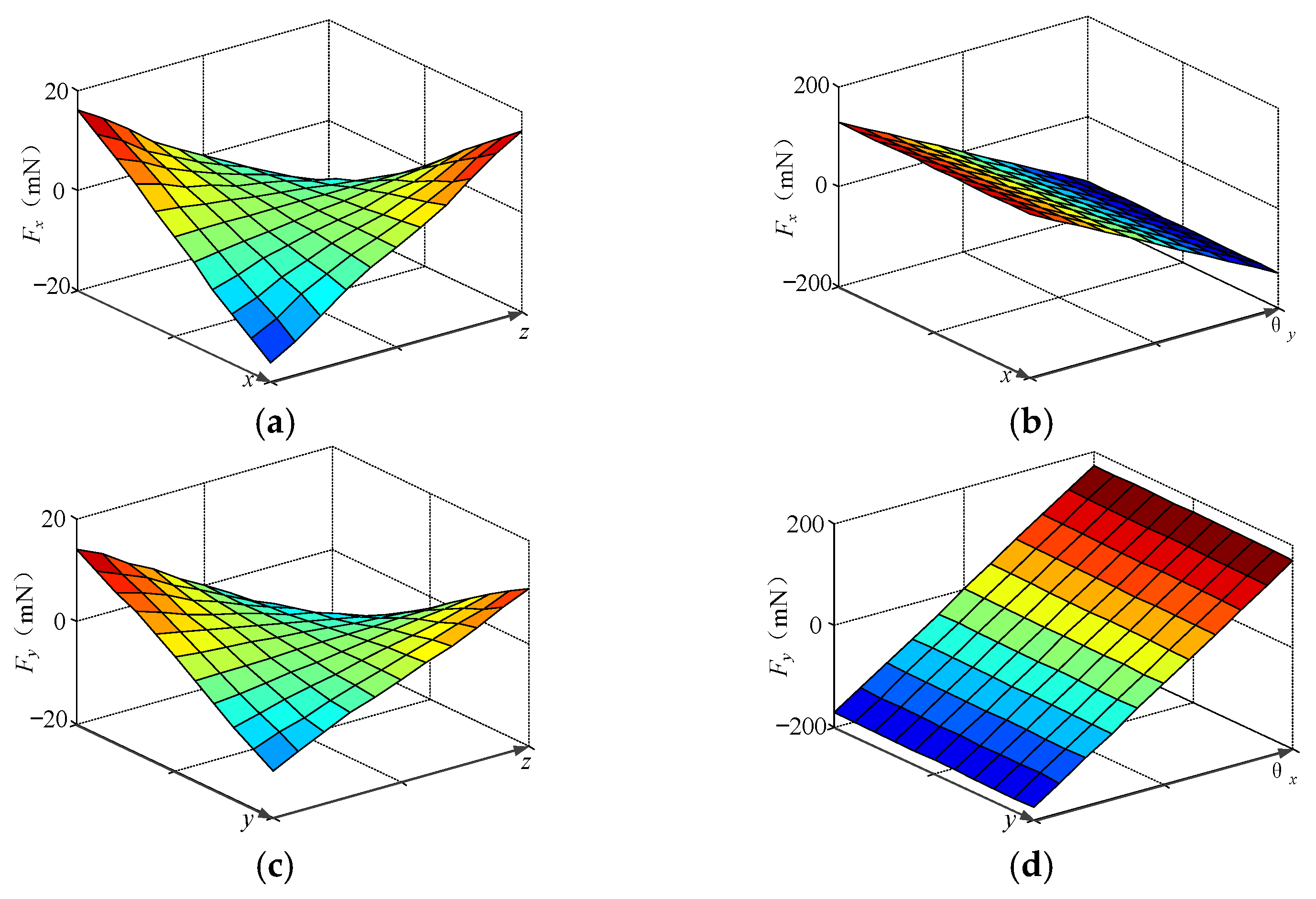
4.3. Force Characteristics of FQLFM

When the FQLFM is applied on the 6-DOF VIP, the electromagnetic thrust and coupling force caused in the y and z directions have been analyzed above and the ones in other directions and other angles also need to be analyzed.

The Figure 10 shows the distribution cloud of electromagnetic thrust when the relative position between the stator and mover is changed from −1 mm to 1 mm along the x, y, z axes, and the angle is changed from −1° to 1° around the x, y, z axes.

It can be seen from Figure 10 that the electromagnetic thrust is constant at 10.625 N throughout the whole stroke. The maximum thrust fluctuation of F_z caused by the 6-DOF is 0.16%. It proves that the FQLFM can effectively reduce the thrust fluctuation.

Figure 11 shows the variation curves of the coupling force in the x, y directions. Figure 11a,b shows that F_x is a linear increasing or decreasing translation along the x, z axes and F_x is still a linear decreasing rotation around the y axis. Figure 11c,d shows that F_y has the same rule translation along the y, z axes and rotation around the x axis. In this case, the negative effect of the coupling force can be eliminated by adding a compensation coefficient in the control system [21,22]. It should be mentioned that the size of the coupling force caused by other directions of motion is within 2 mN, so the effect is ignored.

4.4. Verification by FEA on PM Mirror-Image Method

In Section 3, the PM mirror-image method is used to derive the expression of magnetic flux density; now this method is verified by a 3D FEA. A 3D model of the LFM using the permanent magnet mirror-image method (PMMIM) is established, and the magnetic field distribution is shown in Figure 12. Figure 12b shows that the magnetic field is enhanced by increasing the thickness and number of PMs compared with Figure 7a.

Figure 13 shows the comparison of the magnetic field distribution and electromagnetic thrust between the original FQLFM and the LFM of the PMMIM when the range of the mover motion is ±1 mm (y) to ±1 mm (z). Figure 13 shows that magnetic field distributions of the two models are the same, but the size of the original FQLFM is about 0.02 T less than the LFM of the PMMIM from Figure 13a,b. Moreover, the size of the electromagnetic thrust with the original FQLFM is 0.6 N less than the LFM of the PMMIM, and the size of the coupling force is almost the same as shown in Figure 13c,d.

The analysis above shows that the magnetic flux density and electromagnetic thrust calculated by the PMMIM are consistent with those of the original FQLFM, but the electromagnetic thrust error is about 5% due to ignoring the saturation of the iron yoke. Therefore, in order to obtain more accurate expressions of the magnetic flux density and electromagnetic force, the influence of the saturation coefficient of the iron yoke should be considered.

Equation (10) is changed into the expression below:

$$\begin{array}{l}{}^{LCx}{B}_{\mathrm{total}}=B_{og}(x,y,z)+B_{im\mathrm{I}}(x,y,z)+B_{im\mathrm{II}}(x,y,z)\\ ={\displaystyle \sum _{i=0}^1\left(\left(k_{\mu }^i\cdot B{(}^{LCx}x{,}^{LCx}y{,}^{LCx}z-i\left|{}^{LCx}{z}_2{-}^{LCx}{z}_1\right|)\right)+{\displaystyle \sum _{j=0}^1\left(k_{\mu }^{j+1}\cdot B{(}^{LCx}x{,}^{LCx}y+{\left(-1\right)}^i\cdot (w_y+\left|{}^{LCx}{y}_2{-}^{LCx}{y}_1\right|){,}^{LCx}z)\right)}\right)}\end{array}$$

(22)

where k_μ is the relative permeability of the iron yoke. The expression of k_μ is as follows:

$$k_{\mu }=({\mu }_{Fe}-{\mu }_0)/({\mu }_{Fe}+{\mu }_0)$$

(23)

where μ_Fe is the permeability of the iron yoke, and μ₀ is the permeability of air. μ_Fe can be calculated by the equivalent magnetic circuit method.

Figure 14 shows a partial equivalent magnetic field diagram of the FQLFM, including the distribution of the main magnetic field and the leakage magnetic field.

In view of the periodic variation in the magnetic field distribution of the FQLFM, the equivalent magnetic circuit is established by a quarter model as shown in Figure 14. The main magnetic circuit starts from one half of the PM, passes through the circular arc gap, reaches the other half of the PM, and closes with a partial horizontal iron yoke and vertical iron yoke. The magnetic leakage circuit is the closure magnetic field of PM by itself and the closure magnetic field of the adjacent PM without passing through the iron yoke. Figure 15 shows the simplified equivalent magnetic circuit of the FQLFM, which is used to calculate the permeability of iron yoke μ_Fe.

According to Kirchhoff’s first and second laws, the following equations are established.

$${\Phi }_m={\Phi }_{\delta }+{\Phi }_{\sigma }$$

(24)

$$2\cdot M{h}_{pm}-2\cdot R_{pm}\cdot {\Phi }_m=(R_{y1}+R_{\delta }+R_{y2})\cdot {\Phi }_{\delta }$$

(25)

where Φ_m is the total magnetic flux, Φ_δ is the main magnetic flux, Φ_σ is the leakage magnetic flux, h_pm is the PM thickness, R_pm is the PM reluctance, R_y1 is the horizontal iron yoke reluctance, R_y2 is the vertical iron yoke reluctance, and R_δ is the air gap reluctance.

The magnetic leakage coefficient is defined as:

$$\sigma =\frac{{\Phi }_m}{{\Phi }_{\delta }}$$

(26)

Equation (25) can be combined with Equation (26) for the expression of the main magnetic flux, and the expression of reluctance is as follows.

$${\Phi }_{\delta }=\frac{2M{h}_{pm}}{2R_y{}_1+R_{\delta }+2\sigma R_{pm}}$$

(27)

$$R_y{}_1=R_y{}_2=\frac{w_{{}_{y1}}}{{\mu }_{Fe}{h}_y{l}_{ef}}=\frac{2w_y-w_{pm}-2h_y}{4\cdot {\mu }_{Fe}{h}_y{l}_{ef}}$$

(28)

$$R_{\delta }=\frac{h_{\delta }}{{\mu }_0{l}_{ef}{w}_{pm}/2}$$

(29)

$$R_{pm}=\frac{h_{pm}}{{\mu }_{pm}{l}_{ef}{w}_{pm}/2}=\frac{2h_{pm}}{{\mu }_{pm}{l}_{ef}{w}_{pm}}$$

(30)

where w_y is the iron yoke width, w_pm is the PM width, h_y is the iron yoke thickness, l_ef is the axis length of the FQLFM, μ_PM is the permeability of the PM, and h_δ is the average length of the air gap, which is calculated as Figure 16 shows.

$$\theta =\arctan [(h_{pm}+h_y/2)/w_{y1}]=\arctan \frac{4h_{pm}+2h_y}{2w_y-w_{pm}-2h_y}$$

(31)

$$h_{\delta }=\frac{(45-\theta )\pi }{90}\cdot (h_{pm}+h_y/2)/\sin \theta$$

(32)

The relationship between the magnetic flux density of iron yoke B_Fe and the magnetic field intensity of iron yoke H_Fe is as follows:

$$B_{Fe}={\mu }_{Fe}{H}_{Fe}$$

(33)

Equation (34) gives the relationship between B_Fe and H_Fe via (27)–(33).

$$B_{Fe}=-\frac{H_{Fe}(2w_y-w_{pm}-2h_y)}{2h_y{l}_{ef}(R_{\delta }+2\sigma R_{pm})}+\frac{2M{h}_{pm}}{h_y{l}_{ef}(R_{\delta }+2\sigma R_{pm})}$$

(34)

The permeability of the iron yoke can be obtained by combing Equation (34) with the magnetization curve of the magnetic material. As shown in Figure 17, the abscissa of the intersection between the two curves is the solution of the magnetic permeability of the iron yoke while working.

5. Experimental Verification

5.1. Experimental Setup

According to the analytical calculation and simulation results, a prototype of the FQLFM is manufactured. The specific structure parameters are shown in Table 1.

Figure 18 shows the electromagnetic thrust characteristic test platform of the FQLFM, which consists of a 3-DOF manual position adjuster, a three-axis force sensor, a high-precision multimeter, DC power supplies, and a support besides the stator and the mover of the FQLFM. The mover part of the FQLFM is fixed on the support, which is fixed on the marble platform. The stator of the FQLFM is connected with the 3-DOF manual position adjuster through the three-axis force sensor, and then the 3-DOF manual position adjuster also is fixed to the marble platform. The relative position relationship between the stator and mover of the FQLFM can be changed by adjusting the position of the 3-DOF manual position adjuster [23]. Although the relative position between the stator and mover is the opposite of those of the 6-DOF VIP, the electromagnetic thrust test result is the same based on Newton’s third law.

5.2. Force Characteristic Comparison

Figure 19 below shows the result between the electromagnetic thrust and coil current of the FQLFM, including three methods: an analytical calculation, 3D FEA, and experimental test.

Figure 19 shows that the electromagnetic thrust of the FQLFM linearly increased with the increase of coil current, so the FQLFM has good electromagnetic thrust linearity, and the thrust constant is about 2.125 N/A. In addition, the experimental results are in good agreement with the analytic calculation and 3D FEA results. When the coil current is 5.00 A, the analytical value of the thrust, the 3D FEA value, and the experimental value are 10.732 N, 10.626 N, and 10.402 N, respectively, and the maximum error among them is about 3.1%.

Figure 20 shows a distribution cloud between the electromagnetic thrust and displacement of the FQLFM via an experimental test. The positioning accuracy of the 3-DOF manual position adjuster is ±2.5 μm and the accuracy of the three-axis force sensor is 0.002 N, which meets the requirements of the experimental test.

Figure 20 shows that the variation curves of the electromagnetic thrust via manual adjustment are displaced from −1 mm to 1 mm in the x, y, z directions of the 3-DOF manual position adjuster, respectively, when the coil current is kept at 5.00 A. It can be seen from Figure 20a that the maximum thrust fluctuation is about a 0.23% translation along the x, z axes. The maximum thrust fluctuation is about 0.21% along the y, z axes as shown in Figure 20b. In fact, the FQLFM moves repeatedly with a smaller stroke and less thrust fluctuation.

Figure 21 shows a comparison of the electromagnetic thrust values between the analytic calculation, 3D FEA, and experimental test when the coil current is 5.00 A and travel length is a −1 mm to 1 mm translation along the x, y and z axes. It can be seen that the experimental results are in good agreement with the analytical calculation and 3D FEA. The maximum error among these is within 3.5% over the whole travel length.

6. Conclusions

In this paper, a novel FQLFM that is suitable for the 6-DOF VIP system is proposed. The expressions of the magnetic field and electromagnetic force are obtained based on an equivalent current model and the PMMIM. Then it is concluded that the effect of the iron yoke saturation coefficient should be considered to obtain more accurate expressions of magnetic flux density and electromagnetic force. Then, it is proved that the FQLFM has lower electromagnetic thrust fluctuation and lower coupling force than the LFMOTBS within the range of travel by the 3D FEA, although the force density of the LFMOTBS is higher than that of the FQLFM. Lastly, the above results are validated by experiment, and the maximum thrust error among the analytic calculation, 3D FEA, and experimental test is 3.5%. Moreover, the maximum electromagnetic thrust fluctuation caused by translation along the x, y, and z axes is 0.23% at a travel length of ±1 mm × ±1 mm × ±1 mm.

References

1. Maurya, S.K.; Galvan, H.R.; Gautam, G.; Xu, X. Recent progress in transparent conductive materials for photovoltaics. Energies 2022, 15, 8698. [Google Scholar] [CrossRef]
2. Zhou, Y.; Kou, B.; Zhang, H.; Zhang, L.; Wang, L. Design, Analysis and Test of a Hyperbolic Magnetic Field Voice Coil Actuator for Magnetic Levitation Fine Positioning Stage. Energies 2019, 12, 1830. [Google Scholar] [CrossRef] [Green Version]
3. Tsuda, M.; Tamashiro, K.; Sasaki, S.; Yagai, T.; Hamajima, T.; Yamada, T.; Yasui, K. Vibration transmission characteristics against vertical vibration in magnetic levitation type HTS seismic/vibration isolation device. IEEE Trans. Appl. Supercond. 2009, 19, 2249–2252. [Google Scholar] [CrossRef]
4. Ainslie, M.D.; Weinstein, R.; Sawh, R.-P. An Explanation for Observed Flux Creep in Opposite Direction to Lorentz Force in Partially Magnetized Bulk Superconductors. IEEE Trans. Appl. Supercond. 2019, 29, 1004–1007. [Google Scholar] [CrossRef] [Green Version]
5. Chai, J.; Gui, X. Overview of structure optimization and application of voice coil motor. Trans. China Electrotech. Soc. 2021, 36, 1114–1125. [Google Scholar]
6. Li, Z.; Wu, K.; Guo, M.; Chen, Y.; Wen, Y.; Wang, L. Constrained model predictive control for six-DOF vibration isolator of the absolute marine gravimeter. In I2MTC; IEEE: Piscataway, NJ, USA, 2021; pp. 1–5. [Google Scholar]
7. Wei, Y.; Nguyen, V.H.; Kim, W.-J. A 3-D printed Halbach-cylinder motor with self-position sensing for precision motions. IEEE Trans. Mechatron. 2021, 27, 1489–1497. [Google Scholar] [CrossRef]
8. Shen, B.; Fu, L.; Geng, J.; Zhang, H.; Zhang, X.; Zhong, Z.; Huang, Z.; Coombs, T.A. Design of a superconducting magnet for Lorentz force electrical impedance tomography. IEEE Trans. Appl. Supercond. 2016, 26, 205–210. [Google Scholar] [CrossRef]
9. Meng, X.; Wang, C.; Song, L.; Nie, Q.; Wang, Z.; Jiang, H. Designing and controlling voice coil motor based on the mars gravity simulation. In Proceedings of the 2019 22nd International Conference on Electrical Machines and Systems(ICEMS), Harbin, China, 11–14 August 2019; pp. 1–4. [Google Scholar]
10. Liu, C.-S.; Lin, P.-D.; Lin, P.-H.; Ke, S.-S.; Chang, Y.-H.; Horng, J.-B. Design and characterization of miniature auto-focusing voice coil motor actuator for cell phone camera applications. IEEE Trans. Magn. 2009, 45, 155–159. [Google Scholar] [CrossRef]
11. Perez-Diaz, J.L.; Valiente-Blanco, I.; Diez-Jimenez, E.; Sanchez-Garcia-Casarrubios, J. Superconducting non-Contact device for precision positioning in cryogenic environments. IEEE/ASME Trans. Mechatron. 2014, 19, 598–605. [Google Scholar] [CrossRef]
12. Chen, Y.-D.; Fuh, C.-C.; Tung, P.-C. Application of voice coil motors in active dynamic vibration absorbers. IEEE Trans. Magn. 2005, 41, 1149–1154. [Google Scholar] [CrossRef]
13. Rovers, J.M.M.; Jansen, J.W.; Compter, J.C.; Lomonova, E.A. Analysis method of the dynamic force and torque distribution in the magnet array of a commutated magnetically levitated planar actuator. IEEE Trans. Ind. Electron. 2012, 59, 2157–2166. [Google Scholar] [CrossRef]
14. Zhang, H.; Kou, B.; Jin, Y.; Zhang, H. Modeling and analysis of a new cylindrical magnetic levitation gravity compensator with low stiffness for the 6-DOF fine stage. IEEE Trans. Ind. Electron. 2015, 62, 3629–3639. [Google Scholar] [CrossRef]
15. Xu, Q. Design and development of a compact flexure-based XY precision positioning system with centimeter range. IEEE Trans. Ind. Electron. 2014, 61, 893–903. [Google Scholar] [CrossRef]
16. Zhang, H.; Kou, B.; Zhang, H.; Jin, Y. A three-degree-of-freedom short-stroke Lorentz-force-driven planar motor using a Halbach permanent-magnet array with unequal thickness. IEEE Trans. Ind. Electron. 2015, 62, 3640–3650. [Google Scholar] [CrossRef]
17. Jansen, J.W.; van Lierop, C.M.M.; Lomonova, E.A.; Vandenput, A.J.A. Modeling of magnetically levitated planar actuators with moving magnets. IEEE Trans. Magn. 2007, 43, 15–25. [Google Scholar] [CrossRef] [Green Version]
18. Zhou, Y.; Kou, B.; Zhang, H.; Luo, J.; Gan, L. Force characteristic analysis of a linear magnetic bearing with rhombus magnet array for magnetic levitation positioning system. IEEE Trans. Magn. 2017, 53, 407–414. [Google Scholar] [CrossRef]
19. Zhu, H.; Teo, T.J.; Pang, C.K. Design and modeling of a six-degree-of-freedom magnetically levitated positioner using square coils and 2D Halbach arrays. IEEE Trans. Ind. Electron. 2017, 64, 440–450. [Google Scholar] [CrossRef]
20. Ravaud, R.; Lemarquand, G.; Lemarquand, V.; Depollier, C. Permanent magnet couplings: Field and torque three-dimensional expressions based on the Coulombian model. IEEE Trans. Magn. 2009, 45, 1950–1958. [Google Scholar] [CrossRef] [Green Version]
21. Xie, Y.; Tan, Y.; Dong, R. Nonlinear modeling and decoupling control of XY micro positioning stages with piezoelectric actuators. IEEE/ASME Trans. Mechatron. 2013, 18, 821–832. [Google Scholar] [CrossRef]
22. Zhang, Z.-P.; Menq, C.-H. Six-axis magnetic levitation and motion control. IEEE Trans. Robot. 2007, 23, 15–25. [Google Scholar] [CrossRef]
23. Chen, M.Y.; Lin, T.B.; Hung, S.K.; Fu, L.C. Design and experiment of a macro–micro planar maglev positioning system. IEEE Trans. Ind. Electron. 2012, 59, 4128–4139. [Google Scholar] [CrossRef]
Figure 1. Structure of 6-DOF VIP and FQLFM. (a) 3D model of 6-DOF VIP. (b) 3D model of FQLFM stator. (c) 3D model of FQLFM mover.
Energies 16 01091 g001
Figure 2. The coordinate system of FQLFM.
Energies 16 01091 g002
Figure 3. The coordinate relationship of one PM.
Energies 16 01091 g003
Figure 4. Mirror-image diagram of one PM.
Energies 16 01091 g004
Figure 5. Current distribution of turning coils.
Energies 16 01091 g005
Figure 6. 3D model of two motors. (a) Model of FQLFM. (b) Model of LFMOTBS.
Energies 16 01091 g006
Figure 7. Magnetic field distribution of two motors. (a) Magnetic field of FQLFM. (b) Magnetic field of LFMOTBS.
Energies 16 01091 g007
Figure 8. Magnetic flux density and electromagnetic thrust of two motors. (a) By of FQLFM. (b) By of LFMOTBS. (c) Fz of FQLFM. (d) Fz of LFMOTBS.
Energies 16 01091 g008
Figure 9. Magnetic flux density and coupling force of two motors. (a) Bz of FQLFM. (b) Bz of LFMOTBS. (c) Fy of FQLFM. (d) Fy of LFMOTBS.
Energies 16 01091 g009
Figure 10. Variation curves of electromagnetic thrust. (a) Fz and x, z. (b) Fz and y, z. (c) Fz and θx, z. (d) Fz and θy, z. (e) Fz and θz, z.
Energies 16 01091 g010
Figure 11. Coupling force in x, y directions. (a) Fx and x, z. (b) Fx and x, θy. (c) Fy and y, z. (d) Fy and y, θx.
Energies 16 01091 g011
Figure 12. 3D model and magnetic field distribution of PMMIM. (a) 3D Model. (b) Magnetic field distribution.
Energies 16 01091 g012
Figure 13. Comparison of magnetic flux density and electromagnetic thrust between original FQLFM and the LFM of the PMMIM. (a) By. (b) Bz. (c) Fz. (d) Fy.
Energies 16 01091 g013
Figure 14. Schematic diagram of equivalent magnetic field distribution.
Energies 16 01091 g014
Figure 15. Equivalent magnetic circuit of FQLFM.
Energies 16 01091 g015
Figure 16. Geometric relationship of air gap length calculation.
Energies 16 01091 g016
Figure 17. Calculation of relative permeability of iron yoke.
Energies 16 01091 g017
Figure 18. Experimental platform for electromagnetic thrust test.
Energies 16 01091 g018
Figure 19. Curve of electromagnetic thrust and coil current via three methods.
Energies 16 01091 g019
Figure 20. Variation curves of electromagnetic thrust by experimental test. (a) Fz and x, z. (b) Fz and y, z.
Energies 16 01091 g020
Figure 21. Comparison of electromagnetic thrust by three methods. (a) Fz and x, z. (b) Fz and y, z.
Energies 16 01091 g021