Abstract
With growing interest in sustainability and net-zero emissions, there has been a global trend to integrate wind power into energy grids. However, challenges such as the intermittency of wind energy remain, which leads to a significant need for accurate wind-power forecasting. Therefore, this study focuses on creating a wind-power generation-forecasting model using a machine-learning algorithm. In this study, we used the gradient-boosting machine (GBM) algorithm to build a wind-power forecasting model. Time-series data with a 15 min interval from Jeju’s wind farms were applied to the model as input data. The short-term forecasting model trained by the same month with the test set turns out to have the best performance, with an NMAE value of 5.15%. Furthermore, the forecasting results were applied to Jeju’s power system to carry out a grid-security analysis. The improved accuracy of wind-power forecasting and its impact on the security of electrical grids in this study potentially contributes to greater integration of wind energy.
1. Introduction
With rising concerns about climate change, values such as sustainability and net-zero emissions have recently emerged as objectives for governments and companies worldwide. To achieve this goal, various policies have been implemented to increase renewable energy. South Korea has followed this green trend by enforcing the “2050 Carbon Neutral Strategy” [1]. The government plans to achieve its objective of decarbonizing the economic structure through the energy transition. Domestic and international efforts have led to notable renewables. Following the IRENA report in 2022, there has been a continuous growth in renewable energy in terms of both capacity and production [2]. Among renewable-energy sources, wind energy had a 10% increase in capacity and a 12% increase in production in 2019 compared to 2018.
Jeju Island, which is the largest island in South Korea, has been transforming into a net-zero island by 2030 through the carbon-free island (CFI) initiative. One of its aims is to introduce additional renewable-energy equipment to fully meet its power demand by expanding the power capacity to 4085 MW and electricity production to 9268 GWh [3].
Among renewable resources, wind energy is evaluated as a major contributor to CO2 emission reduction. By 2050, wind energy has the potential to reduce 6.3 Gt of CO2 emissions, accounting for 27% of energy resources [4]. Another study showed that when applying various representative concentration pathway (RCP) scenarios, wind power is expected to mitigate climate change by 2100 by reducing temperatures from 0.3 to 0.8 °C [5].
Despite its outcomes and advantages, the intermittent characteristics of wind power remain an obstacle to the integration of wind power into electrical grids. The inability to match the electricity demand can lead to severe damage, such as blackouts. Statistics show that Jeju Island underwent severalpower failures during the summer of 2021, with the total number of households that experienced blackouts being 131,589 [6]. To solve this, significant improvements in the accuracy of wind-power forecasting should be achieved. Recently, artificial intelligence (AI) and machine learning have been highlighted as advanced weather-forecasting technologies. It is believed that the application of machine learning to wind-power forecasting could be advantageous, as it is adaptive to changes or new surroundings and its accuracy improves with experience.
Variable renewable energy (VRE) forecasting can generally be categorized into different timescales [7,8]. Accurate short-term forecasting of VRE allows stakeholders to benefit from better bidding in electricity markets, enhanced unit commitment, and improved operational planning [9]. In contrast, long-term forecasting can be used for future works such as planning extreme-weather preparation, appropriate distribution of balancing reserves, and so on. Therefore, this study intends to contribute to these advantages by implementing a wind-power forecasting model.
Numerous efforts have been made to improve the accuracy of predicting the outputs of wind power using advanced machine-learning methods. Chen and Folly developed artificial neural networks (ANNs) and adaptive neuro-fuzzy inference-system (ANFIS) models for short-term forecasting while building an autoregressive moving average (ARMA) model specialized in short-term forecasting [7]. Choi and Choi combined bidirectional long short-term memory (LSTM) and convolution neural network (CNN) methods, proposing a new hybrid model [10]. Biswas et al. improved the autoregressive integrated moving average (ARIMA) model by integrating it with algorithms like random forest (RF) or bagging classification and regression trees (BCART) [11]. Ahmadi et al. revealed that the gradient-boosting algorithm has the second-best forecasting accuracy, with a minimal gap from the lowest MAE for 1 hour time-interval data [12]. Singh et al. built wind-power forecasting models of the Yalova wind farm in Turkey using five different machine-learning algorithms: random forest, k-nearest neighbors (k-NN), gradient-boosting machines (GBM), decision tree, and extra tree regression [13]. Among the five regression models, GBM demonstrated the best performance with the lowest error rates. Bankefa et al. utilized the GBM method in the process of developing a hybrid model to determine variables that are closely related to wind power and found that wind speed has a huge impact on wind power [14]. Several past studies have primarily forecasted wind power using machine-learning algorithms such as ARIMA, LSTM, etc. Contrastively, the GBM algorithm has been yielding remarkable results in wind-power forecasting. Research utilizing the GBM algorithm has concluded that this method possesses advantages in terms of sequentially progressing from the errors of the previous model, leading to better performance over time [12,13]. Further exploration of the GBM algorithm as a method to forecast wind energy should be held for precise wind-power output prediction. Therefore, in this study, the GBM algorithm was chosen as a method to build a short-term wind-power forecasting model. Furthermore, previous wind-power forecasting models predicted electrical-power outputs by applying the predicted values of wind speed to the power curve of wind turbines. However, this forecasting method involves a huge transformation error, and hence the outdated method is now unused by most ISOs in the U.S. Thus, the following paper uses historical data of electrical-power outputs in MW that have been collected from the wind farms supervisory control and data acquisition (SCADA) system and an enhanced forecasting approach that utilizes weather-forecasting data. By investigating the ideal forecasting results of the GBM algorithm-based model, the study further aims to utilize the forecasting results to analyze the security of the power system.
The remainder of this paper is organized into four sections. Section 2 explains the theoretical background of the gradient-boosting machine algorithm and the implementation of the GBM model. Section 3 presents the results of the forecasting model and grid-security analysis. Discussions regarding this research are presented in Section 4.
2. Methodology
2.1. GBM Algorithm
A gradient-boosting machine (GBM) is a boosting machine-learning algorithm that combines individual weak learners, or decision trees, to create a strong learner [15]. In addition, for each iteration, the regression model continues to add a new decision tree to the previous model to reduce its error rate and enhance its performance. For the forecasting model, the GBM would build a regression model that could estimate wind power by its correlation with wind speed.
A gradient-boosting tree represents the sum of the regression trees, as expressed by the following equation [16]:
Gradient boosting consists of three main components: a weak learner, a loss function, and an additive model [13]. The loss function represents the sum of the squared errors of the actual and forecasted values and is what the model pursues to minimize. A new additive model is added for each iteration by determining the residuals that minimize the loss function. The function, which is the most frequently used loss function, and the gradient of this loss function can be expressed as [16,17,18]:
To summarize, when writing the GBM model in recursive form, the model can be expressed by the following equation [16]:
2.2. Implementation of the Forecasting Model
2.2.1. Input Data and Data Splitting
The input data applied to the model were time-series data with a 15 min interval from a wind farm located on Jeju Island (Table 1). Because wind has seasonal characteristics, the implemented short-term forecasting models were trained by the same month and season of the test set, whereas the long-term forecasting model was trained using the previous month of the test set (Table 2, Table 3 and Table 4). Consequently, the training set of the monthly trained model had 2304 data points. The seasonally trained model included 6816 data points in its training set. The model trained by the previous month contained the whole month of June, which was 2880 data points. Moreover, all three of these forecasting models had the same test set to contrast results, containing 672 data points.

Table 1.
Summary of the input data.
Table 2.
Training set and test set of the GBM model trained by month.
Table 3.
Training set and test set of the GBM model trained by season.
Table 4.
Training set and test set of the GBM model trained by the previous month.
2.2.2. Hyperparameters
Tuning the hyperparameters can affect the performance of GBM models. The hyperparameters include the following [19].
- n.trees: number of trees;
- shrinkage: learning rate of the model;
- interaction.depth: maximum number for indicating the depth of individual trees;
- n. minobsinnode: represents the minimal number of observations in the terminal nodes of the trees;
- bag.fraction: fraction of the training-set data chosen randomly for individual trees to form the next tree;
- train.fraction: fraction of data employed to fit the GBM, while the rest check the loss function’s out-of-sample forecasts;
- cv.folds: number of cross-validations. Because the GBM model only included wind speed as a variable to predict wind power, the value of cv.folds was fixed at 1.
Because manually inputting the values of these hyperparameters would have taken a long time, a combination of optimal hyperparameters was searched for with the grid-search process, which combines several cases for each value to determine the lowest RMSE value (Table 5).
Table 5.
Hyperparameters of the GBM model.
The entire process of implementing the GBM-based forecasting model can be summarized by the algorithm and flow charts below (Algorithm 1 and Figure 1).
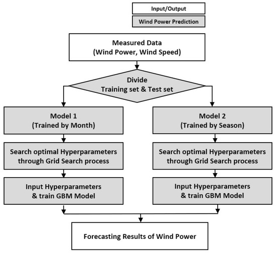
Figure 1.
Flow chart of the GBM forecasting model.
| Algorithm 1: Wind-power forecasting based on GBM algorithm | |||
| Input: 15 min interval data of Jeju Island | |||
| Data: wind speed (m/s) and wind power (MW) | |||
| 1 | Divide the training set and test set from the input data | ||
| 2 | for the test data do | ||
| 3 | select the last week (7 days) of the month | ||
| 4 | for the test data do | ||
| 5 | select the rest of the days of the month and seasons the test data are included | ||
| 6 | for each forecasting model | ||
| 7 | search for the optimal combination of the hyperparameters through the grid-search process | ||
| 8 | repeat for every forecasting model with different training datasets | ||
| 9 | until all the hyperparameter combinations in the grid are searched for | ||
| 10 | Insert the hyperparameters and train the GBM model | ||
| 11 | repeat | for every forecasting model with different training datasets | |
| 12 | until | all the forecasting-model forecasting results | |
| 13 | Evaluate the performance of the forecasting model by calculating the NMAE(%) value | ||
| end | |||
3. Results and Analysis
3.1. Results
3.1.1. Forecasting Results of the GBM Model
The following line graphs depict the forecasting results of the GBM (Figure 2, Figure 3 and Figure 4). The black lines with circles are the measured data of wind power, whereas the blue lines with an x mark represent the forecasted wind power.
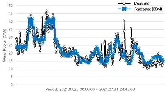
Figure 2.
Forecasting results of the GBM model trained by month (July).
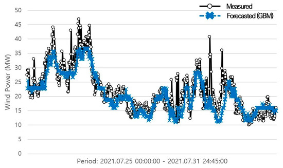
Figure 3.
Forecasting results of the GBM model trained by season (summer).
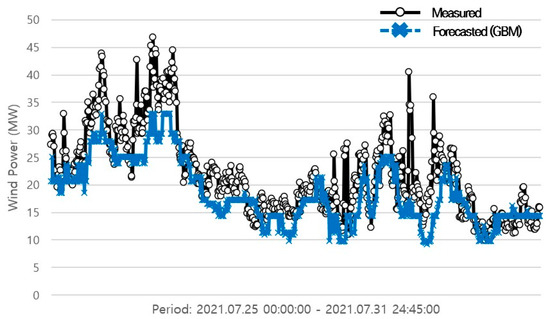
Figure 4.
Forecasting results of the GBM model trained by the previous month (long-term forecasting of one month ahead).
3.1.2. Analysis of Forecasting Results
The forecasting results of the GBM model were evaluated using performance metrics such as NMAE, MAE, and RMSE. The research emphazes NMAE since it is the standard metric used by the KPX (Korea Power Exchange) for calculating error rates to assess the “Incentives for Forecasting Accuracy of Renewable Generation” [20].
The forecasting model that only included data from July had an NMAE value of 5.1507%, an MAE value of 3.0904 MW, and an RMSE value of 4.1116 MW (Table 6). In contrast, the forecasting model that trained data for the whole summer had an NMAE value of 5.1933%, an MAE value of 3.1160 MW, and an RMSE value of 4.1657 MW. For long-term forecasting of one month ahead, the NMAE value turned out to be 6.9334%, whereas the MAE value was 4.1601 MW and the RMSE value was 5.4348 MW.
Table 6.
Performance evaluation of the GBM model.
A comparison was also made with the LSTM algorithm, which is one of the most frequent methods for predicting wind power. An identical test set was selected for both algorithms, 25 July and 25–26 July (Table 7). The GBM model trained by month had an NMAE value of 5.5354% for 25 July and 5.8716% for 25–26 July, demonstrating a better performance than the LSTM model, where each of its NMAE values were 7.5667% and 10.2290%, respectively. For the seasonally trained GBM model, the NMAE value was 4.7157% for 25 July and 5.4958% for 25–26 July. This is significantly lower than the NMAE of the LSTM model, where the values were 13.6782% and 11.6396%, respectively. Likewise, for both models trained by month and season, the GBM model also showed a better performance when comparing MAE and RMSE values.
Table 7.
Comparison of the GBM model with the LSTM model.
3.2. Grid-Security Analysis
3.2.1. Application to Jeju’s Power System
The forecasting results were applied to Jeju’s power system using PSS/E to conduct grid-security analysis. Cases for analysis were selected by standards based on the “General Terms and Conditions for Electricity Supply” provided by the Korea Electric Power Corporation (KEPCO). Unlike other regions in Korea, the on-peak period of Jeju Island ranges from 16:00 to 22:00 and does not vary by season [21].
Four cases during on-peak periods were chosen for the analysis because on-peak periods have the highest risk of instability in the power system (Table 8). The criterion for line fault was selected as 150% of loading, whereas the range of voltage limits varied from 0.95 to 1.05 p.u.
Table 8.
Cases in conducting the grid-security analysis.
3.2.2. Results of Grid-Security Analysis
The following table illustrates the results of the grid-security analysis (Table 9).
Table 9.
Results of grid-security analysis.
Load-flow calculations showed that all four cases reached tolerance within 20 iterations, leading to zero non-converged contingencies. Cases that applied average wind power off-peak from the forecasting models showed one flow violation in the system. In contrast, Case #1, which estimated the highest wind-power forecast (42.1144 MW) among all the cases, showed 148 high-voltage range violations and one flow violation. However, the maximum wind-power forecast of the seasonally trained model during off-peak showed the same results as the other two cases that demonstrated average wind power during off-peak.
4. Discussion
The following section underlines the key results of this paper. Considering that wind has a seasonal element, two types of GBM forecasting models were selected: One model had a training set including data from July, which was the same month as the test set. The other model selected its training set from the summer season, or June to August, involving data from the same season as the test set. In comparison, long-term forecasting was also performed, where the test set was a month ahead of the training set.
The monthly trained model showed slightly better accuracy in forecasts, achieving 5.1507% in NMAE, whereas the seasonally trained model showed an NMAE value of 5.1933%. Despite the advantage of possessing more training data, the input data from summer included more data points that had sufficient wind speed but had wind power converging to zero, hindering the accuracy of forecasting. The long-term forecasting model of the GBM algorithm had an NMAE value of 6.9334%, showing a less accurate result compared to short-term forecasting. It could be seen that a wide gap between the period of the training set and the test set may have decreased the accuracy in forecasting. To solve the inaccuracy of future inputs in the forecasting results, the GBM method’s deterministic forecasting results should be expanded to a probabilistic forecasting model. In addition, Figure 2, Figure 3 and Figure 4 which all depict the results of the GBM forecasting model, show that the model requires further advancement in precisely forecasting the peaks. This phenomenon may happen because the peaks in measured wind-power data represent high rarity, thus making it complicated for the GBM model to forecast the peaks precisely. Since the GBM method focuses on minimizing squared errors when building multiple regression trees, the total aggregation of these regression trees would be more effective in predicting data that closely resemble the general data contained in the training set. Hence, this threshold could be relieved by including data from the past years, enlarging the variety of the training set. Another approach for future improvements would involve calculating the average of various GBM models with a different set of training data.
Grid-security analysis concerning low-voltage range violations, high-voltage range violations, flow violations, and non-converged contingencies was performed to inspect whether the forecasted wind-power outputs have the possibility of disturbing the stability of the grid. Cases for performing the grid-security analysis include the following: the maximum and average wind power of the monthly and seasonally trained model. These cases were all selected from the on-peak periods, where the stability of the power system was the most vulnerable. From Table 9, only the case with the highest wind-power value resulted in 148 high-voltage range violations, whereas high-voltage range violations did not occur in the other three cases. It can be concluded that a bottom line for which the wind-power value causes high-voltage range violations existed between wind power in Cases #1 and #3.
5. Conclusions
Ongoing issues regarding climate change have attracted the attention of policymakers to increase the penetration of renewables all over the world. Although there is a global trend of expanding wind power, the intermittency of wind energy remains a significant issue for the integration of wind power into existing grids.
Therefore, this study focused on building a GBM-based wind-power forecasting model and analyzed the security of the grid when applying forecasting results. The monthly trained model achieved an NMAE of 5.1507%, showing the best accuracy in forecasting, along with the seasonally trained model with an NMAE of 5.1933% and the long-term forecasting model with an NMAE of 6.9334%. The GBM model also proved its outstanding performance compared to the LSTM algorithm, where the NMAE value for forecasting two days by both models trained by month and season was lower than the LSTM by approximately 5%.
Grid-security analysis of the selected four cases showed that only the case with the highest wind-power value resulted in 148 high-voltage range violations, whereas the other performances remained the same as the others. This indicates that further investigation would be able to discover the critical point where a certain amount of wind power results in high-voltage range violations.
Future research should expand the periods of the test set for various months and seasons of wind-power forecasting. To improve accuracy, a data-preprocessing step should be added to handle outliers in the input data and avoid the risk of high errors. Additional wind-turbine data, such as cut-in speed and wind-power data from previous years, as a control group, may help distinguish outliers. Moreover, the grid-search process for searching for the optimal hyperparameters should be continued to reduce the error rates of the model.
Author Contributions
Conceptualization, S.P. and J.H.; methodology, S.P.; software, S.P.; validation, S.P., J.L. and S.J.; formal analysis, S.P.; investigation, S.P.; resources, J.L. and S.J.; data curation, S.P.; writing—original draft preparation, S.P.; writing—review and editing, J.H.; visualization, S.P.; supervision, J.H.; project administration, J.H. All authors have read and agreed to the published version of the manuscript.
Funding
This research received no external funding.
Data Availability Statement
Not applicable.
Acknowledgments
This work was supported by the Korea Electric Power Corporation (No. R21XO01-1) and this work was supported by the National Research Foundation of Korea (NRF) grant funded by the Korea government (MSIT) (No. 2022R1F1A1074397).
Conflicts of Interest
The authors declare no conflict of interest.
References
- 2050 Carbon Neutrality Commission. 2050 Carbon Neutrality Scenario; Secretariat of the 2050 Carbon Neutrality and Green Growth Commission: Sejong, Republic of Korea, 2021; pp. 20–32. [Google Scholar]
- IRENA. Renewable Energy Statistics 2022; International Renewable Energy Agency: Abu Dhabi, United Arab Emirates, 2022; pp. 26–27. [Google Scholar]
- Cho, Y.S.; Cho, S.M.; So, J.Y.; Ahn, J.K.; Lee, S.H.; Kim, K.H.; Cho, I.H.; Lim, D.O.; Kong, J.Y.; Kim, S.K.; et al. CFI 2030 Plan Amendment Supplement Service; Jeju Special Self-Governing Province: Jeju, Republic of Korea, 2019; p. 17. [Google Scholar]
- Barthelmie, R.J.; Pryor, S.C. Climate change mitigation potential of wind energy. Climate 2021, 9, 136. [Google Scholar] [CrossRef]
- IRENA. Future of Wind: Deployment, Investment, Technology, Grid Integration and Socio-Economic Aspects; A Global Energy Transformation paper; International Renewable Energy Agency: Abu Dhabi, United Arab Emirates, 2019; p. 21. [Google Scholar]
- National Disaster and Safety Portal. Available online: http://www.safekorea.go.kr/idsiSFK/neo/sfk/cs/sfc/acd/iflccwUserList.jsp?menuSeq=99 (accessed on 18 November 2022).
- Chen, Q.; Folly, K. Wind power forecasting. IFAC-PapersOnLine 2018, 51, 414–419. [Google Scholar] [CrossRef]
- Soman, S.S.; Zareipour, H.; Malik, O.; Mandal, P. A review of wind power and wind speed forecasting methods with different time horizons. In Proceedings of the North American power symposium 2010, Arlington, TX, USA, 26–28 September 2010; pp. 1–8. [Google Scholar]
- IRENA. Innovation landscape brief: Advanced forecasting of variable renewable power generation; International Renewable Energy Agency: Abu Dhabi, United Arab Emirates, 2020; pp. 6–11. [Google Scholar]
- Choi, J.-G.; Choi, H.-S. Prediction of Wind Power Generation using Deep Learnning. J. Korea Inst. Electron. Commun. Sci. 2021, 16, 329–338. [Google Scholar]
- Biswas, A.K.; Ahmed, S.I.; Bankefa, T.; Ranganathan, P.; Salehfar, H. Performance analysis of short and mid-term wind power prediction using ARIMA and hybrid models. In Proceedings of the 2021 IEEE Power and Energy Conference at Illinois (PECI), Urbana, IL, USA, 1–2 April 2021; pp. 1–7. [Google Scholar]
- Ahmadi, A.; Nabipour, M.; Mohammadi-Ivatloo, B.; Amani, A.M.; Rho, S.; Piran, M.J. Long-term wind power forecasting using tree-based learning algorithms. IEEE Access 2020, 8, 151511–151522. [Google Scholar] [CrossRef]
- Singh, U.; Rizwan, M.; Alaraj, M.; Alsaidan, I. A machine learning-based gradient boosting regression approach for wind power production forecasting: A step towards smart grid environments. Energies 2021, 14, 5196. [Google Scholar] [CrossRef]
- Bankefa, T.; Biswas, A.K.; Ranganathan, P. Hybrid Machine Learning Models for Accurate Onshore/Offshore Wind Farm Forecasts. In Proceedings of the 2022 IEEE International Conference on Electro Information Technology (eIT), Mankato, MN, USA, 19–21 May 2022; pp. 335–341. [Google Scholar]
- Kuhn, M.; Johnson, K. Applied Predictive Modeling; Springer: Berlin/Heidelberg, Germany, 2013; Volume 26, pp. 203–206. [Google Scholar]
- Dhiman, H.S.; Deb, D.; Balas, V.E. Supervised Machine Learning in Wind Forecasting and Ramp Event Prediction; Academic Press: Cambridge, MA, USA, 2020; pp. 67–69. [Google Scholar]
- Natekin, A.; Knoll, A. Gradient boosting machines, a tutorial. Front. Neurorobotics 2013, 7, 21. [Google Scholar] [CrossRef] [PubMed]
- Hastie, T.; Tibshirani, R.; Friedman, J.H.; Friedman, J.H. The elements of statistical learning: Data mining, inference, and prediction; Springer: Berlin/Heidelberg, Germany, 2009; Volume 2, pp. 359–361. [Google Scholar]
- Greenwell, B.; Boehmke, B.; Cunningham, J.; Developers, G.; Greenwell, M.B. Package ‘gbm’. R package version 2022, 2.1.8.1. 2022, pp. 6–8. Available online: https://cran.r-project.org/web/packages/gbm/gbm.pdf (accessed on 27 November 2022).
- Korea Power Exchange (KPX). Available online: https://der.kmos.kr/intro/fr_intro_view10.do (accessed on 27 December 2022).
- Korea Electric Power Corporation (KEPCO) Marketing Division. Korea Electric Power Corporation (KEPCO). Available online: https://cyber.kepco.co.kr/ckepco/front/jsp/CY/D/C/CYDCHP00403.jsp (accessed on 27 November 2022).


Disclaimer/Publisher’s Note: The statements, opinions and data contained in all publications are solely those of the individual author(s) and contributor(s) and not of MDPI and/or the editor(s). MDPI and/or the editor(s) disclaim responsibility for any injury to people or property resulting from any ideas, methods, instructions or products referred to in the content. |
© 2023 by the authors. Licensee MDPI, Basel, Switzerland. This article is an open access article distributed under the terms and conditions of the Creative Commons Attribution (CC BY) license (https://creativecommons.org/licenses/by/4.0/).