An Efficient Variable Step Solar Maximum Power Point Tracking Algorithm

Abstract

The classic Photovoltaic system maximum power point tracking technique cannot concurrently take into account the dynamic response speed and steady-state accuracy when the light intensity changes. To address this issue, a new composite variable step MPPT control algorithm is developed in this study. Based on the three-stage variable step incremental conductance method, the algorithm adds the Kalman filtering algorithm to pre-process the photovoltaic cells output signal, and uses a new calculation approach to adjust the variable step coefficient. As a result, the perturbation step can be automatically modified according to changes in the external environment, which resolves the issues with poor dynamic reaction speed when the classic variable step algorithm started and the light changed. Compared to conventional MPPT control algorithms, the improved MPPT strategy can be easily realized using a hardware control system since it has a simplified control logic and requires less data to be calculated. In this study, the hardware circuit of the enhanced MPPT control algorithm is built using the ESP32 as the primary control chip. This chip can be utilized in conjunction with the Internet of Things to enable remote monitoring of the solar power system’s operational state. According to test results, the algorithm can instantly detect the maximum power point in all lighting circumstances with tracking accuracy of up to 99.6% and a reduction in dynamic response time of the system to 0.12 s.

1. Introduction

With its large reserves, lack of pollution, sustainable development, and other benefits, new energy is the subject of the majority of attention due to the rising importance of fossil energy pollution, limited reserves, and other challenges. Solar energy is green energy which is safer and more reliable than wind energy, and it has gradually become one of the hot spots of new energy development [1,2,3]. The link between light intensity and ambient temperature and the output power of solar cells is not linear, yet both factors have a significant impact. The maximum power point tracking algorithm has become a crucial component of photovoltaic power generation systems in order to increase their efficiency [4]. Photovoltaic power generation technology is a power generation technology that converts solar energy directly into electricity based on the photovoltaic effect of semiconductor materials. In 1839, the French scientist Becquerel was the first to discover the photovoltaic effect [5]. In 1954, Bell Laboratories in the United States used this principle to develop the first practical monocrystalline silicon solar cells [6,7]. Photovoltaic power generation technology has since entered the people’s vision.

The traditional MPPT control algorithms contain constant voltage method based on parameter selection, perturbation observation method based on sampling data and fixed-step conductance increment method. Among them, the control method of constant voltage method is easy to implement and the response speed is relatively fast, but it is not subjected to the influence of temperature and light intensity and cannot achieve global maximum power point tracking [8,9]. The perturbation observation method is a further improvement on the basis of the constant voltage method, but due to the characteristics of the algorithm itself, the output power of the photovoltaic cells cannot operate stably at the maximum power point, and is prone to misjudgment when the environmental conditions changed suddenly, thus falling into a local optimum [10,11]. In the traditional MPPT control algorithm, the conductance incremental method has the best control effect, but it cannot simultaneously take into account the tracking speed and steady-state accuracy, mainly because of the choice of the perturbation step. When a smaller perturbation step is chosen, the oscillation and energy loss near the maximum power point are weakened, but the number of perturbations needed to reach the maximum power point grow, which causes the problem of decreasing the response speed. On the other hand, when the bigger one is chosen, it can improve the tracking speed but the system will become extremely unstable [12,13].

To solve the above problems, Jiangguo Xu, Haixin Wang, and Karami proposed a variable step conductance increment method, which adjusts the perturbation step in real time according to the change in dP/dU so as to achieve improved tracking speed while reducing the oscillation loss [14]. However, the algorithm will have a very large change in dP/dU when the light intensity is suddenly changed, thus producing errors in the calculation of the perturbation step and aggravating the power oscillations [15]. Dong Mi, Thamer used a composite MPPT control algorithm based on conductivity increment and improved particle swarm algorithm [16,17], which improved the tracking accuracy of the system but when the environmental conditions changed, the particle swarm algorithm required a global search and the system was computationally intensive, thus reducing the response speed. In 2018, Chunjuan Liu proposed a photovoltaic multi-peak MPPT control algorithm based on the slime bacterium optimization algorithm [18], which calculated the search space generated by each weight and stochastic function by simulating the diffusion and foraging behavior of slime bacterium, so that the slime bacterium can perform the optimization search in any direction and in any step; although this algorithm can effectively avoid the effect brought on by the sudden change in light intensity, the data computation is large, which leads to the decrease in operation efficiency. In 2020, Zongyang Cui proposed a photovoltaic MPPT control method based on hybrid improved bat algorithm and fuzzy system [19]. When compared to the behaviors and traits of real creatures, it had a significant capacity for adaptation, but its execution was challenging because it called for the cooperative adjustment of multiple factors. Sabaripandiyan, D. added the control of the tracking scale factor to the variable step conductance increment method [20]. The algorithm can solve the contradiction between the response speed and steady-state accuracy, but the selection of its step adjustment coefficient S(k) is too complicated, and there is still some room for improvement.

This study suggested a novel composite MPPT control strategy based on the three-step variable step incremental conductance method with a new perturbation step calculation method and the Kalman filter algorithm, and created a matching hardware circuit to verify it in order to overcome the issues of the classic fixed step incremental conductance method and the current variable step incremental conductance method. The novelty and contribution of the article are summarized as follows:

• A first-order linear Kalman filtering algorithm is employed to pre-process the sensor detection data, which improves the stability and accuracy of the subsequent MPPT control algorithm.
• The calculation method of the step adjustment factor of the traditional variable step conductance increment is improved to increase the efficiency of the photovoltaic system.
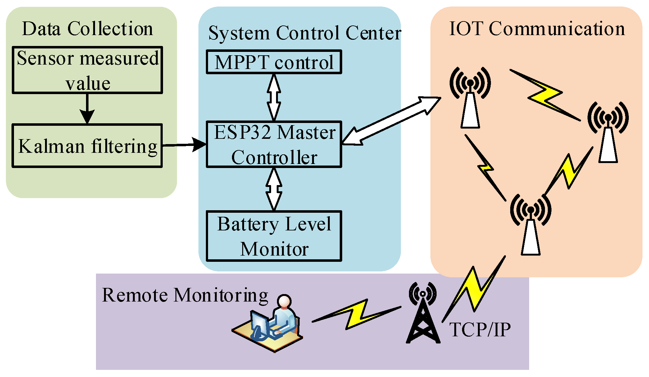
• The MQTT protocol is applied to transmit information when the photovoltaic system is in operation, and the corresponding client is designed to remotely monitor the working status of the photovoltaic cells.

2. Photovoltaic Mathematical Model and Output Characteristics Analysis

The photovoltaic effect of the semiconductor PN junction is the basis of the operation of photovoltaic cells, and Figure 1 illustrates this operation. When a semiconductor PN junction is exposed to light, the internal atoms release electrons, creating corresponding hole–electron pairs. As a result, under the influence of the potential electric field, the electrons diffuse to the N region and the holes diffuse to the P region, forming a photovoltaic electric field in the PN junction region [21,22]. After the interaction between the photo-generated electric field and the potential electric field, there is a positive charge in the P area and a negative charge in the N region; at this moment, a photo-generated current will be generated if an external load is connected to form a circuit.

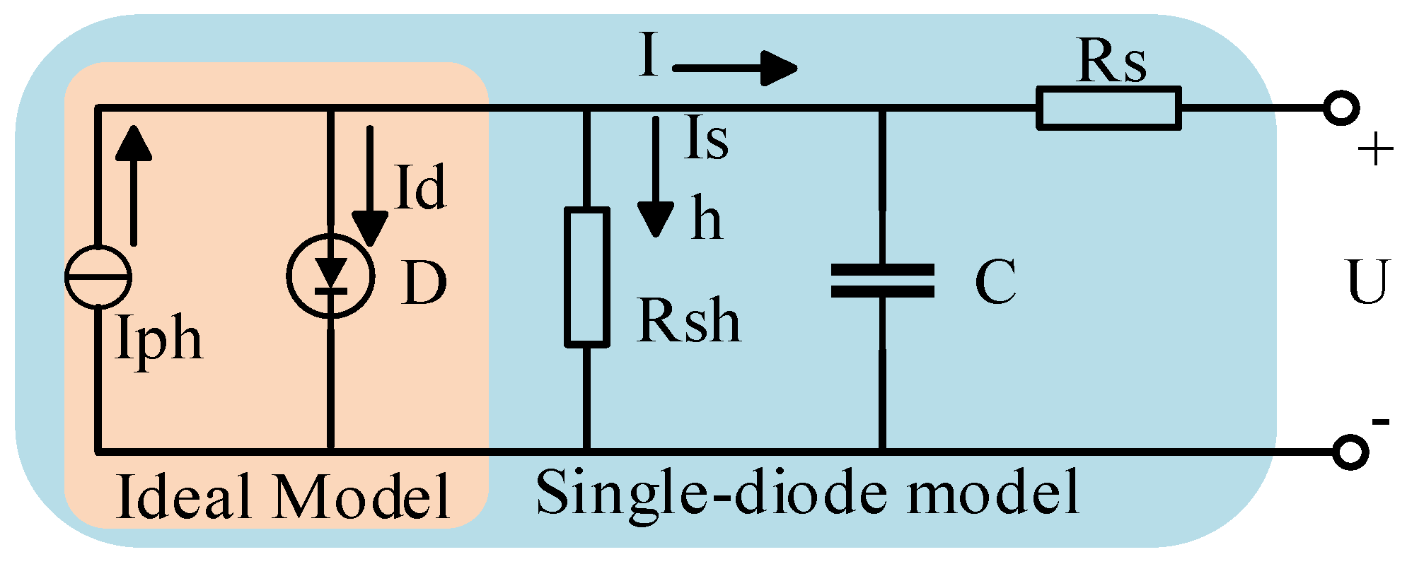
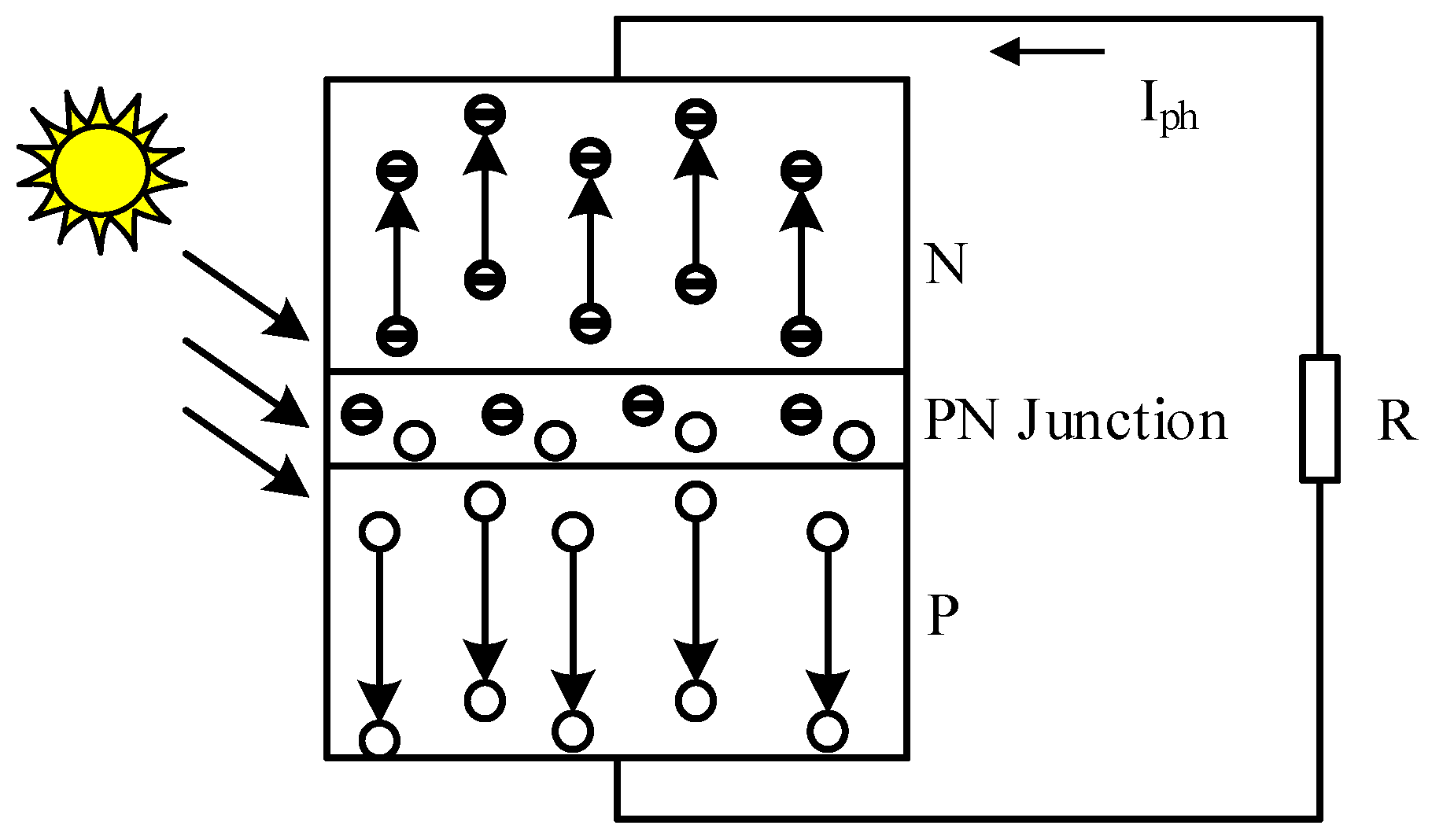
2.1. Photovoltaic Cell Mathematical Modeling and Analysis

The photovoltaic cells are the core part of the whole photovoltaic system which is analyzed by the ideal model or single diode equivalent circuit model and the structure is shown in Figure 2.

As shown in Figure 2, according to the Kirchhoff’s voltage–current law,

$$I=I_{ph}-I_d-I_{sh},$$

(1)

$$I_{sh}=(U+I{R}_s)/R_{sh}.$$

(2)

The equivalent volt-ampere characteristic equation for the single diode model of the photovoltaic is defined as (3):

$$I=I_{\mathrm{ph}}-I_0[\exp (\frac{q(U+I{R}_s)}{AKT})-1]-\frac{U+I{R}_s}{R_{sh}},$$

(3)

where I_ph is a photo-generated current whose magnitude varies with temperature and light intensity, I₀ is the reverse saturation current of the diode, I_d is the current flowing through the diode, I_sh is the current flowing through the shunt resistor R_sh, q is the electronic charge, I and U are the output current and output voltage of the solar cells, respectively. A is the ideal factor of the diode, T is the absolute temperature value when the photovoltaic cells is operating, and K is Boltzmann’s constant, which is defined in (3).

In practical use, Formula (3) can be simplified to (4):

$$I=I_{\mathrm{sc}}[1-B\times (\exp (U/({\mathrm{CU}}_{\mathrm{oc}}))-1)].$$

(4)

When using MATLAB to model and analyze (4) under standard conditions (STC, S = 1000 W/m², T = 25 °C), it requires further simplification. The mathematical model required for its simulation model can be (5)~(10), and the meanings of the symbols are shown in

Table 1. Explanation of Symbols (5)–(10).

Symbol	Quantity	Units
tref	Ambient temperature under STC	°C
Sref	Light intensity under STC	W/m2
Isc	Short Circuit Current	A
Uoc	Open Circuit Voltage	V
a	0.00255	°C
b	0.5	\
c	0.00288	°C

.

$$\mathsf{\Delta }t=t-t_{ref},$$

(5)

$$\mathsf{\Delta }s=s/s_{ref}-1,$$

(6)

$$I_{sc}^{\prime }=I_{sc}(s/s_{ref})(1+a\mathsf{\Delta }t),$$

(7)

$$U_{oc}^{\prime }=U_{oc}(1-c\mathsf{\Delta }t)\ln (e+b\mathsf{\Delta }s),$$

(8)

$$I_m^{\prime }=I_m(s/s_{ref})(1+a\mathsf{\Delta }t),$$

(9)

$$U_m^{\prime }=U_m(1-c\mathsf{\Delta }t)\ln (e+b\mathsf{\Delta }s).$$

(10)

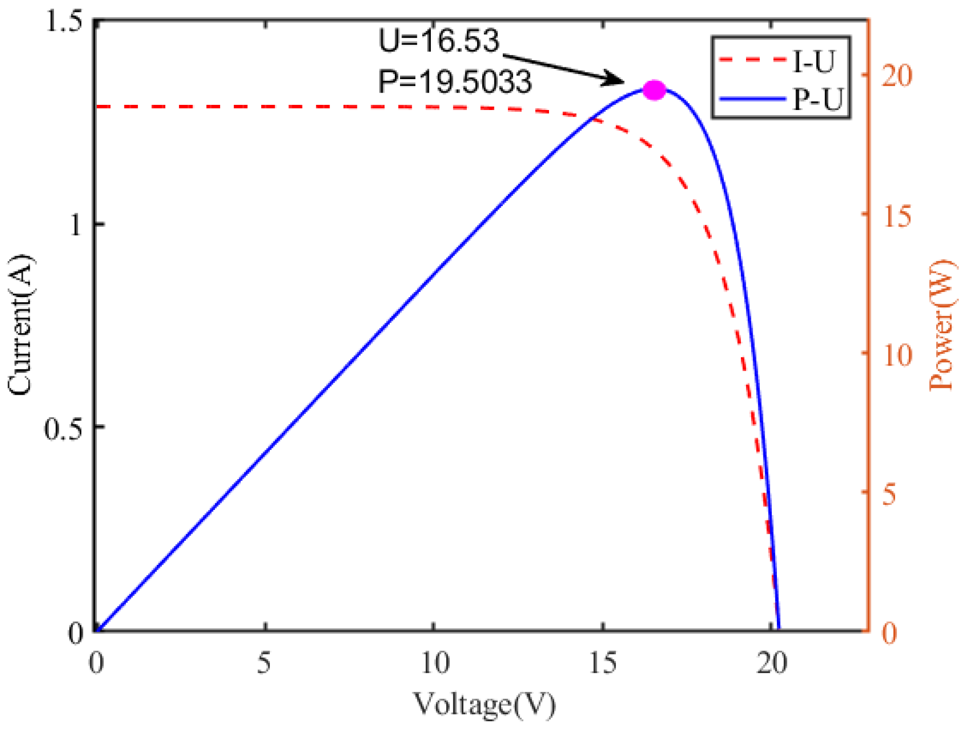
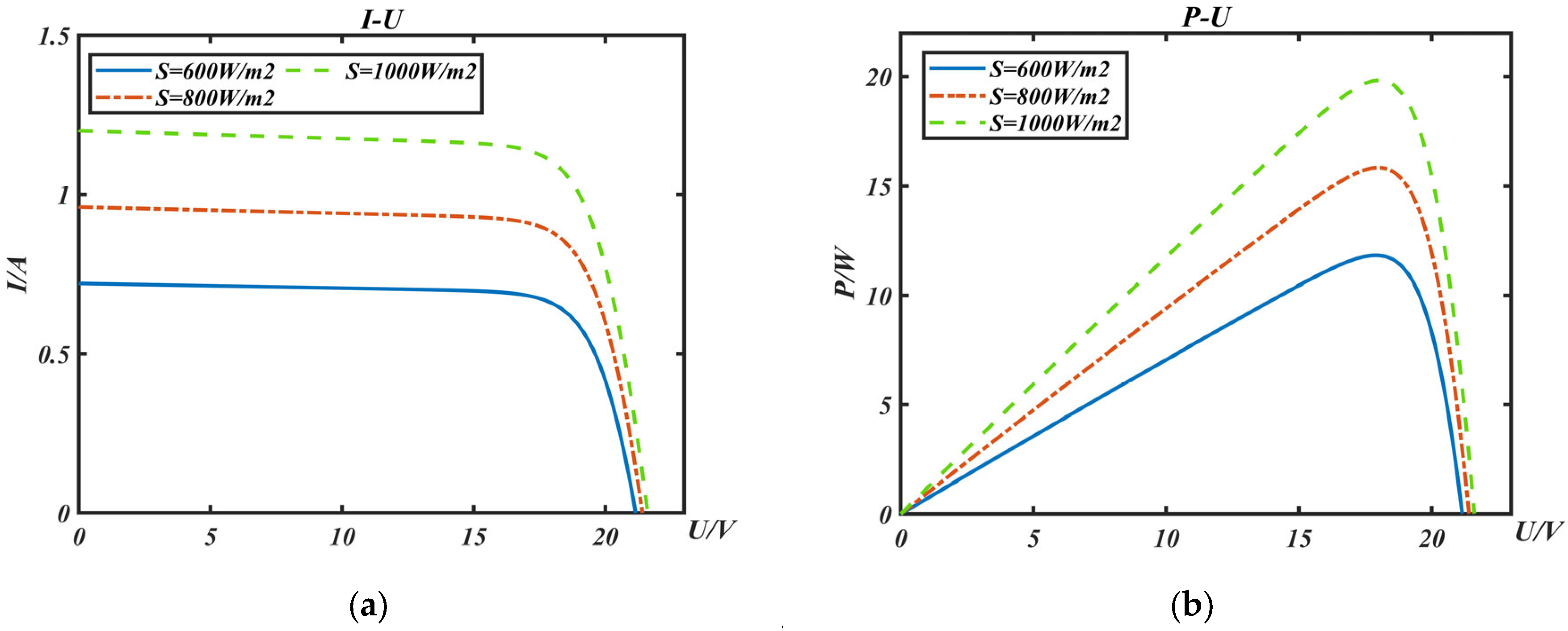
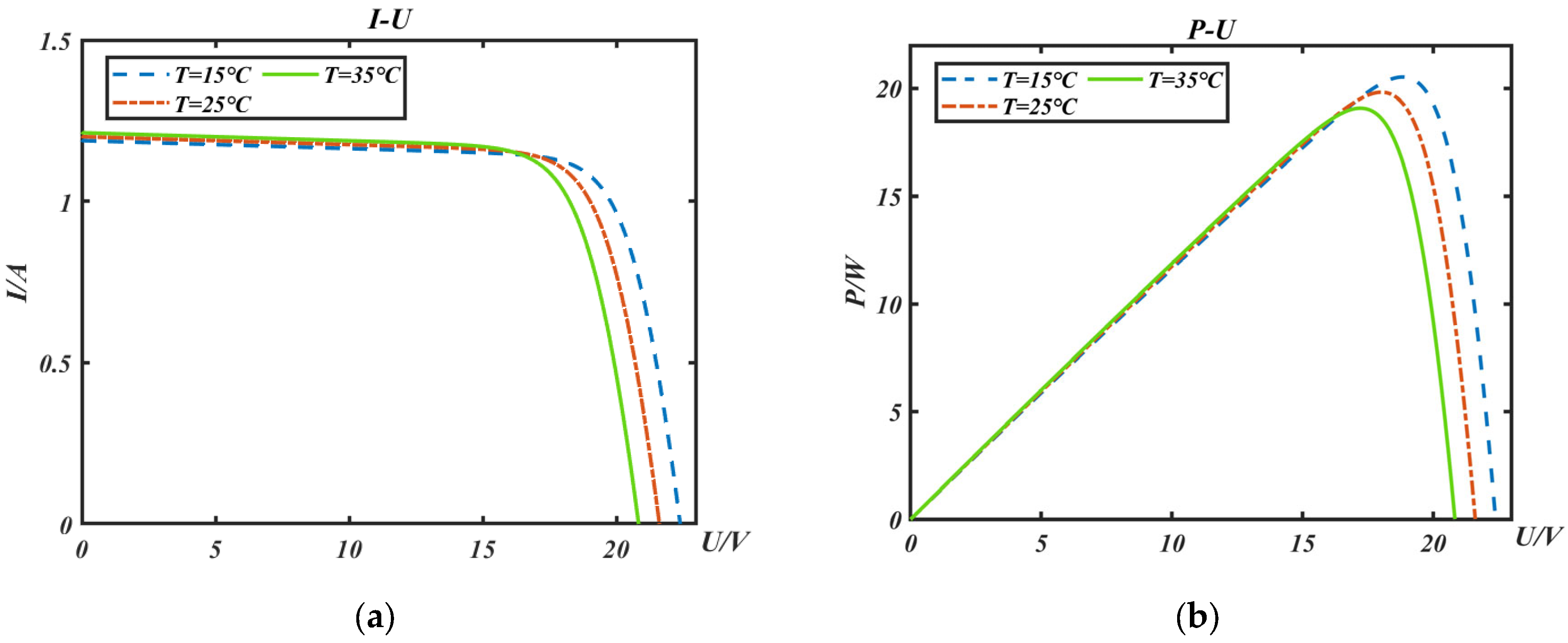
2.2. Photovoltaic Cell Output Characteristics Analysis

Through the photovoltaic cell mathematical model established in the previous section, the standard state T_ref = 25 °C, light intensity S_ref = 1000 W/m², short-circuit current I_sc = 1.2 A, open-circuit voltage U_oc = 21.6 V, maximum power current I_m = 1.1 A, and maximum power voltage U_m = 18 V. According to this parameter, to build the MATLAB simulation model, the P-U and I-U output characteristic curves of the single solar panel used are shown in Figure 3. As shown by the P-U characteristic curve in Figure 3, when the light intensity and temperature of the environment in which the photovoltaic cells are located are fixed values, its output power is a curve that varies with the output voltage, and its change law is first increasing and then decreasing, and there is a unique maximum point, which is the maximum power point [23]. When the surrounding environmental conditions changes, the value of the maximum power point also changes; in order to make the photovoltaic cells always work in the best condition, it is necessary to implement the strictest power point tracking control algorithm [24].

To further analyze the effects of light intensity and environment temperature on the output characteristics of photovoltaic cells, first, the ambient temperature was set to 25 °C and the light intensity was increased from 2000 W/m² to 3000 W/m² in steps of 500 W/m² to obtain the curve of the effects of light intensity on the output characteristics of photovoltaic cells. Then, the light intensity was set to 2000 W/m² and the ambient temperature increased from 25 °C to 35 °C in steps of 5 °C to obtain the curve of the effect of ambient temperature on the output characteristics of photovoltaic cells [25,26].

As can be seen from Figure 4, the output characteristic curve of photovoltaic cells under the same light intensity shifts downward at the maximum power point and shifts leftward at the open circuit voltage U_oc with the increase in temperature, and the temperature has an obvious effect on the open circuit voltage. While the output characteristic curve in the linear region of constant current source is not much changed by temperature, the short-circuit current I_sc is only slightly increased with the increase in temperature.

Figure 5 illustrates the way in which the output characteristic curve of photovoltaic cells at the same temperature shifts the maximum power point upward with an increase in light intensity, increases the short-circuit current with an increase in light intensity, and slightly increases the open-circuit voltage U_oc.

In practical use, solar panels may also be affected by the external environment with partial shading conditions (PSC), and thus the photovoltaic cells P-U characteristic curve appears as shown in Figure 6 with a multi-peak problem, where a global maximum power point (GMPP) and numerous local maximum power points (LMPP) exist. In order to ensure the power generation efficiency of the photovoltaic power system, the MPPT algorithm should be able to solve the photovoltaic output multi-peak problem under different situations, so that the system output always runs at GMPP [27,28,29].

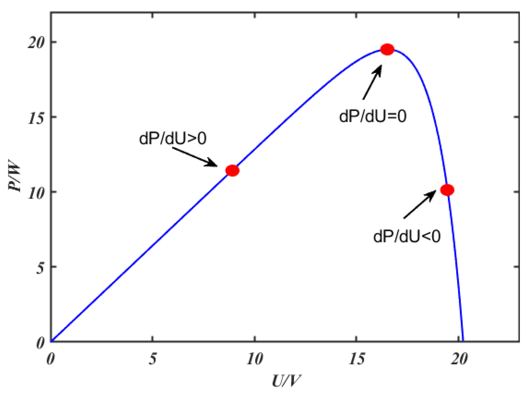
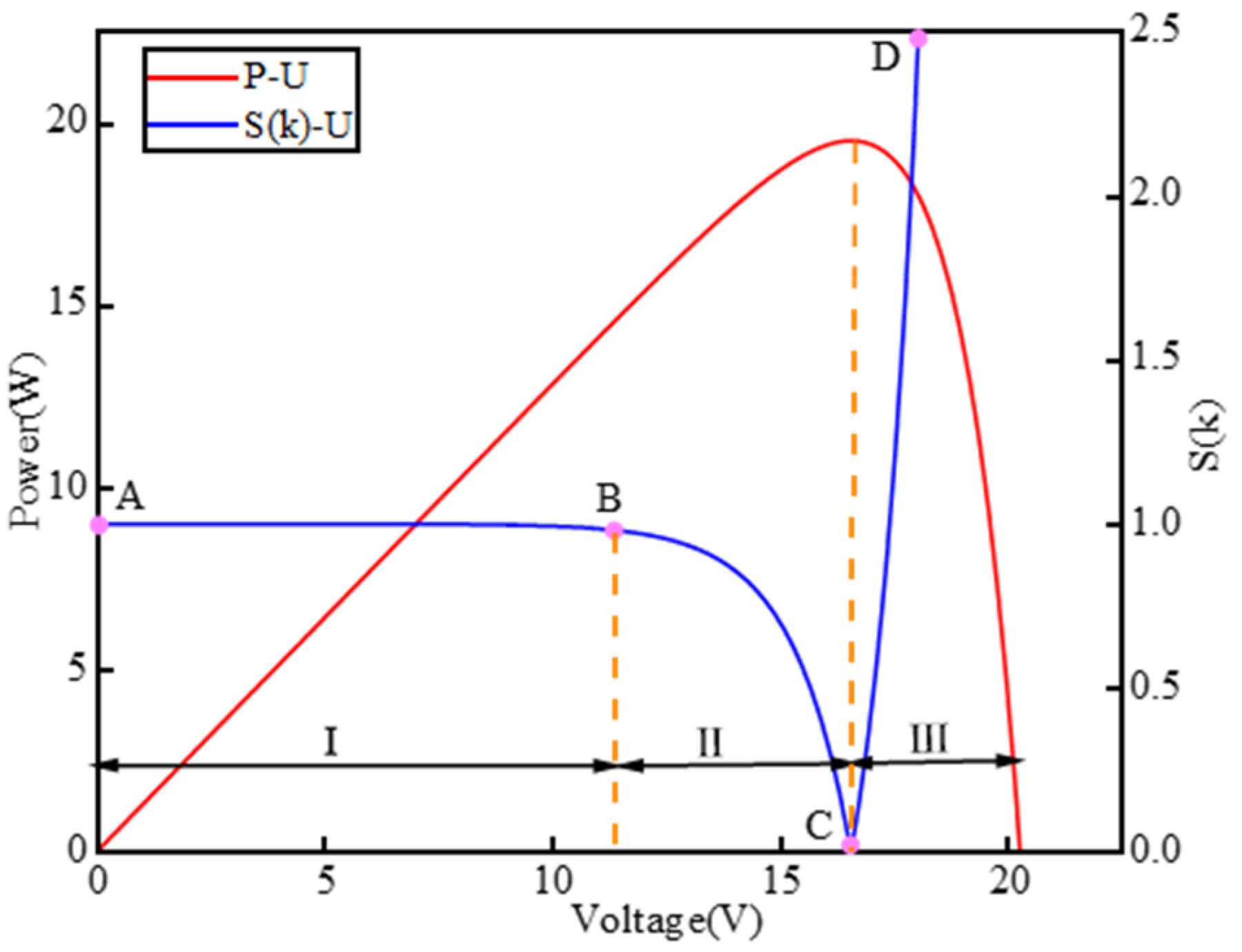
3. MPPT Control Principle Analysis

Through the analysis of the simulation results of the photovoltaic cells output characteristics, it can be seen that the photovoltaic cells output characteristics are non-linear in Figure 4, Figure 5 and Figure 6. The output power of photovoltaic cells does not increase continuously with the increase in output voltage; it has only one maximum point under certain conditions. At the maximum point of photovoltaic cell output power, when the output voltage continues to increase, the output current and output power of photovoltaic cells will drop rapidly, and factors such as light intensity, ambient temperature and load conditions will have an impact on it [30,31,32]. The light intensity has a large impact on the output current of photovoltaic cells; the output current increases with the increase in light intensity, the temperature has a large impact on the output voltage of photovoltaic cells, the open circuit voltage decreases with the increase in temperature, and the change in load affects the responsiveness of photovoltaic power generation system. In order to make full use of the energy converted by the photovoltaic cells to improve the energy utilization of the whole system, the photovoltaic cells are always required to be in the maximum power output state. Therefore, a maximum power point tracking control device is needed to be added between the photovoltaic panel and the load so that the photovoltaic power system can track the maximum power point in real time [33]. To facilitate the simulation analysis, the MPPT control principle can be referred to the maximum power transfer theorem of linear DC power supply, and the established photovoltaic cells equivalent model is shown in Figure 7.

The power consumed by the load R₀ is expressed as (11):

$$P=I^2{R}_o={(\frac{U_i}{R_i+R_o})}^2\times R_o,$$

(11)

U_i and R_i be constants and the value of R₀ be a variable, which the formula (11) calculated for (12) and (13) by obtaining the first-order and second-order derivative of R₀:

$$\frac{dP}{d{R}_o}=U_i^2\times \frac{R_i-R_o}{{\left(R_i+R_o\right)}^3},$$

(12)

$$\frac{d^{2}P}{d{R}_o^2}=2U_i^2\times \frac{R_o-2R_i}{{\left(R_i+R_o\right)}^4}.$$

(13)

According to (12), the power consumed by the load has only one extreme value point, when R_i = R₀ and d²(P)/d($R_0^2$) < 0, at which time the load can obtain max power transmission. Buck converter is a dc-dc with lower voltage, while boost is a dc-dc converter with higher voltage. In this paper, the output voltage of solar panels is approximately 15 V, so the buck converter is used to charge lead acid batteries. In order to achieve maximum power matching, the photovoltaic cells have been output at maximum power, where the photovoltaic array and the load can be connected to a buck circuit to change the equivalent resistance of the external load in real time to make sure the internal resistance of the solar panel is matched to maximum power transfer [34]. The maximum power transfer structure of the photovoltaic cells is shown in Figure 8.

In order to estimate the photovoltaic cell maximum power point under the present environmental conditions, the MPPT control strategy uses real-time measurements of their output power. It then uses the appropriate control algorithm to satisfy the maximum power point need by adjusting the load voltage and current values [35]. Regardless of the changes in external environmental conditions, the system automatically tracked the current optimal operating point in real time through the MPPT technique, thus improving the conversion efficiency of the photovoltaic power generation system.

4. Traditional Conductance Increment Method Analysis

The MPPT control technique for tracking used in the conductance increment method is primarily based on the correlation between the instantaneous conductance and the rate at which the conductance of the photovoltaic cells changes. Figure 9 demonstrates this; when the light intensity is constant, one power point at its maximum is available, and the sign of dP/dU is different on both sides of the maximum power point, and dP/dU = 0 at the maximum power point. The first order derivative of the output power of the photovoltaic cell is defined in (14).

$$\frac{dP}{dU}=\frac{d(IU)}{dU}=I+\frac{dI}{dU}U.$$

(14)

When dP/dU = 0, the output power of the photovoltaic cells reaches its maximum value, which can be expressed in (14) as dI/dU =−I/U. The rules for calculating the perturbation step update of the fixed-step conductance increment method are shown in (15). ΔU = U(t) − U(t − 1); on the left side of the maximum power point, dI/dU > −I/U, the disturbance voltage ΔU should be increased so as to fasten into the maximum power point as soon as possible. On the right side of the maximum power point, dI/dU < −I/U, the open circuit voltage should be smaller so as to approach the maximum power point.

$$\left\{\begin{array}{ll}U(\mathrm{k}+1)=U(\mathrm{k})+\mathsf{\Delta }U& ,dI/dU>-I/U\\ U(\mathrm{k}+1)=U(\mathrm{k})& ,dI/dU=-I/U\\ U(\mathrm{k}+1)=U(\mathrm{k})-\mathsf{\Delta }U& ,dI/dU<-I/U\end{array}\right..$$

(15)

The traditional conductance increment method performs well in solving the single-peak photovoltaic model under uniform light intensity, but under local shading conditions, the P-U output characteristic curve of the photovoltaic system is no longer a single-peak model, and the continued use of the traditional MPPT control algorithm tends to fall into a local optimal solution, leading to a reduction in the overall power generation efficiency of the photovoltaic system [36,37]. The variable step incremental conductance method is an improved method which can solve the fixed step proposed control strategy by establishing the relationship between step size and power voltage, decreasing the step size to improve tracking accuracy when the system is nearing the maximum power point and increasing the step size to improve tracking speed when the system is moving away from the maximum power point. This allows the system to achieve the goal of quick response and high stability.

For the constant step conductance increment method, choosing a larger perturbation step can improve the tracking speed, but the power loss at steady state is more, and a smaller perturbation step can improve the steady-state tracking accuracy, but it will slow down the tracking speed [38]. This research suggested an improved three-step variable-step conductance increment technique MPPT control using Kalman filter algorithm to resolve the conflict between the dynamic speed and steady-state accuracy of the photovoltaic system induced by the step selection.

5. Design and Validation of an Improved Three-Stage Variable Step Incremental Conductivity Method

Figure 10 depicts the general architecture of the MPPT control system based on the Kalman filter technique [39,40], which is mainly divided into four parts: data acquisition module, system master control module, IOT communication module, and long-distance monitoring module. The system is based on DHT11 ambient temperature and humidity sensor, BH1750 light intensity sensor and INA226 power detection IC, which detected the temperature and humidity, light intensity and output voltage and current of the environment around the solar panel, respectively. Moreover, it adopts the ADC pin of ESP32 to monitor the battery power, and the NTC thermistor to detect the temperature of the main control PCB.

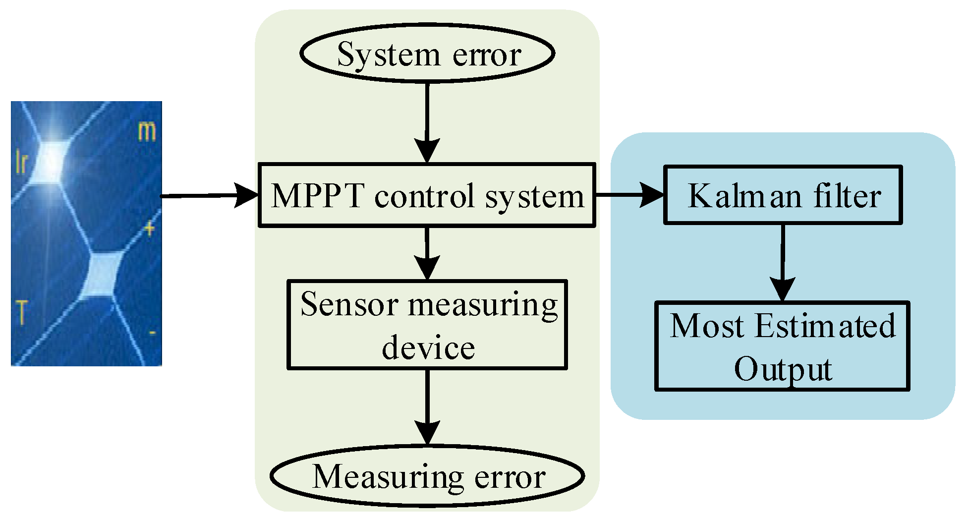
5.1. Principle of Kalman Filter Algorithm

The sensors may be affected by system noise and measurement noise during operation, which may lead to abnormal measurement data and carry coarse errors, resulting in poor system control [41]. To solve the problem of large fluctuations in sensor measurement data, a first-order Kalman filtering algorithm is used to preprocess the voltage and current data from the PV cells output to improve the control accuracy of the system.

Kalman filtering is an optimal recursive numerical processing algorithm that occupies little program memory space, responds quickly, and is well suited for applications in real-time data processing. The characteristics of systems of the Kalman filter algorithm are the following: there is no perfect mathematical model of the system or the system model difficult to build, system perturbations are uncontrollable, and errors exist in the sensor measurements of the system [42,43,44]. In essence, filtering is a process of signal processing and transformation, which can be implemented either in hardware or in software. By updating the estimations of the state variables with the estimates from the previous instant and the observations from the present moment, Kalman filtering is a type of software filtering technique that uses the least mean square error as the optimum estimation criterion [45,46,47]. The framework of the Kalman filtering algorithm applied in the MPPT control algorithm is as shown in Figure 11.

For the convenience of system modeling and program writing, it is reasonable to assume the following: the state transition process of the system can be described as a discrete-time stochastic process, the system state is influenced by the control input, neither the system state nor the measurement process is immune to noise, and the system state is not directly observable [48]. Based on the above assumptions, the core formulas of the established Kalman filtering algorithm can be expressed as (16) to (20), and their symbolic meanings are shown in

Table 2. Explanation of Symbols (16)–(20).

Symbol	Quantity
A	State shift matrix
B	Input control matrix
H	Observational model matrix
Pk	Error covariance matrix
Q	Process noise covariance matrix
R	Measurement noise covariance matrix
I	Unit matrix
K	Kalman gain
-	represents the priori value
^	represents the estimated value

.

$${\widehat{X}}_k^{-}=A{\widehat{X}}_{k-1}+B{\widehat{U}}_{k-1},$$

(16)

$$P_{\mathrm{k}}^{-}=A{P}_{k-1}{A}^T+Q,$$

(17)

$$K_k=P_{\mathrm{k}}^{-}{H}^T{(H{P}_{\mathrm{k}}^{-}{H}^T+R)}^{-1},$$

(18)

$${\widehat{X}}_k={\widehat{X}}_k{}^{-}+K_k(Z_k-H{\widehat{X}}_k^{-}),$$

(19)

$$P_k=(I-K_{k}H)P_{\mathrm{k}}^{-}.$$

(20)

From the above equations, it is determined that the Kalman filter consists of two main components: prediction and correction. The prediction process is mainly employed to calculate the prior estimates of the current state using the update equation, to derive the values of the current state variables and the error covariance estimates, and to construct the prior estimates for the next moment state. The main task of the correction process is to return information about the iterations of the system and to build posteriori estimates of the current state using the prior estimates of the prediction update equation in the prediction process and the current prediction [49,50].

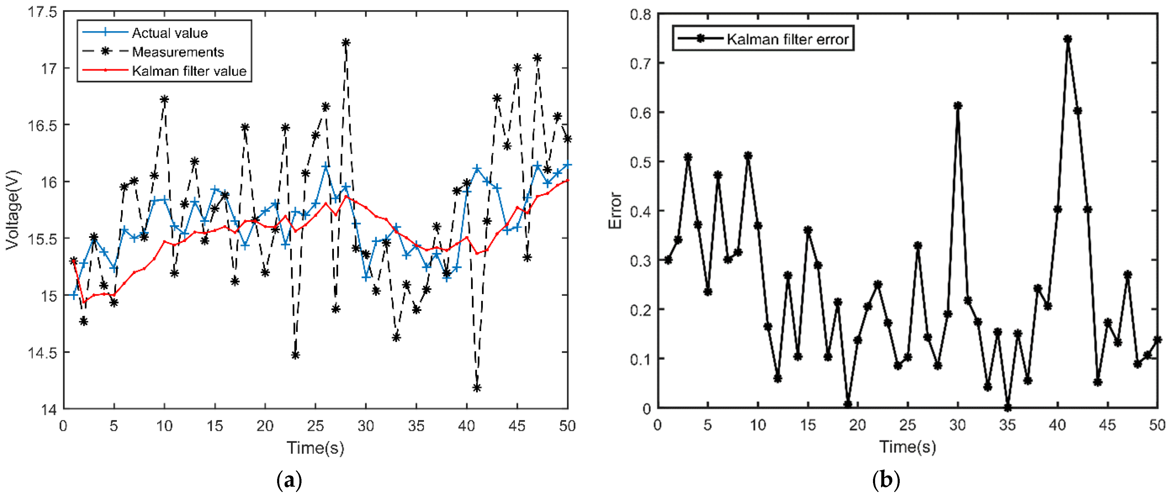
5.2. Processing of Photovoltaic Cell Output Information by Kalman Filtering Algorithm

Under the ambient conditions of light intensity of 56,000 W/m² and 38 °C, the photovoltaic cell output voltage and current are detected in real time by INA226 power detection IC, and the collected information is transmitted into the Kalman filter for data pre-processing. In the process of Kalman filter algorithm parameter rectification, the process covariance matrix Q is 0.05 and the measurement noise covariance matrix R is 0.5. The photovoltaic cell output voltage after Kalman filter real-time processing effect is shown in Figure 12a, the error curve is shown in Figure 12b. The photovoltaic cell output current after Kalman filtering real-time processing effect is shown in Figure 12c, the error curve is shown in Figure 12d. After calculating, the average error between the sensor value and the real value after Kalman filtering is 0.23, and the average error between the real-time sensor detection value and the real value is 0.55. Using Kalman filtering algorithm, the sensor measurement error is reduced to 32%, which effectively improves the control accuracy of the system.

Figure 12 illustrates the ways in which the Kalman filter technique is used to pre-process the sensor measurement data and successfully address the issue of significant variations in the sensor data measured, and the data processing speed is high without generating large time lags, which plays a good pre-processing role for the subsequent MPPT control algorithm. In the process of conducting the system dynamic simulation, random noise is added to analyze the effect of sensor measurement error on the system response. When a large noise is suddenly added, the Kalman filtered output does not change suddenly due to the existence of the cumulative error part of the system. In addition, when the system model and observation mode are reasonable, the Kalman filtered part can be approximated as a real-time system.

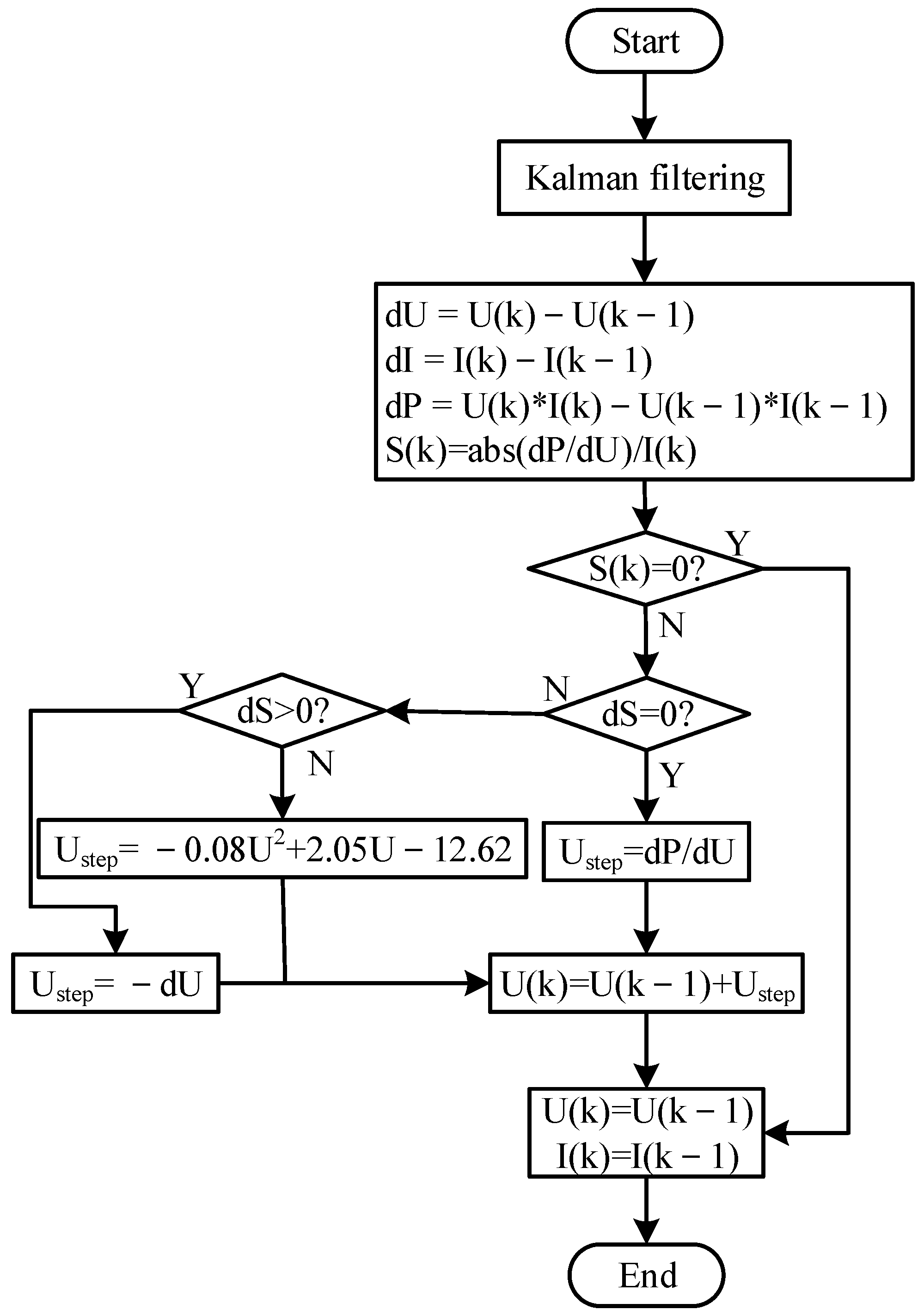
5.3. Improved MPPT Control Algorithm by Kalman Filter

The conventional variable step algorithm relies on the differentiation of the photovoltaic cells output power and voltage to adjust the step size, but the variation in dP/dU varies greatly under different light intensities, and an optimal speed factor cannot be determined to meet the need of maximum power tracking under the conditions of drastic light changes. Equation (14) showed that the power–voltage differential curve depended on the output current of the photovoltaic cells, which had different values for different light intensities, and to eliminate this variability, a step adjustment factor S(k) was introduced. The S(k) output characteristic curve is shown in Figure 13 under the ambient conditions of light intensity of 1000 W/m² and temperature of 25 °C.

At the maximum power point, the value of S(k) is zero. With the increase in voltage, the value of S(k) is first approximated as a constant in the part of the P-U curve with slope greater than zero, and then rapidly decreases to zero. With the continuous increase in voltage, the value of S(k) increases exponentially in the part of the P-U curve with slope less than zero. Based on this law, the maximum power point is used as a divider to divide S(k) into three parts, I, II, and III, each of which is perturbed in a different step. According to the reference [18], a three optional step conductance increment approach based on the step adjusting factor S(k) is suggested, and the step update rule of this algorithm is shown as follows:

$$U(k)=U(k-1)\pm S(k),$$

(21)

$$S(k)=\frac{1}{I(k)}\left|\frac{\mathrm{d}P}{\mathrm{d}U}\right|=1+\frac{U(k)}{I(k)}\left|\frac{\mathrm{d}I}{\mathrm{d}U}\right|.$$

(22)

In this algorithm, setting a queueing upper limit N_max and queueing lower limit N_min for S(k), if S(k) ≥ N_max, the step size is chosen as ΔU_max; if N_min < S(k) < N_max, the step size is chosen as ΔU; if S(k) ≤ N_min, the variable step adjustment is used, and the step size is chosen as S(k) × ΔU. This method can automatically adjust the variable step size according to the change in light intensity region, which can still maintain good dynamic tracking speed and steady-state accuracy when the light intensity is changing rapidly. However, the determination of the step adjustment coefficient S(k) is too complicated, and the upper and lower limits of S(k) will change under different light intensities, which may result in the local optimal point serving as the operating point of tracking rather than the global power quality improvement. To solve this problem, combined with the characteristics of S(k) curve in Figure 13, this study suggests a new step update rule, and Figure 14 illustrates the control flow of its enhanced integer variables step conductance increment approach. In order to locate the maximum power point under the current conditions, it is first necessary in practical applications to gather the filtered PV cell output voltage and current using a power sensor, store the sensor data at the current moment into an array, and compare it with the state value at the previous moment. The purpose of tracking the maximum power point is then accomplished by adjusting perturbation step S(k) by computing the change in voltage and power.

$$U(k)=U(k-1)+U_{step},$$

(23)

$$U_{step}=\left\{\begin{array}{ll}dP/dU,& \mathsf{\Delta }\mathrm{S}=0\\ -0.08U^2+2.05U-12.62,& \mathsf{\Delta }\mathrm{S}<0\\ -\mathsf{\Delta }U,& \mathsf{\Delta }\mathrm{S}>0\end{array}\right..$$

(24)

Figure 15 shows the method simulation model of the modified three-stage variable step incremental conductance method, using the photovoltaic cells and circuit parameters shown in

Table 3. PV Module and Circuit Parameters.

Parameters	Values
Maximum Power	19.8 W
Open circuit voltage (Voc)	21.6 V
Short-circuit current (Isc)	1.2 A
Voltage at maximum power point (Vmp)	18 V
Current at maximum power point (Imp)	1.1 A
Filter Capacitor (C)	47 uF
Load resistance (R)	1 K
Power Inductor (L)	6.8 uH

. In order to make the system more responsive, the switching frequency of PWM is set to 10 KHz, and all components are ideal during the simulation. The output capacitor is linked at the load side and the input capacitors are connected between the photovoltaic panels and the DC-DC converter in order to reduce input ripple voltage and filter ripple current, so as to ensure the stability of the system operation. Schottky diodes (V_f = 550 mV, I_o = 3 A) are selected as current continuity diodes in the Buck converter to protect the components from damage by induced voltage.

6. Hardware Circuit Design for MPPT Control

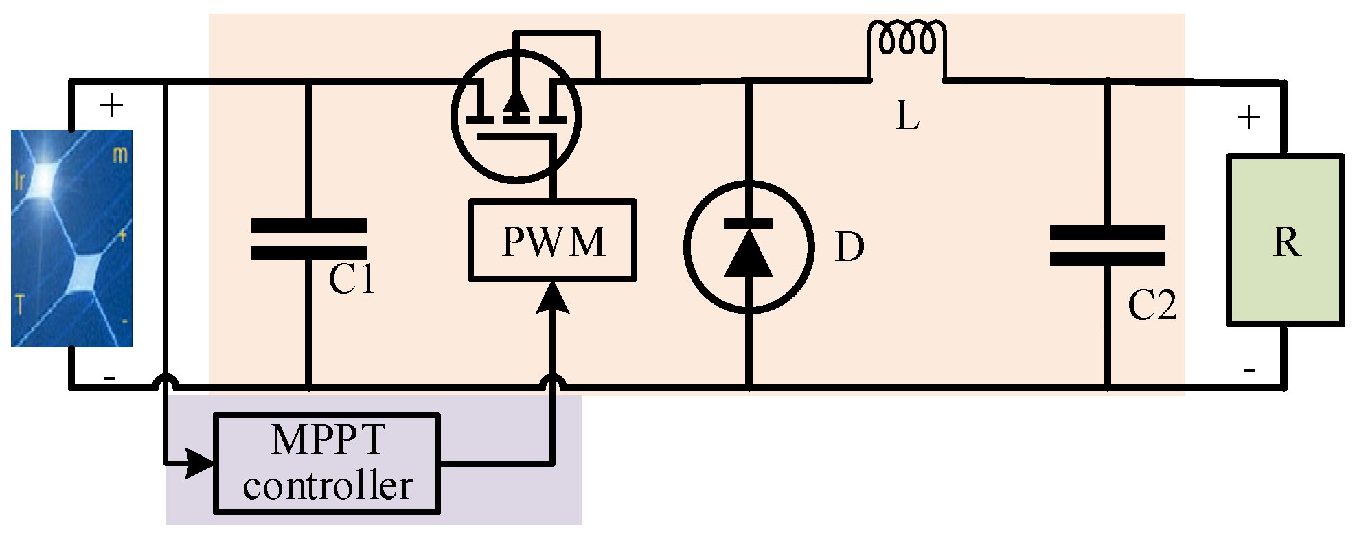
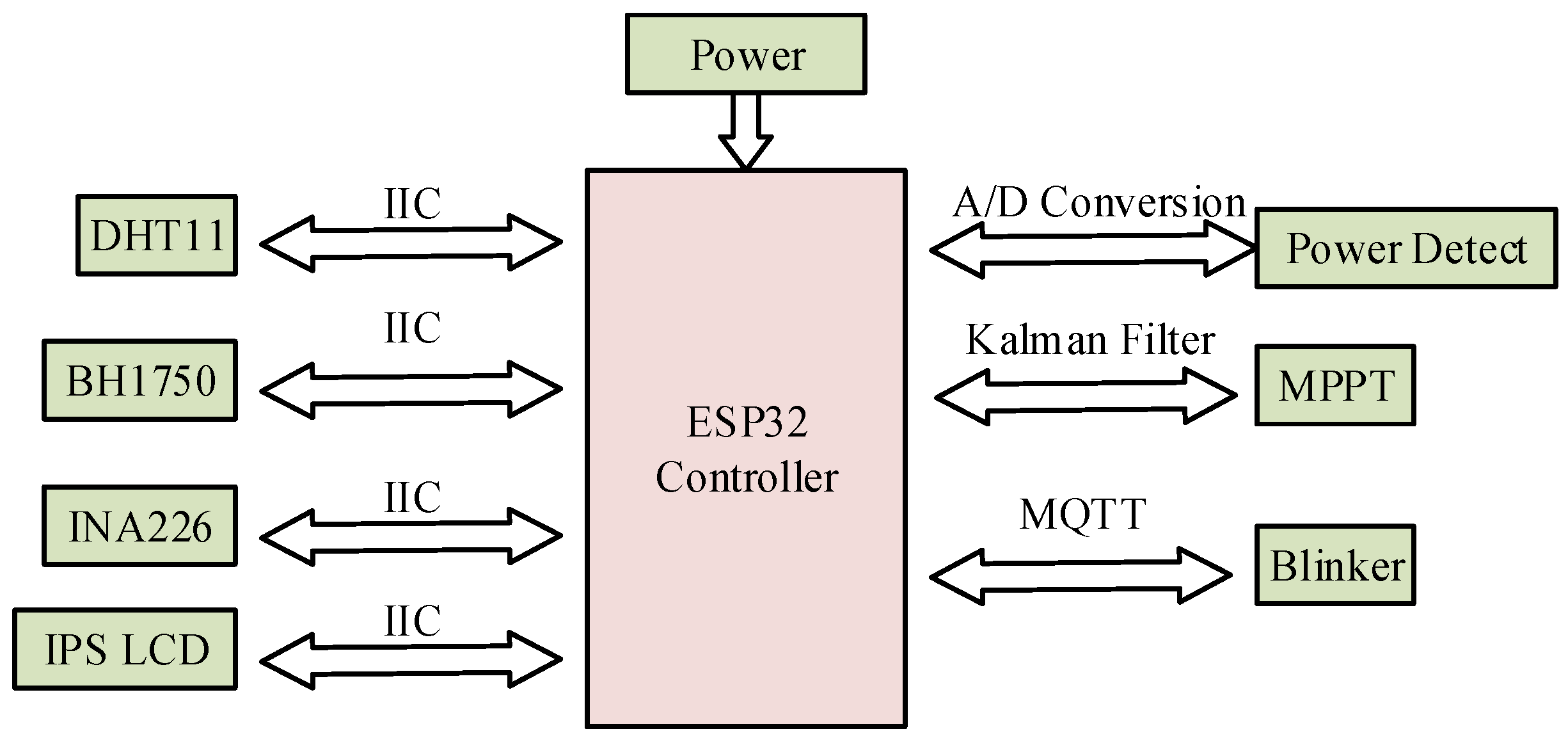
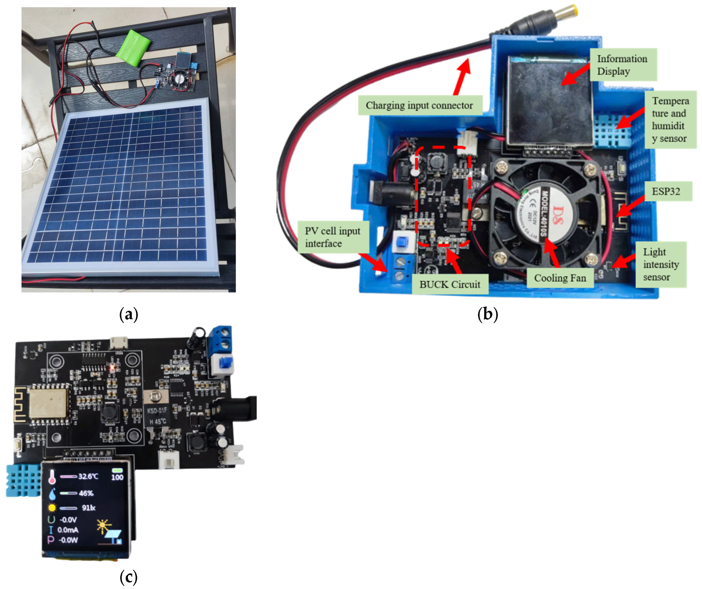
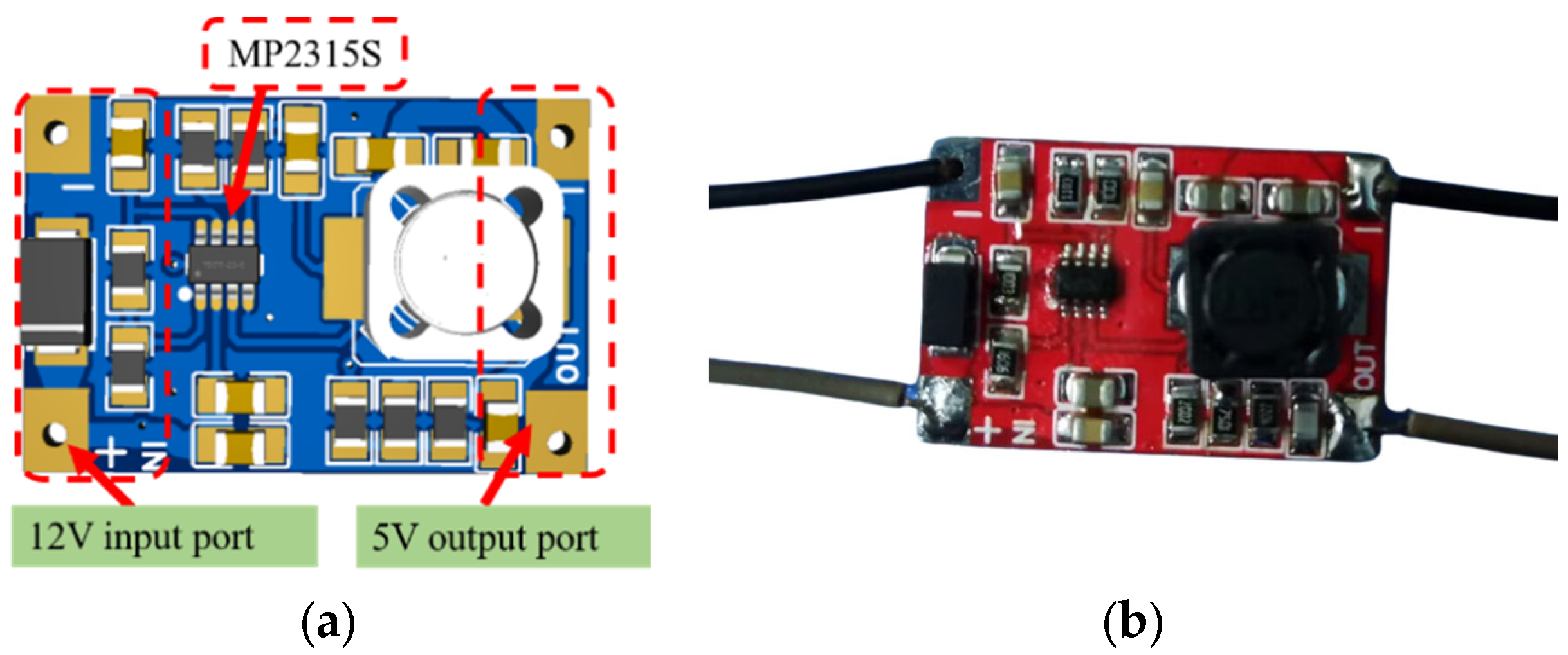
6.1. Hardware Circuit Overall Structure

The information transmission process is as follows: the sensor will collect the information after Kalman filter processing, and then transmit the optimal estimated value to ESP32 microprocessor through the serial port. After a series of regular storage and analysis of the data, the ESP32 carries out MPPT control of the photovoltaic cells and battery power information monitoring. The ESP32 controller can deliver the system work information to the coordinator through MQTT communication technology, and then the coordinator sends it to the upper computer Blinker for remote monitoring through the network terminal nodes and routers. The advantage of this system is that not only does it complete the basic photovoltaic cells MPPT control, but also allows the operator to monitor the working status of the system in real time with the help of IOT communication technology, and the physical MPPT control system designed in this research is shown in Figure 16. When working in hot weather, a 12 V cooling fan is added in combination with a temperature control switch to prevent components from triggering overheating protection.

The hardware circuit part of the MPPT control system studied in this paper contains five main parts: sensor information acquisition, display driver circuit design, ESP32 minimum system circuit design, DC-DC power supply circuit design, and BUCK circuit design.

The sensor information is acquired mainly for the light intensity, output voltage and current, temperature and humidity around the solar panel, calculating the temperature of the PCB through the NTC thermistor, and starting the cooling fan to cool down when the PCB temperature is greater than 45 °C. The information collected by the sensors is processed by the ESP32 microprocessor’s Kalman filter algorithm and sent to the host computer Blinker for remote monitoring via a network communication protocol. The wireless access point and wireless terminal of Wi-Fi network use ESP32 chip launched by Espressif company, which adopts TSMC low-power 40 nm technology and has a complete TCP/IP protocol stack [45]. The communication between the modules of this system is shown in Figure 17.

The DHT11 digital temperature and humidity sensor is used to measure the temperature and humidity data of the environment in which the solar panel is located. The sensor has strong anti-interference capability and is a temperature and humidity composite sensor containing a calibrated digital signal output, which is internally composed of a resistive moisture sensing element and an NTC temperature measuring element with an operating current of less than 2.5 mA, a measuring inaccuracy of 2 °C and a temperature measurement range of −20 to 60 °C, and a humidity measurement range from 20% to 95% with a measurement error of ±5%.

The BH1750 light intensity sensor is used to collect the light intensity received by the solar panel, which consists of a 16-bit AD digital-to-analog converter internally and can accurately measure the light intensity in the range from 0 to 65,535 LX. The INA226 power detection IC is used for photovoltaic cell output voltage and current detection, which can detect the bus voltage range from 0 to 36 V with a measurement error of ±0.1%, and its measurement accuracy can largely avoid the impact of system errors on the MPPT control algorithm. The power module of ESP32 main control circuit uses the MP2315S, which is a high-efficiency synchronous buck rectifier switching converter with built-in power MOSFETs, maximum input voltage of 24 V and maximum output current of 3 A, as well as over-current protection, over-voltage protection, and over-temperature protection. The circuit PCB of the power module of the MPPT control system studied in this paper is shown in Figure 18.

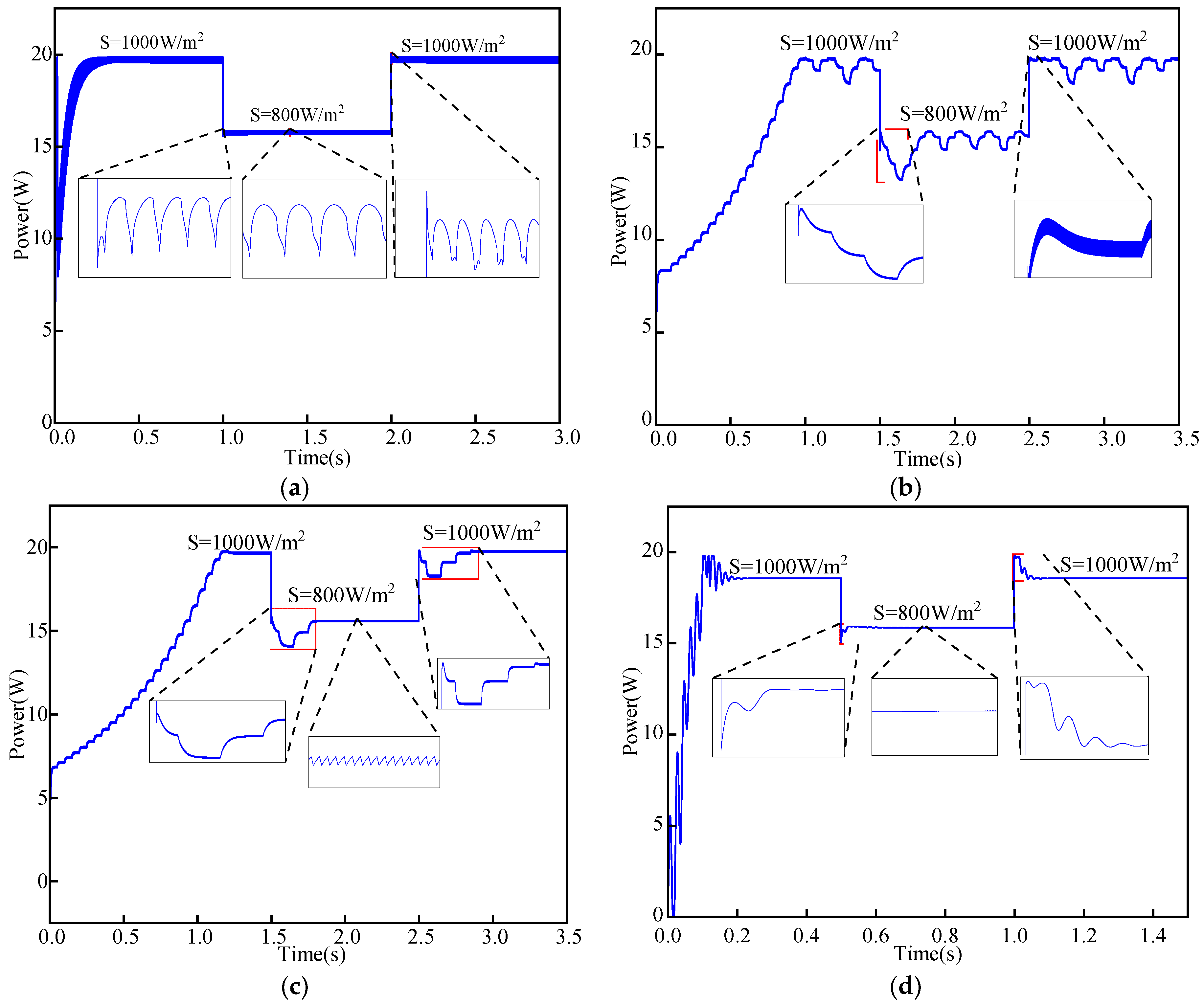
6.2. Analysis of Test Results

The test was conducted in the laboratory with an adjustable light source, setting the initial light intensity to 1000 W/m² and the ambient temperature to 25 °C. The light intensity was set to fluctuate at intervals, as illustrated in Figure 19 for various MPPT control algorithms, to test the way in which photovoltaic cells produced their output when the light intensity changed quickly.

In the whole simulation process, the dramatic change in light intensity is divided into two processes of increasing and decreasing, the dynamic response time and stability of each algorithm are compared in the two cases, and the results of different MPPT control algorithms are shown in

Table 4. Comparison of Dynamic Response Time.

	Response Time
MPPT Algorithms	Start-up time	Light reduction	Light increase
Constant voltage method	0.1	0.005	0.004
Perturbation observation method	1.02	0.25	0.19
Constant step conductance increment method	1.2	0.28	0.35
Improved MPPT algorithms	0.12	0.01	0.06

.

The findings in Table 4 show that when the light intensity increased dramatically, the constant voltage approach responded the quickest, followed by the proportional-integral-derivative incremental conductance method developed in this research. The reason why the MPPT control algorithm designed in this paper has a slightly slower response time than the constant voltage method is that the Kalman filter is used for data pre-processing, which occupies part of the time in this part. In this experimental test, the steady values of light intensity are 800 W/m² and 1000 W/m², and the average output power of different MPPT control algorithms when the light intensity reached the steady state is shown in

Table 5. Comparison of Average Power at Constant Light Intensity.

MPPT Algorithms	800 W/m2	1000 W/m2	Tracking Accuracy
Constant voltage method	15.76	19.69	96.5%
Perturbation observation method	15.35	19.08	86.7%
Constant step conductance increment method	15.59	19.77	97.5%
Improved MPPT algorithms	15.85	19.78	99.6%

.

From the data in Table 5, it can be seen that the theoretical values of the maximum output power of the PV cells are 15.85 W and 19.78 W when the light intensity is 800 W/m² and 1000 W/m². The tracking accuracy of the perturbation observation method is the worst because the process of its maximum power point tracking has been in a fluctuating state. The analysis of the simulation results shows that both MPPT algorithms can achieve monitoring the highest power point, but the tracking speed and tracking accuracy of their algorithms are very different. Among them, the quickest dynamic reaction is provided by the constant voltage approach, but its tracking accuracy is only 96.5%, and as can be seen from Figure 19a, after tracking the maximum power point, its power generated is not constant. The perturbation observation method produces misjudgment when the light intensity changes drastically, which seriously affects the dynamic tracking accuracy, and its simulation tracking accuracy was only 86.7%. For the fixed step incremental conductance method, the perturbation step is proportional to the dynamic response speed and inversely proportional to the steady-state tracking accuracy, and the value of the fixed step has a very strong influence on the tracking effect and is easily caught in the local optimum. In this paper, the newly developed step size incremental conductance approach has very quick dynamic response times in addition to excellent tracking accuracy; meanwhile, it can solve the problems of local optimum under partial shading conditions.

7. Conclusions

Aiming at the problems that the fixed step algorithm and the traditional variable step incremental conductance method are difficult to balance the dynamic response speed and steady-state accuracy due to the step selection, slow start-up speed and local optimum under the condition of sudden change in light intensity, the improved various parameter incremental conductance method presented in this paper is based on the Kalman filter algorithm. By building the corresponding hardware circuit for testing, we can obtain the following conclusions:

(1)

By examining the effect of environmental elements on the output properties of photovoltaic cells, it can be determined that the temperature has little effect and that the short-circuit current and open-circuit voltage of photovoltaic cells both increase with an increase in light intensity.

(2)

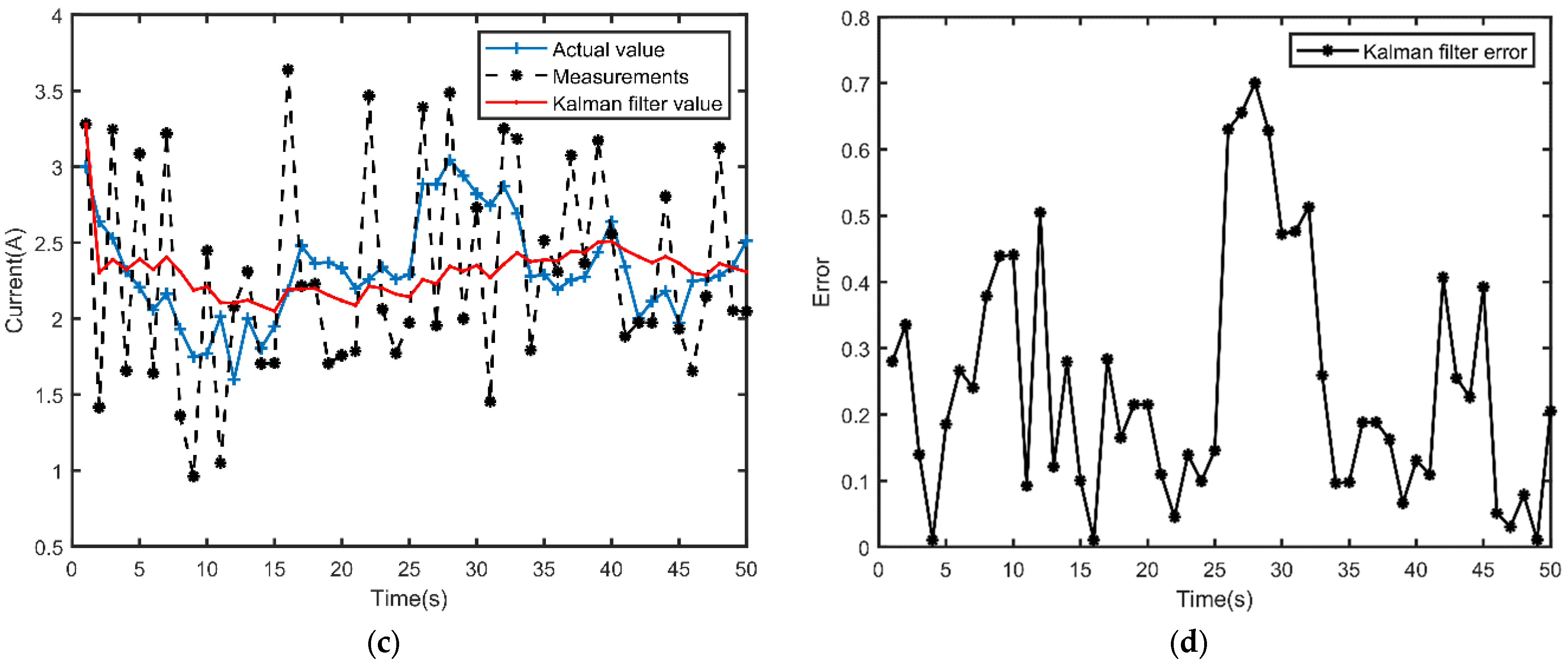
The measurement error of the sensor can be decreased to 32% by utilizing the Kalman filtering technique to pre-process the output voltage and current of the photovoltaic cells. This significantly increases the steady-state accuracy of the MPPT control.

(3)

When Kalman filter parameters were adjusted, it was discovered that the output of the filter is strongly correlated with both the process noise covariance matrix (Q) and the measurement noise covariance matrix (R). When the value of Q increases, the dynamic response of the system becomes faster, but the convergence at stabilization becomes worse. When the value of R increases, the dynamic response of the system slows down, though the convergence stability of the system improves. In the process of parameter adjustment, the values of Q and R cannot be zero at the same time, and the output effect of Kalman filter is only related to the ratio of Q and R.

(4)

In calculating the disturbance step based on (24), there is no cyclic judgment condition, which largely improves the calculation speed of MPPT control. After physical testing, the photovoltaic MPPT control system designed in this paper has a tracking accuracy of 99.6% and low fabrication cost and fastest dynamic response time of 0.01 s in comparison to traditional MPPT control algorithms, which can meet the scenario of small power photovoltaic power generation applications.

(5)

In practical applications, the solar power system designed in this paper can be applied to street lights, unmanned boats and other scenarios that require power supply in the natural environment. The core of the MPPT control algorithm lies in the calculation of the perturbation step. In this paper, a three-stage perturbation step calculation method is proposed and verified, and the parameters of the perturbation step can be adjusted according to needs to meet particular design applications.

References

1. Liao, C.Y.; Subroto, R.K.; Millah, I.S.; Lian, K.L.; Huang, W.T. An Improved Bat Algorithm for More Efficient and Faster Maximum Power Point Tracking for a Photovoltaic System Under Partial Shading Conditions. IEEE Access 2020, 8, 96378–96390. [Google Scholar] [CrossRef]
2. Zinatloo-Ajabshir, S.; Morassaei, M.S.; Amiri, O.; Salavati-Niasari, M. Green synthesis of dysprosium stannate nanoparticles using Ficus carica extract as photocatalyst for the degradation of organic pollutants under visible irradiation. Ceram. Int. 2020, 46, 6095–6107. [Google Scholar] [CrossRef]
3. Liu, B.; Sharma, M.; Yu, J.; Wang, L.; Shendre, S.; Sharma, A.; Izmir, M.; Delikanli, S.; Altintas, Y.; Dang, C.; et al. Management of electroluminescence from silver-doped colloidal quantum well light-emitting diodes. Cell Rep. Phys. Sci. 2022, 3, 100860. [Google Scholar] [CrossRef]
4. Liu, K.C. Review on reliability assessment of smart distribution networks considering distributed renewable energy and energy storage. Electr. Meas. Instrum. 2021, 58, 1–11. [Google Scholar]
5. Zhou, D.B. Maximum Power Point Tracking Strategy Based on Modified Variable Step-Size Incremental Conductance Algorithm. Power Syst. Technol. 2015, 39, 1491–1498. [Google Scholar]
6. Cai, L. Test System for Power Generation Characteristics of Photovoltaic Modules Based on Real-Time Parameters. Laser Optoelectron. Prog. 2017, 54, 395–401. [Google Scholar]
7. Xiao, Y.; Li, S.; Xu, M.; Feng, R. Research on the economy of implementing the MPPT for wind-solar hybrid power generation system: A review. In Proceedings of the 41st Chinese Control Conference, Hefei, China, 25–27 July 2022; pp. 2–7. [Google Scholar]
8. Troudi, F.; Jouini, H.; Mami, A.; Ben Khedher, N.; Aich, W.; Boudjemline, A.; Boujelbene, M. Comparative Assessment between Five Control Techniques to Optimize the Maximum Power Point Tracking Procedure for PV Systems. Mathematics 2022, 10, 1080. [Google Scholar] [CrossRef]
9. Owusu-Nyarko, I.; Elgenedy, M.A.; Abdelsalam, I.; Ahmed, K.H. Modified Variable Step-Size Incremental Conductance MPPT Technique for Photovoltaic Systems. Electronics 2021, 10, 2331. [Google Scholar] [CrossRef]
10. Zhang, D. Research on photovoltaic maximum power point tracking strategy based on improved conductance increment method. J. Sol. Energy 2022, 43, 82–90. [Google Scholar]
11. Hannachi, M.; Elbeji, O.; Benhamed, M.; Sbita, L. Comparative study of four MPPT for a wind power system. Wind. Eng. 2021, 45, 1613–1622. [Google Scholar] [CrossRef]
12. Kumar, N.; Hussain, I.; Singh, B.; Panigrahi, B.K. Self-Adaptive Incremental Conductance Algorithm for Swift and Ripple-Free Maximum Power Harvesting from PV Array. IEEE Trans. Ind. Inform. 2018, 14, 2031–2041. [Google Scholar] [CrossRef]
13. Li, X.; Xu, J. Maximum power point tracking control for grid-connected photovoltaic power generation system. Comput. Simul. 2019, 36, 117–121. [Google Scholar]
14. Xu, J.; Wang, H. The hybrid control Maximum Power Point Tracking (MPPT) strategy based on incremental conductance method and improved particle swarm optimization algorithm. Renew. Energy Resour. 2019, 37, 824–831. [Google Scholar]
15. Sheikh Ahmadi, S.H.; Karami, M.; Gholami, M.; Mirzaei, R. Improving MPPT Performance in PV Systems Based on Integrating the Incremental Conductance and Particle Swarm Optimization Methods. Iran. Sci. Technol. Trans. Electr. Eng. 2022, 46, 27–39. [Google Scholar] [CrossRef]
16. Mi, D.; Hu, J.; Jian, Y. An improved slime mould algorithm based MPPT strategy for multi-peak photovoltaic system. Control Theory Appl. 2022, 39, 1–9. [Google Scholar]
17. Ali, Z.M.; Alquthami, T.; Alkhalaf, S.; Norouzi, H.; Dadfar, S.; Suzuki, K. Novel hybrid improved bat algorithm and fuzzy system based MPPT for photovoltaic under variable atmospheric conditions. Sustain. Energy Technol. Assess. 2022, 52, 102156–102179. [Google Scholar] [CrossRef]
18. Liu, C.; Sun, Y. Tracking Strategy of Maximum Power Point Based on Three-Stage Variable Step-Size Incremental Conductance Algorithm. Laser Optoelectron. Prog. 2018, 55, 420–426. [Google Scholar]
19. Cui, Z. Research progress and prospects of photocatalytic devices with perovskite ferroelectric semiconductors. J. Phys. 2020, 69, 51–83. [Google Scholar] [CrossRef]
20. Sabaripandiyan, D.; Sait, H.H.; Aarthi, G. A Novel Hybrid MPPT Control Strategy for Isolated Solar PV Power System. Intell. Autom. Soft Comput. 2022, 32, 1055–1070. [Google Scholar] [CrossRef]
21. Senthilkumar, S.; Mohan, V.; Mangaiyarkarasi, S.P.; Karthikeyan, M. Analysis of Single-Diode PV Model and Optimized MPPT Model for Different Environmental Conditions. Int. Trans. Electr. Energy Syst. 2022, 2022, 4980843. [Google Scholar] [CrossRef]
22. Annapoorani, S.; Jayaparvathy, R. Modified Seagull Optimization Algorithm based MPPT for augmented performance of Photovoltaic solar energy systems. Automatika 2022, 63, 286601. [Google Scholar]
23. Sarwar, S.; Hafeez, M.A.; Javed, M.Y.; Asghar, A.B.; Ejsmont, K. A Horse Herd Optimization Algorithm (HOA)-Based MPPT Technique under Partial and Complex Partial Shading Conditions. Energies 2022, 15, 1880. [Google Scholar] [CrossRef]
24. Zhang, J. Research on MPPT Algorithm of Photovoltaic Power Generation System Based on LabVIEW. J. Taiyuan Univ. Technol. 2018, 49, 477–482. [Google Scholar]
25. Rui, Z.; Bo, Y.; Nuo, C. Arithmetic optimization algorithm based MPPT technique for centralized TEG systems under different temperature gradients. Energy Rep. 2022, 8, 2424–2433. [Google Scholar]
26. Cao, D. Improved Ant Colony Optimization Algorithm for Multi-object Routing in Energy Harvesting Wireless Sensor Networks. J. Chin. Comput. Syst. 2021, 42, 1115–1120. [Google Scholar]
27. Boghdady, T.A.; Kotb, Y.E.; Aljumah, A.; Sayed, M.M. Comparative Study of Optimal PV Array Configurations and MPPT under Partial Shading with Fast Dynamical Change of Hybrid Load. Sustainability 2022, 14, 2937. [Google Scholar] [CrossRef]
28. Liang, C. Photovoltaic multi peak MPPT control based on Improved Particle Swarm Optimization. In Proceedings of the 2022 34th Chinese Control and Decision Conference (CCDC), Hefei, China, 21–23 May 2022; pp. 389–394. [Google Scholar]
29. Hussaian, B.C.; Matcha, M. A new design of transformerless, non-isolated, high step-up DC-DC converter with hybrid fuzzy logic MPPT controller. Int. J. Circuit Theory Appl. 2021, 50, 302–321. [Google Scholar]
30. Guo, C. Fuzzy control based variable step conductance increment method for maximum power point tracking strategy. Mod. Electron. Tech. 2022, 45, 145–151. [Google Scholar]
31. Pires, V.F.; Cordeiro, A.; Foito, D.; Silva, J.F. Control transition mode from voltage control to MPPT for PV generators in isolated DC microgrids. Int. J. Electr. Power Energy Syst. 2022, 137, 107876–107895. [Google Scholar] [CrossRef]
32. Touhami, G.; Sliman, L.; Zohra, A.F.; Abdelkader, H.; Khalil, D. Extraction of Maximum Power of Organic Photovoltaic Generator Using MPPT Technique. Appl. Mech. Mater. 2022, 905, 1–6. [Google Scholar] [CrossRef]
33. Villegas-Mier, C.G.; Rodriguez-Resendiz, J.; Álvarez-Alvarado, J.M.; Rodriguez-Resendiz, H.; Herrera-Navarro, A.M.; Rodríguez-Abreo, O. Artificial Neural Networks in MPPT Algorithms for Optimization of Photovoltaic Power Systems: A Review. Micromachines 2021, 12, 1260. [Google Scholar] [CrossRef] [PubMed]
34. Pradhan, C.; Senapati, M.K.; Ntiakoh, N.K.; Calay, R.K. Roach Infestation Optimization MPPT Algorithm for Solar Photovoltaic System. Electronics 2022, 11, 927. [Google Scholar] [CrossRef]
35. Sousa, S.M.; Gusman, L.S.; Lopes TA, S.; Pereira, H.A.; Callegari, J.M.S. MPPT algorithm in single loop current-mode control applied to dc–dc converters with input current source characteristics. Int. J. Electr. Power Energy Syst. 2022, 138, 107909–107927. [Google Scholar] [CrossRef]
36. Awan, M.M.A.; Javed, M.Y.; Asghar, A.B.; Ejsmont, K. Performance Optimization of a Ten Check MPPT Algorithm for an Off-Grid Solar Photovoltaic System. Energies 2022, 15, 2104. [Google Scholar] [CrossRef]
37. Li, S. Research on Internet of Things Acquisition System in Greenhouse Based on the Improved Kalman Data Fusion Algorithm. Chin. J. Sens. Actuators 2022, 35, 558–564. [Google Scholar]
38. Dong, Z. A new state monitoring method for IoT sensor based on Kalman filter algorithm. Int. J. Auton. Adapt. Commun. Syst. 2021, 13, 448–463. [Google Scholar] [CrossRef]
39. Wang, E.; Xiao, L.; Han, X.; Tan, B.; Luo, L. Design of an Agile Training System Based on Wireless Mesh Network. IEEE Access 2022, 529, 84302–84316. [Google Scholar] [CrossRef]
40. Tan, B.; Wang, E.; Cao, K.; Xiao, L.; Luo, L. Study and Design of Distributed Badminton Agility Training and Test System. Appl. Sci. 2023, 13, 1113. [Google Scholar] [CrossRef]
41. Zhang, Z. Design of home intelligent elderly care monitoring system. Mod. Electron. Tech. 2022, 45, 171–176. [Google Scholar]
42. Peng, D.C. Basic Principle and Application of Kalman Filter. Softw. Guide 2009, 8, 32–34. [Google Scholar]
43. Osman, H.H.; Ismail, I.A.; Morsy, E.; Hawidi, H.M. Implementing the Kalman Filter Algorithm in Parallel Form: Denoising Sound Wave as a Case Study. Recent Adv. Comput. Sci. Commun. 2021, 14, 2828–2835. [Google Scholar] [CrossRef]
44. Liu, F. Kalman filter based method for processing small noisy sample data. J. Shanghai Univ. (Nat. Sci. Ed.) 2022, 28, 427–439. [Google Scholar]
45. Yuan, S.; Shengyuan, Y.; Yanxia, S. A Wind Speed Prediction Model Based on ARIMA and Improved Kalman Filter Algorithm. J. Phys. Conf. Ser. 2020, 1650, 032095. [Google Scholar] [CrossRef]
46. Tan, B.; You, W.; Tian, S.; Xiao, T.; Wang, M.; Zheng, B.; Luo, L. Soil Nitrogen Detection Based on Random Forest Algorithm and Near-Infrared Spectroscopy. Sensors 2022, 22, 8013. [Google Scholar] [CrossRef] [PubMed]
47. Tan, B.; You, W.; Huang, C.; Xiao, T.; Tian, S.; Luo, L.; Xiong, N. An Intelligent Near-Infrared Diffuse Reflectance Spectroscopy Scheme for the Non-Destructive Testing of the Sugar Content in Cherry Tomato Fruit. Electronics 2022, 11, 3504. [Google Scholar] [CrossRef]
48. Cai, Z.D.; Xu, J.Y.; Sun, X.Y.; Di Quan, L. SOC Estimation of Modular Lithium Battery Pack Based on Adaptive Kalman Filter Algorithm. J. Phys. Conf. Ser. 2019, 1345, 1. [Google Scholar] [CrossRef]
49. You, D.; Liu, P.; Shang, W.; Zhang, Y.; Kang, Y.; Xiong, J. An Improved Unscented Kalman Filter Algorithm for Radar Azimuth Mutation. Int. J. Aerosp. Eng. 2020, 2020, 8863286. [Google Scholar] [CrossRef]
50. Li, S.; Zhang, M.; Ji, Y.; Zhang, Z.; Cao, R.; Chen, B.; Li, H.; Yin, Y. Agricultural machinery GNSS/IMU-integrated navigation based on fuzzy adaptive finite impulse response Kalman filtering algorithm. Comput. Electron. Agric. 2021, 191, 106524–106543. [Google Scholar] [CrossRef]
Figure 1. Photovoltaic effect principle.
Energies 16 01299 g001
Figure 2. Photovoltaic cell equivalent circuit diagram.
Energies 16 01299 g002
Figure 3. Photovoltaic cell output characteristics curve.
Energies 16 01299 g003
Figure 4. Effect of temperature on the output characteristics of the photovoltaic cells. (a) I-U. (b) P-U.
Energies 16 01299 g004
Figure 5. Effect of light intensity on the output characteristics of the photovoltaic cells. (a) I-U. (b) P-U.
Energies 16 01299 g005
Figure 6. P-U characteristic of photovoltaic array under PSC.
Energies 16 01299 g006
Figure 7. Photovoltaic cell linear equivalent circuit.
Energies 16 01299 g007
Figure 8. Photovoltaic system structure diagram.
Energies 16 01299 g008
Figure 9. The features of dP/dU variation of P-U characteristics of the photovoltaic cells.
Energies 16 01299 g009
Figure 10. General block diagram of MPPT control system.
Energies 16 01299 g010
Figure 11. Kalman filter algorithm application diagram.
Energies 16 01299 g011
Figure 12. (a) Results of Kalman filtering algorithm for output voltage. (b) Error between the voltage filtered value and the real value. (c) Results of Kalman filtering algorithm for output current. (d) Error between the current filtered value and the real value.
Energies 16 01299 g012aEnergies 16 01299 g012b
Figure 13. Schematic diagram of three-stage variable step conductance increment method.
Energies 16 01299 g013
Figure 14. Improving variable step MPPT control algorithm process.
Energies 16 01299 g014
Figure 15. Improved Simulation Model of Three-Stage Variable Step Incremental Conductance Method.
Energies 16 01299 g015
Figure 16. (a) Outdoor practical working test chart. (b) Manufactured PCB for the DC–DC converter optimally designed for the photovoltaic application. (c) Main control board details.
Energies 16 01299 g016
Figure 17. Communication relations of each module.
Energies 16 01299 g017
Figure 18. (a) DC-DC controller, PCB layout. (b) DC-DC controller, physical picture.
Energies 16 01299 g018
Figure 19. (a) Constant voltage method. (b) Perturbation observation method. (c) Constant step conductance increment method. (d) Three-stage variable step conductance increment method based on Kalman filter.
Energies 16 01299 g019