Abstract
A new explicit sequentially coupled technique for chemo-thermo-poromechanical problems in shale formations is developed. Simultaneously solving the flow and geomechanics equations in a single step is computationally expensive with consequent limitations on the computations involving well or reservoir-scale geometries. The newly developed solution sequence involves solving the temperature field within the porous system. This is followed by the computation of the chemical activity constrained by the previously computed temperature field. The pore pressure is then computed by coupling the pore thermal and chemical effects but without consideration of the volumetric strains. The geomechanical effect of the volumetric strain, stress tensors, and associated displacement vectors on the pore fluid is subsequently computed explicitly in a single-step post-processing operation. By increasing the borehole pressure to 20 MPa, it is observed that the rock displacement and velocities concurrently increase by 50%. However, increasing the wellbore temperature and chemical activities shows only a slight effect on the rock and pore fluid. In the chemo-thermo-poroelasticity steady-state simulation, the maximum displacements recorded in the and are 0.00633 m and 0.0035 m, respectively, for 2D and 0.21 for the 3D simulation. In the transient simulation, the displacement values are observed to increase gradually over time with a corresponding decrease in the maximum pore-fluid velocity. A comparison of this work and the partial two-way coupling scheme in a commercial simulator for the 2D test cases was carried out. The maximum differences between the computed temperatures, displacement values, and fluid velocities are , , and , respectively. The analysed results, therefore, indicate that this technique is comparatively accurate and more computationally efficient than running a full or partial two-way coupling scheme.
1. Introduction
The numerical simulation of flow in shale gas and oil formations is challenging from a static geological modelling and dynamic simulation point of view. Advances in horizontal drilling and hydraulic fracturing have transformed the characterisation and modelling of these flow processes. However, the simulation of the flow and transport of gas or oil in shale formations is complex and usually relies on coupling models capable of capturing, for example, wellbore stability, hydraulic fracturing, compaction drive, subsidence, and thermal fracturing [1]. In these situations, the mechanical response of the rock depends on the pore-fluid flow and inherent changes that occur within the pore volume. This coupled response is usually modelled using Biot’s poroelastic theory [2,3,4,5,6,7,8]. Surprisingly, many reservoir simulation programs used in the petroleum industry adopt a technique whereby geomechanics is not coupled to fluid flow but evaluated independently based on rock and thermal compressibility. Reservoir geomechanics problems combine the hydraulics and the thermal and chemical flow effects on rock mechanics in a coupled manner. Thus, the solution method implemented for such problems should involve solving the governing differential equations using a coupled solution technique [9]. By introducing the poroelasticity concept, it has been shown that it is indeed possible to develop a coupled model that solves the fluid flow within the porous medium, as well as the geomechanical problem [2,3,9,10]. In this case, the fluid flow behaviour is described using Darcy’s law and the geomechanics behaviour by a stress–strain relationship and the stress equilibrium equation. Chemical and thermal effects have also been accounted for using the conservation of energy equation [7,11,12]. In their work, [10] developed a fully coupled fluid compositional geomechanical reservoir simulator to model the injection of water and gas for the protection of a parent well. The developed model, however, considers the isothermal condition and does not include the thermal diffusion effect in the coupled equation.
Ref. [13] investigated the effects of heterogeneity and thermal perturbation uncertainties in the estimation of in situ stresses. They used heuristic models including heterogeneity to investigate potential errors in the estimation of far-field stresses associated with the generalisation of Kirsch’s equations and plausible temperature perturbations. Finite element analysis (FEA) has recently become more popular in geomechanics and reservoir engineering (e.g., [14,15,16]. This is due to the fact that FEA can provide a detailed understanding of the subsurface geological and mechanical behaviour. However, simultaneously solving the flow and geomechanics equations in a single solution can be laborious and computationally expensive. It is in this vein that different coupling schemes were developed when dealing with reservoir geomechanics [17]. Generally, the coupling schemes are classified as either full or partial (iterative) coupling. The partial coupling scheme is further subdivided into one-way and two-way partial couplings. In the case of one-way or explicit coupling, the flow variable, which is usually the pore pressure, is computed separately and used as an input variable to update the stress field. This is achieved via the Biot poroelastic coupling term at each time step. However, the computed stress field does not affect the pore pressure [9]. It takes into account the dynamic effects of fluid flow patterns and behaviour on the geomechanical behaviour of the coupled rock–fluid system but there is no feedback in the reverse direction. In a one-way (or explicit) coupling method, geomechanics computation is carried out entirely as a post-processing operation, making it quite adaptable and fast. An appropriate technique must, therefore, be used in quantifying the error limit and degree of accuracy of any adopted algorithm.
In a two-way partial coupling scheme, the flow variable is computed at each time step and then used to update the stress field. The computed displacements are then used to compute the new pressure at the next time step until solution convergence is achieved. In this method, the geomechanical response of the rock through the pore volume changes the feeds back into the fluid flow model [17]. In the case of the full coupling approach, the flow and geomechanics are computed simultaneously from known initial and boundary conditions in an implicit manner. As previously mentioned, this fully coupled method can be very complicated and requires a robust solution technique alongside a fast and efficient solver. The need for such solvers is due to the usually large matrices that are realised when solving the partial differential equations (from the governing equations) using numerical techniques such as the finite-element method [9]. Furthermore, it is usually practically impossible to use this approach in modelling chemo-thermo-poroelasticity flow in realistic well or reservoir models consisting of tens or hundreds of thousands of geometric meshes.
In describing the permeability of shale formations, [18] studied how the distribution of a fracture aperture affects gas apparent permeability. Ref. [19] used micro- and nano-computed tomography images of shale rock samples obtained from Mancos, Marcellus, and Eagle Ford formations to characterise and quantify the permeability, porosity, and tortuosity, as well as the heterogeneity factor. However, the effect of chemo-thermo-poroelasticity on these properties was not investigated. Refs. [20,21] proposed a local model order reduction technique that was applied to a hydraulic fracturing process described by a nonlinear parabolic PDE system with a time-dependent spatial domain. This model was shown to be more accurate and computationally efficient in approximating the original nonlinear system with fewer eigenfunctions compared to the model order reduction technique with temporally global eigenfunctions.
It is understood that shale formations are susceptible to moisture absorption, with consequent swelling and weakening leading to wellbore instability problems. This is due to their structure and mineralogical content. Various studies have shown that drilling through shale formations is a challenge yet to be surmounted. The development of mathematical models that will not only predict optimum drilling conditions but also the most appropriate drilling fluid formulations have been proffered as a solution to the problem. This has led to the development of various types of wellbore instability models. These studies have been conducted over the years from a geomechanics point of view. This was achieved by analysing how formation in-situ stresses affect the mechanical rock properties in relation to stress redistribution around the wellbore during drilling processes. However, in the case of shale formations, this approach was found to be insufficient and the studies were extended to investigate the chemical interactions between aqueous fluids and shale formations that result in swelling and its consequent drilling problems.
Therefore, developing a solution approach that will embrace the accuracy of a full coupling scheme involving the chemical, thermal, and poroelastic properties of the rock-fluid interaction will be beneficial. Further, consideration for the speed and efficiency of a partially coupled scheme will be extremely advantageous. Most of the existing models solve the problems of the coupled models by simultaneously solving the flow and geomechanics equations in a single step. This is computationally expensive with consequent limitations on the computation involving well or reservoir-scale geometries. At these scales, physical models are usually represented by millions of finite elements. Some fully coupled models usually exclude chemical or thermal effects. In most cases, the equations are solved on simple geometries due to the high computational resource requirements. This research is, therefore, aimed at proffering a solution to this challenge.
A new solution methodology for chemo-thermo-poroelasticity is hereby developed by implementing an explicitly coupled sequential algorithm coded in a complex system modelling platform (CSMP++). CSMP++ is a C++-based object-oriented application platform. This methodology is applied successfully to model wellbore stability in a computationally efficient manner. This is aimed at solving problems where computational efficiency, which may be lacking in the fully coupled model’s computation, is desirable. The governing equations describe a non-isothermal physico-chemical problem involving solid matrix deformations, fluid and ionic flow through the pore spaces, and heat flux through the solid porous media and pore fluid.
2. Governing Equations
The mathematical model applied in this study was developed based on the study of poro-mechanics (i.e., the mechanical response of fluid-saturated porous media) and non-equilibrium thermodynamics. The governing equations in this study describe a non-isothermal physico-chemical problem involving solid matrix deformations, fluid and ionic flow through the pore spaces, and heat flux through the solid porous media and pore fluid. These equations are derived based on the constitutive relations between the solid matrix and pore space, conduction laws covering the transport of solvent and solutes of a multi-component system, and heat diffusion, alongside the laws of conservation of momentum, mass, and energy.
The development and formulation of the governing equations have been presented in a previous work [22]. The coupled poro-chemo-thermoelastic model considering multiple solutes is highlighted by considering the following:
The Navier-type equation
The solvent diffusion equation
The solute diffusion equation
The thermal diffusion equation
where u, is the rock displacement, p is the pore pressure, is the chemical activity, T is the temperature, K is the bulk modulus of the rock, G is the shear modulus of the rock, is the Biot’s coefficient, X and are the chemical coupling terms, and are the thermal coupling terms, is the Skempton’s coefficient, k is the hydraulic conductivity, L is the membrane efficiency coefficient, is the porosity, is the pore-fluid density, is the solute diffusion coefficient, is the thermal diffusion coefficient, Q is the thermal diffusivity, and for conditions of plane strain (or two-dimensional problems) or for problems considered in a three- dimensional state of strain. Other constitutive relations include
and .
The Navier-type equation and the solute, solvent, and heat diffusion equations constitute a set of field equations that can be solved simultaneously subject to initial and boundary conditions. These equations present a fully coupled chemo-thermo-poroelastic model considering multi-component drilling and pore-fluid compositions. In the following, the use of the finite-element method for the solution of these equations is presented. This model describes the physio-chemical interactions between drilling fluids and reactive rock formations and can be used for predicting the pore pressure p; formation temperature T; chemical activities ; and, subsequently, wellbore stresses for known drilling fluid formulations when interacting with reservoir rock, e.g., shale. It can be applied as a tool for drilling fluid optimisation and potentially in conjunction with an appropriate rock failure criterion for predicting critical mud weights.
2.1. Finite-Element Discretisation of the Governing Equations
The Bubnov–Galerkin finite-element method of numerical analysis has been applied to solve complex numerical problems over structurally complex geological models. The set of field governing equations developed in this study are solved using a finite-element approach, with the equations discretised in the spatial domain using a Bubnov–Galerkin technique [23,24] and then temporally using backward Euler time stepping due to its unconditional stability [25].
In the standard Galerkin finite-element approximation, a basis/shape function is defined on each finite-element node in a piecewise manner. This is defined such that on a particular node and on the neighbouring nodes. The local variable is, therefore, approximated as , which can also be expressed as [26].
2.1.1. Fully Coupled Matrix Formulation
The fully coupled model is based on the Galerkin finite-element discretisation method and the following approximations:
where, , , , and are the shape functions representing the rock displacement, pore pressure, chemical activity, and temperature, respectively. , , , are the vectors of the nodal values of the velocity components, pressure, chemical activity, and temperature, respectively.
The weak form of the geomechanics equation, Equation (1), is obtained by introducing the finite-element approximations as follows:
where, D is the linear elasticity matrix, t is the traction, b is the body force, F is the matrix of the externally applied loads on the system, and B is the strain-displacement relation matrix. The matrices involved in the geomechanics problem can be rewritten from Equation (10) as
where, K, C, S, and Z are defined using the horizontal curly braces in Equation (10). Similarly, the weak form of the fluid flow transport equation is obtained as follows:
which can similarly be rewritten as
where, F, G, H, I, and J are defined using the horizontal curly braces in Equation (12).
The weak form of the chemical activity diffusion equation is derived as follows:
which is rewritten as
where, M, E, and X are defined using the horizontal curly braces in Equation (14). Finally, the weak form of the temperature diffusion equation is written as
where, V and W are defined by the horizontal curly braces underlying the expressions in Equation (15). The definitions of the matrices that form the numerical integrals resulting from the partial differential equations are shown in the Appendix. These are also referred to as PDE operators. By applying the explicit Euler formulation, the pore-pressure, chemical activity, and thermal diffusion Equations (12), (14), and (16) can be rewritten as
These sets of discretised equations are then rearranged and assembled in their fully coupled forms in a matrix equation as
This matrix equation can simply be expressed as a set of linear algebraic equations and solved simultaneously in the fully coupled approach. The finite-element formulation is implemented in our in-house numerical computation platform (CSMP++), which is a C++-based application platform as discussed later. The solution is compared with that obtained using a commercial software package (COMSOL) and other published data.
2.1.2. CSMP++ Explicit Sequential Coupled Solution Approach
The fully coupled formulation described above is implemented in CSMP++ using an explicit sequentially coupled solution approach. In this approach, the temperature diffusion equation, Equation (20), is first solved to obtain a temperature field. This is then followed by the computation of the chemical activity using Equation (19) using the temperature field solution of the temperature diffusion equation as input. The flow equation is then solved for the pore pressure by first decoupling the displacement field, i.e., in Equation (18). This is based on the assumption that initially, volumetric strains on the pore space due to geomechanical effects are negligible and the coupling between the geomechanical and flow equations can be achieved explicitly by assuming . The resultant flow equation from (18) is the usual reservoir flow simulation equation expressed in its matrix form as
The displacement field is then subsequently obtained from the geomechanical response, Equation (18), by imposing the already calculated pressure, temperature, and chemical activity as the external boundary conditions (e.g., [27]) at every time step as follows:
This is the basis for the explicit sequential coupling technique developed in this work. The feedback effects of geomechanics on the fluid flow can be incorporated by implementing the reservoir porosity update equation that incorporates the volumetric, thermal, and chemical activity-imposed strain. Here, the reservoir porosity is updated at every time step. This is referred to as a two-way partial coupling scheme and is not implemented in the current work.
2.1.3. Finite-Element Modelling for the Explicit Sequential Coupling Method
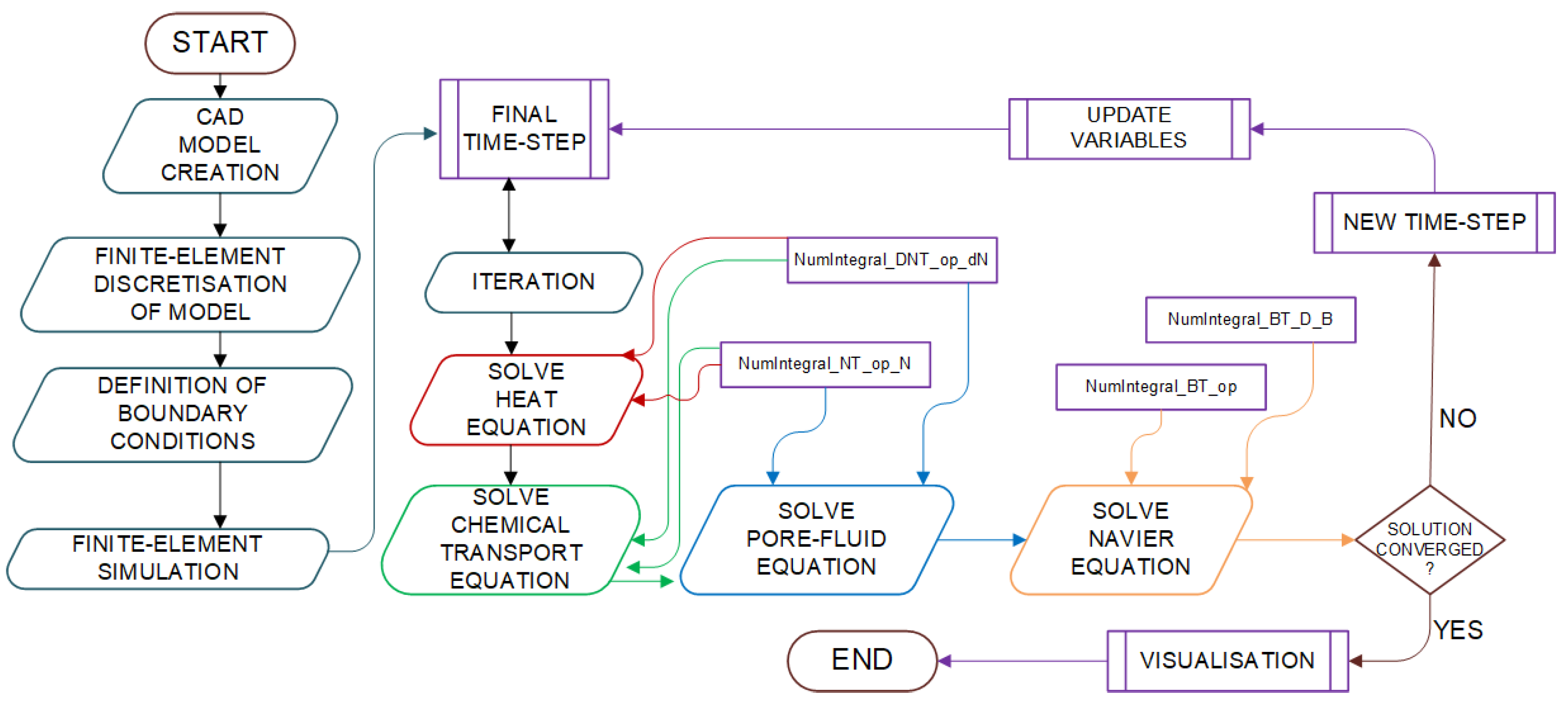
The governing equations presented in Section 2.1.2 can only be solved using numerical methods. We used the finite-element method in this study to discretise the governing equations. Finite-element numerical analysis has previously been applied to solve complex fluid flow in hydrocarbon reservoirs with great success [24,25]. The workflow for a numerical study begins with a description of the computation geometry using a computer-aided design ( CAD) package. The generated system of equations is then solved on the discretised geometry.
In the implementation of the CSMP++ finite-element model, a geometric model is constructed in CAD and meshed using discrete finite elements. The finite-element mesh was imported into CSMP++, where objects representative of the physical entities in the models called supergroups were formed. Initial and boundary conditions are assigned and variable coefficients are computed using the interrelations subclass. Partial differential equations (PDEs) in integral forms arising from the FEM are assembled using numerical PDE operator classes . The computed values of the displacement and pore-fluid velocity are output to VTK for visualisation.
2.1.4. Implementation of the Solution Approach in CSMP++
The set of partial differential equations, Equations (17)–(20), are implemented in CSMP++ and solved for the representative geometric models (see Section 2.1.5). CSMP++ is a C++-based finite-element application programme interface employed to formulate C++ code for solving complex geological problems. CSMP++ is interfaced with the Algebraic Multigrid Solver for Systems (SAMG) for the solution of matrices assembled as linear algebraic equations. The weak forms of the partial differential equations are inserted into the algorithm objects to be computed by the solver using CSMP++ object forms called pde operators (see Table A1). Point-dependent properties such as nodal velocities are processed using objects called visitors [28]. Low-level computations are conducted using CSMP++ objects called interrelations.
In this work, ten interrelation subclasses were developed and coded in the CSMP++ platform for the computation of the coefficient variables highlighted in Table A2. The interrelations were called into the algorithm while carrying out the finite-element computations. Appendix A.4 shows a sample of the C++ code written for the computation of chemical coupling coefficient one.
The workflow begins by generating the computation domain from the mesh followed by declaring the material properties and then defining the initial, essential, and boundary conditions and the coefficients of the partial differential equations (PDEs). The discrete forms of the governing equations are then assembled in matrix form and solved using the SAMG solver [29].
A summary of the workflow of the CSMP++ FEM modelling solution strategy developed in the current work is shown in Figure 1. The solution workflow represents the explicit sequential coupling approach developed in this work. The results from CSMP++ are then compared with those obtained using COMSOL Multiphysics—a commercial simulator.
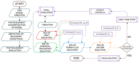
Figure 1.
CSMP++ FEM modelling solution strategy developed in this work.
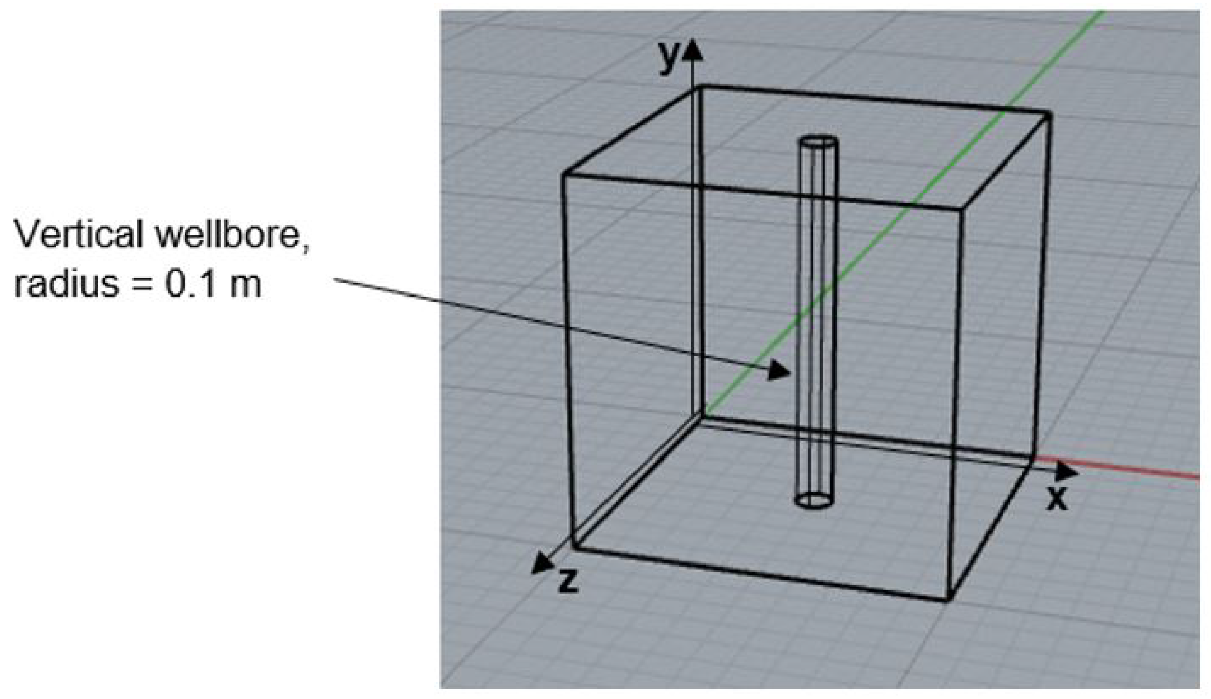
2.1.5. Description of Models and Wellbore Geometry in CSMP++
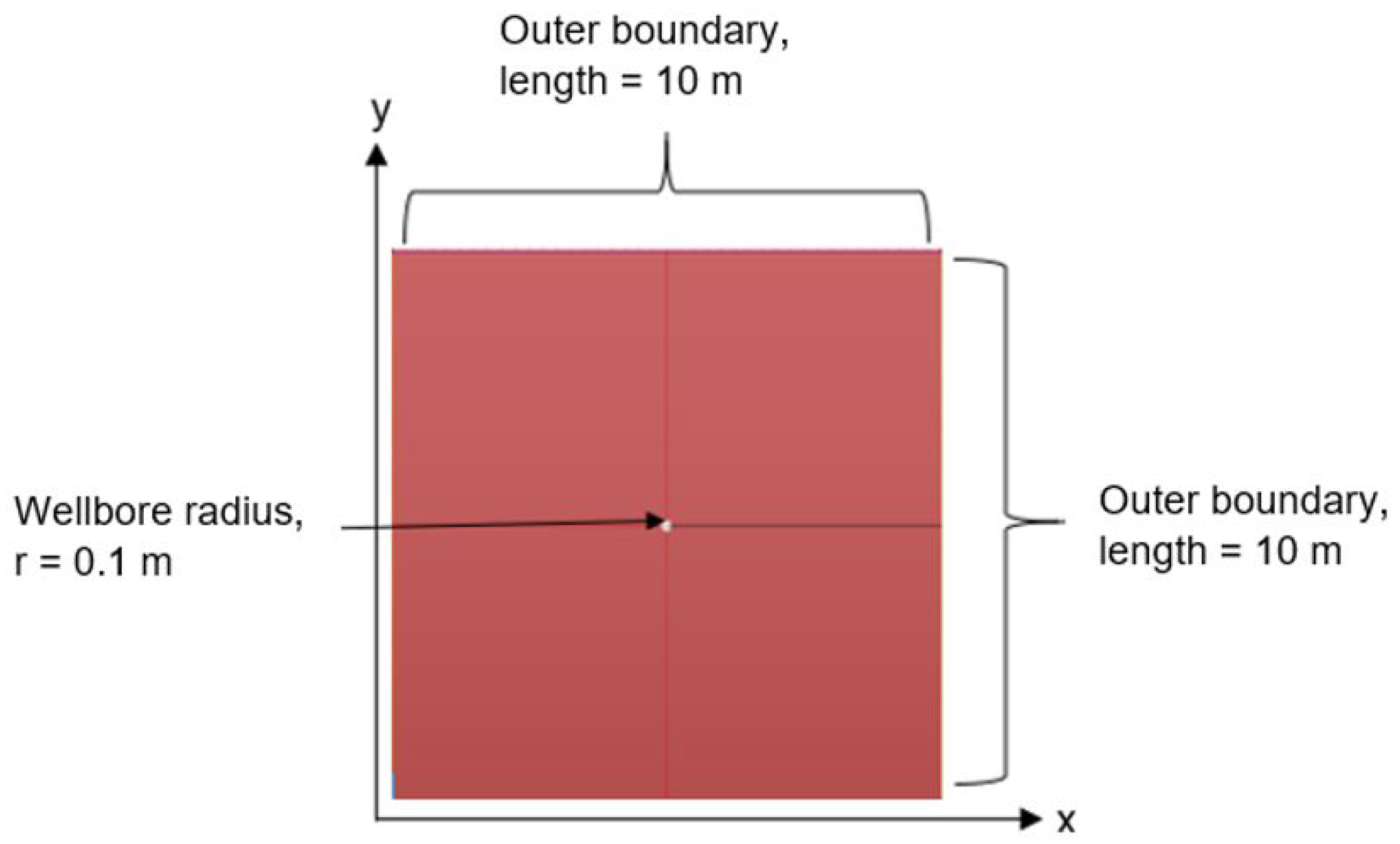
In this work, three geometric models were developed in a computer-aided design (CAD) software package using non-uniform rational B-splines (NURBS). The geometric models consist of two two-dimensional (2D) models and one three-dimensional (3D) model. The first 2D model, a m rectangular model, was used for numerical verification. The second 2D model, a m square model with a centrally placed circular wellbore with a diameter of m, is a representation of a wellbore in a reservoir. The third model is a three-dimensional m model with a borehole with a diameter of 0.1 m and a length of 10 m. These models were constructed with an absolute tolerance of m, a relative tolerance of , and an angle tolerance of degrees. These were chosen to distinguish all recognisable features in the models. The schematic diagrams of the CAD model depicting the wellbore stability configuration and the imposed boundary conditions are shown in Figure 2 and Figure 3.

Figure 2.
A CAD model depicting the top view of a wellbore in 2D; length = 10 m, width = 10 m, and wellbore radius = 0.1 m.
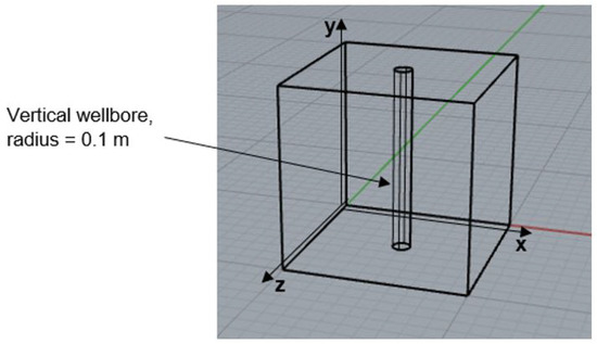
Figure 3.
A CAD model depicting a well model in 3D; length = 10 m, width = 10 m, and wellbore radius = 0.1 m.
The CAD models were then spatially discretised into finite elements (meshed) using an unstructured spatially variable adaptive grid capable of tracking free-form entities such as NURBS. The ICEM CFD software was used for this meshing process. Triangular-shaped elements were used during the mesh generation of the 2D models, whereas a combination of tetrahedral and triangular elements was used for the 3D models.
The mesh quality contributed in no small way to the accuracy and stability of the solution. The orthogonal quality and aspect ratio are conventional methods for assessing mesh quality. The orthogonal quality ranges between 0 and 1, with values closer to 1 denoting a high-quality mesh. The aspect ratio, the ratio between the smallest and largest dimensions of the sides of an element, is required to be no more than 5. The smoothening algorithm in the ICEM CFD software was used to improve the mesh quality [30].
2.2. COMSOL Multiphysics Pseudo-Two-Way Coupling Scheme
COMSOL Multiphysics was used in the simulation of the problem under consideration. The built-in physics interfaces in COMSOL, i.e., the poroelasticity, Darcy flow, transport of diluted species in porous media, and temperature diffusion in porous media, were used. The standard built-in COMSOL governing equations for each of these physics interfaces were found to be analogous to the four governing equations formulated in the current work, i.e., the Navier-type (1), solvent diffusion (2), solute diffusion (3), and thermal diffusion (4) equations, respectively. We note, however, that the governing poroelasticity equation for the COMSOL poroelasticity physics interface does not include the chemical and thermal term, , which is part of the current formulation of the Navier-type Equation (1). These additional chemical and thermal coupling terms were accounted for by adding the chemical and thermal coupling terms as source terms [31] when implementing the poroelascity interface in COMSOL. All four physics interfaces were set to be solved as time-dependent problems simultaneously over 120 h (5 days) with a time step of 6 h.
The solution strategy here, therefore, adopts a scheme that assumes that no coupling exists between the hydraulic, chemical, and thermal gradients imposed on the formation by the drilling fluid. The hydraulic fluid pressure is two-way coupled to the solid mechanics, whereas the chemical activity and temperature are only explicitly coupled to the rock mechanics contributing moisture transport and thermal stresses; hence, the use of the terminology ‘pseudo two-way coupling’.
3. Results and Discussion
We simulated the steady-state conditions for the 2D poroelastic model in CSMP++ and COMSOL Multiphysics. This part of the study focuses mainly on the poroelastic response. Hence, the temperature and chemical activity terms in Equations (10) and (12) are neglected.
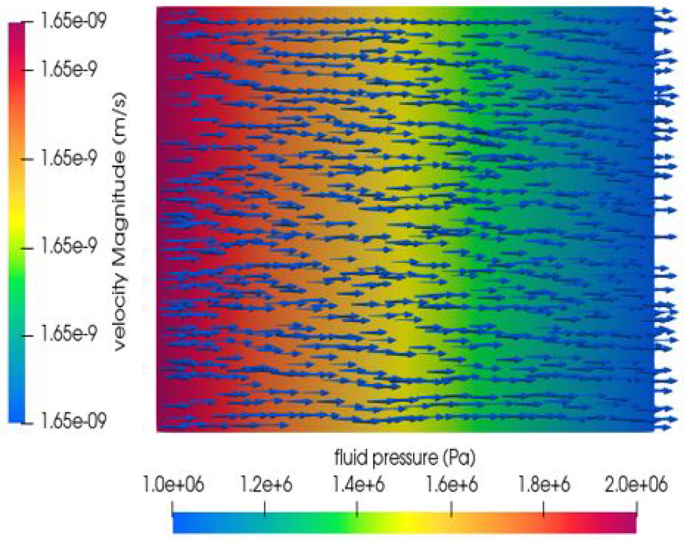
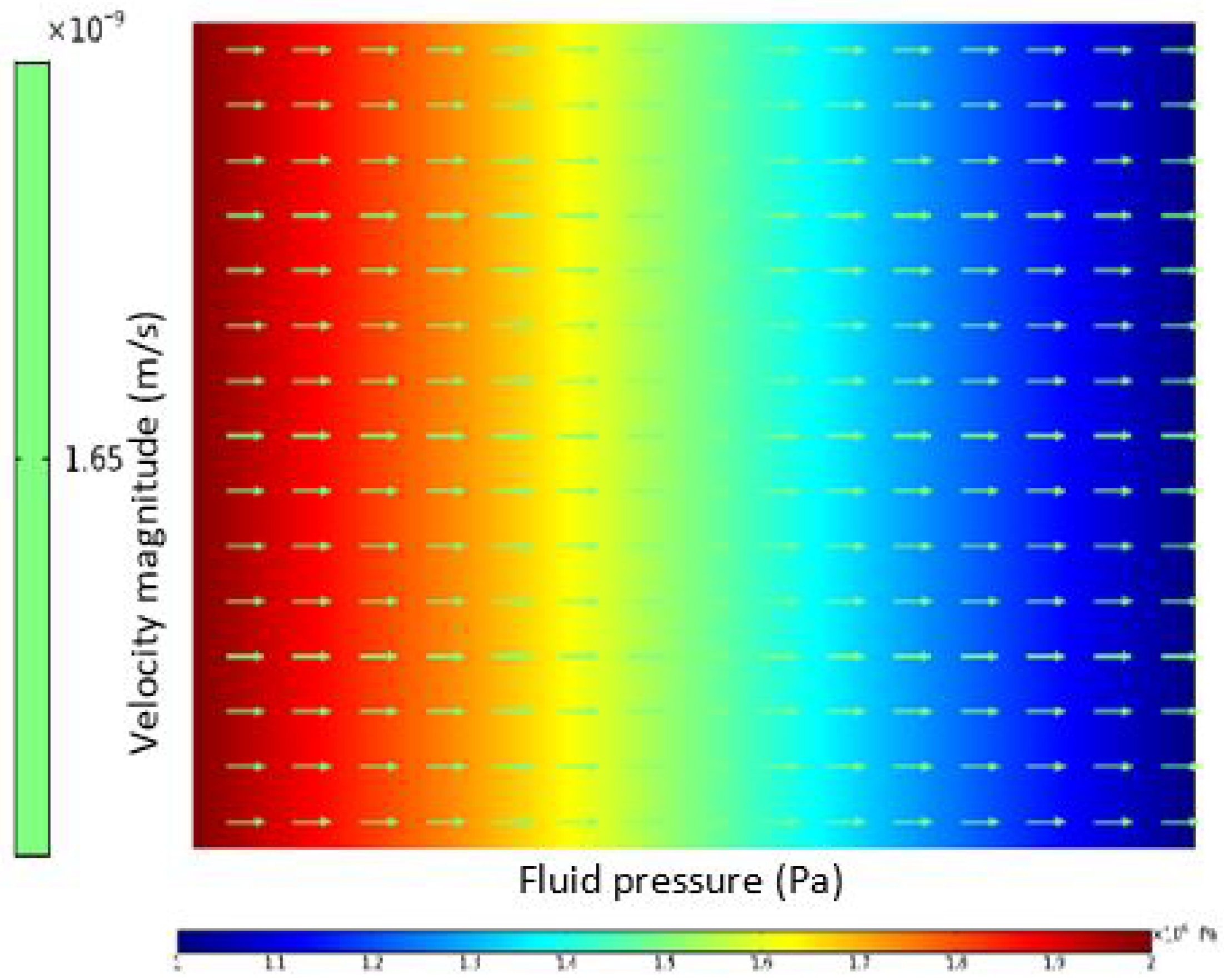
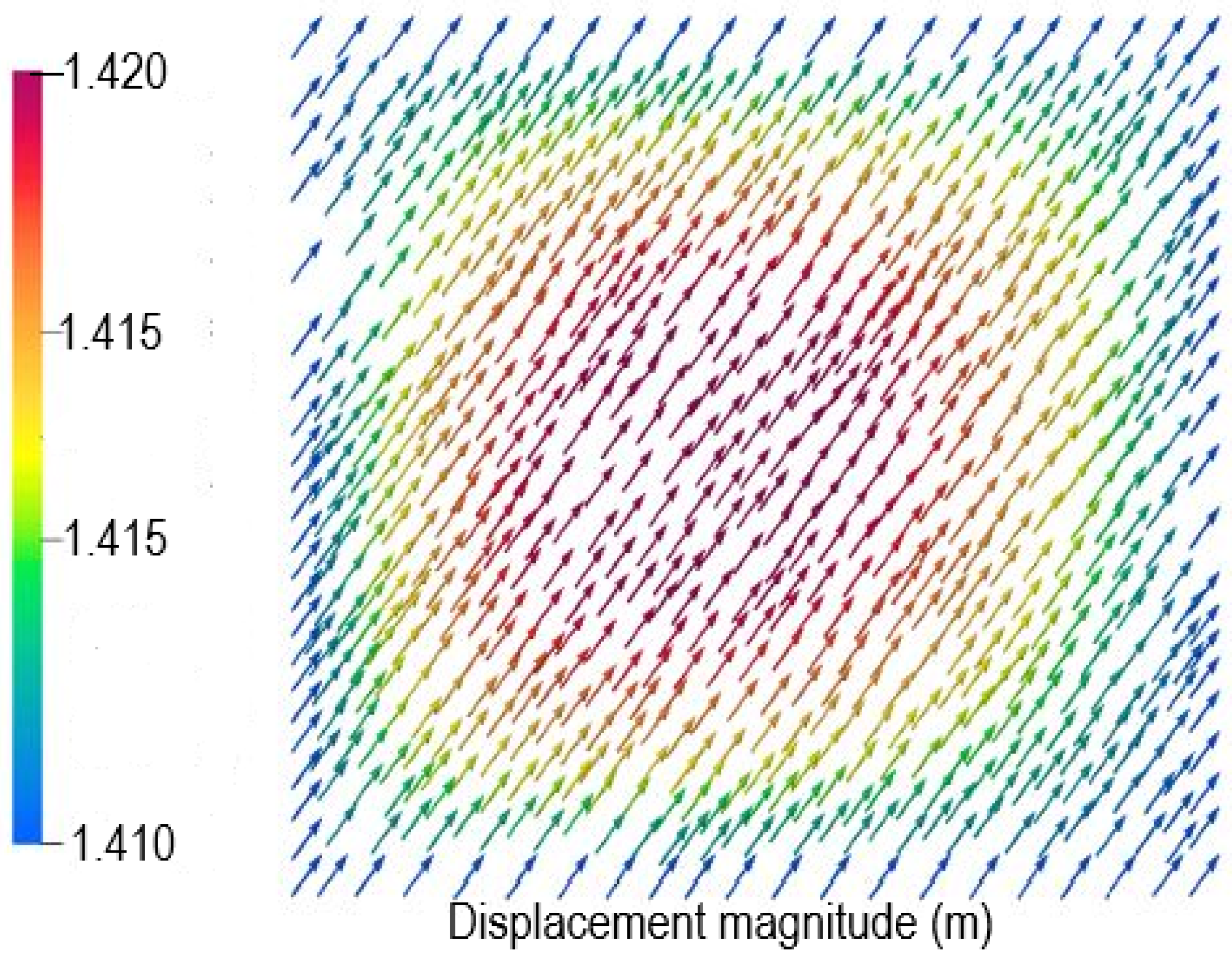
Here, we compare the results obtained using our explicit sequentially coupled approach with those from the partial two-way coupled approach in COMSOL. Simple 2D and 3D geometric models with the dimensions shown in Figure 2 and Figure 3 were used for this test. For the 2D model, Dirichlet flow boundary conditions were implemented on the left and right boundaries at pressures of 2 MPa and 1 MPa, respectively. The results obtained using the CSMP++ explicit sequential approach developed in the current study and COMSOL Multiphysics are shown in Figure 4 and Figure 5 for the fluid pressure gradient and velocity field and Figure 6 and Figure 7 for the displacement field.

Figure 4.
Fluid pressure and velocity field at steady states from the CSMP explicit sequential approach.
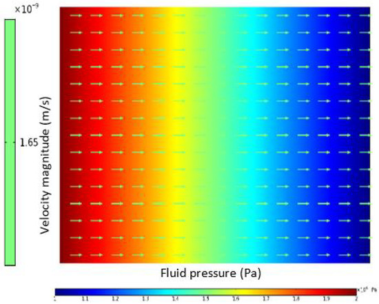
Figure 5.
Fluid pressure and velocity field at steady states from COMSOL Multiphysics.
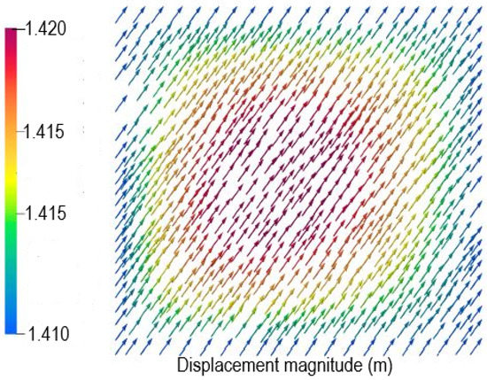
Figure 6.
Computed displacement field from CSMP++.

Figure 7.
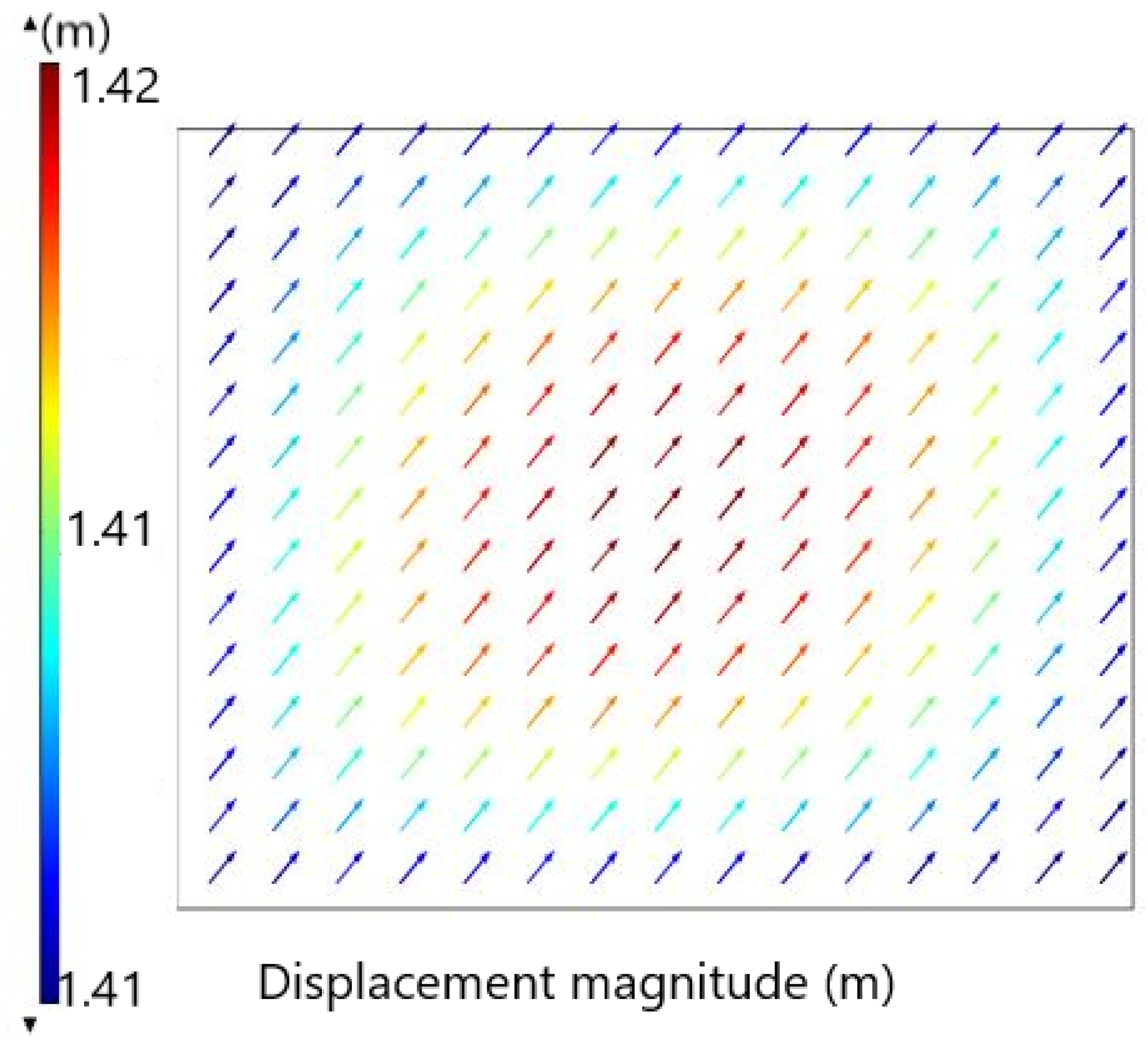
Computed displacement field from COMSOL.
Computed values of fluid pressure and displacement from the two approaches are identical. An average steady-state fluid velocity of m/s and displacement values between 1.41 m and 1.42 m, respectively, are computed from the the explicit sequential approach implemented in CSMP++. The computed displacement error value is . The partial two-way coupled approach in COMSOL Multiphysics also computes velocity value of m/s and displacement values between 1.41 m and 1.42 m.
3.1. Two-Dimensional Poroelastic Analysis of a Borehole
A numerical investigation into the geomechanical properties of a 2D wellbore model under a poroelasticity framework was carried out. The rock mechanical data used in the finite-element numerical solutions for both approaches (i.e., explicit sequential approach implemented in CSMP and partial fully-coupled approach in COMSOL Multiphysics) were adapted from the studies by [24,32] and are shown in Table A3. The boundary conditions applied are shown in Table 1.

Table 1.
Dirichlet boundary conditions used in the FEM numerical simulations.
This process was repeated for the transient simulation over 5 days. Comparisons were then made with the simulations made with COMSOL using the same conditions. The CAD model created for the CSMP++ simulation was first put through a mesh sensitivity analysis in order to ascertain the optimum mesh required. A reference mesh was first generated, then, subsequently, a coarser mesh, i.e., one with a smaller number of elements than the reference, and a finer mesh, i.e., one with more elements than the reference, were made (see Table 2). The temperature distribution was computed over the computational domain. The temperature values were then recorded along a reference slit for each mesh generated. A similar test was conducted for the 3D model used for the computations in Section 3.3. From the results obtained (Table 2), it was apparent that the computational error was reduced with the increasing mesh density. Thus, it was decided to conduct further computations with the 2DF and 3DF models, whereas for the COMSOL computation, a mesh density with an extra-fine setting using triangular elements was selected with the corresponding elements and nodes shown in Table 2 that were similar in number to the 2DF model.
Table 2.
Mesh information for the 2D and 3D CAD models.
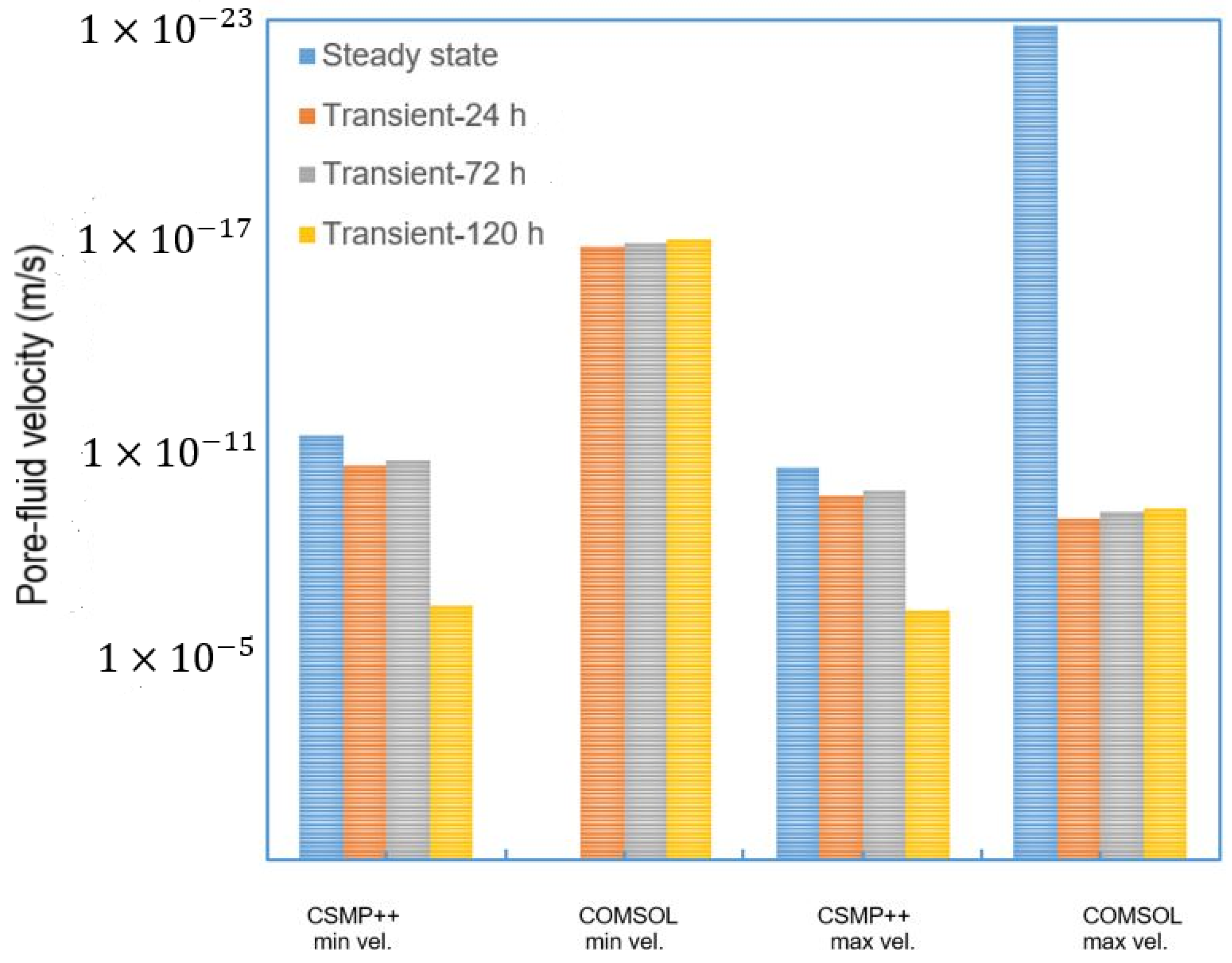
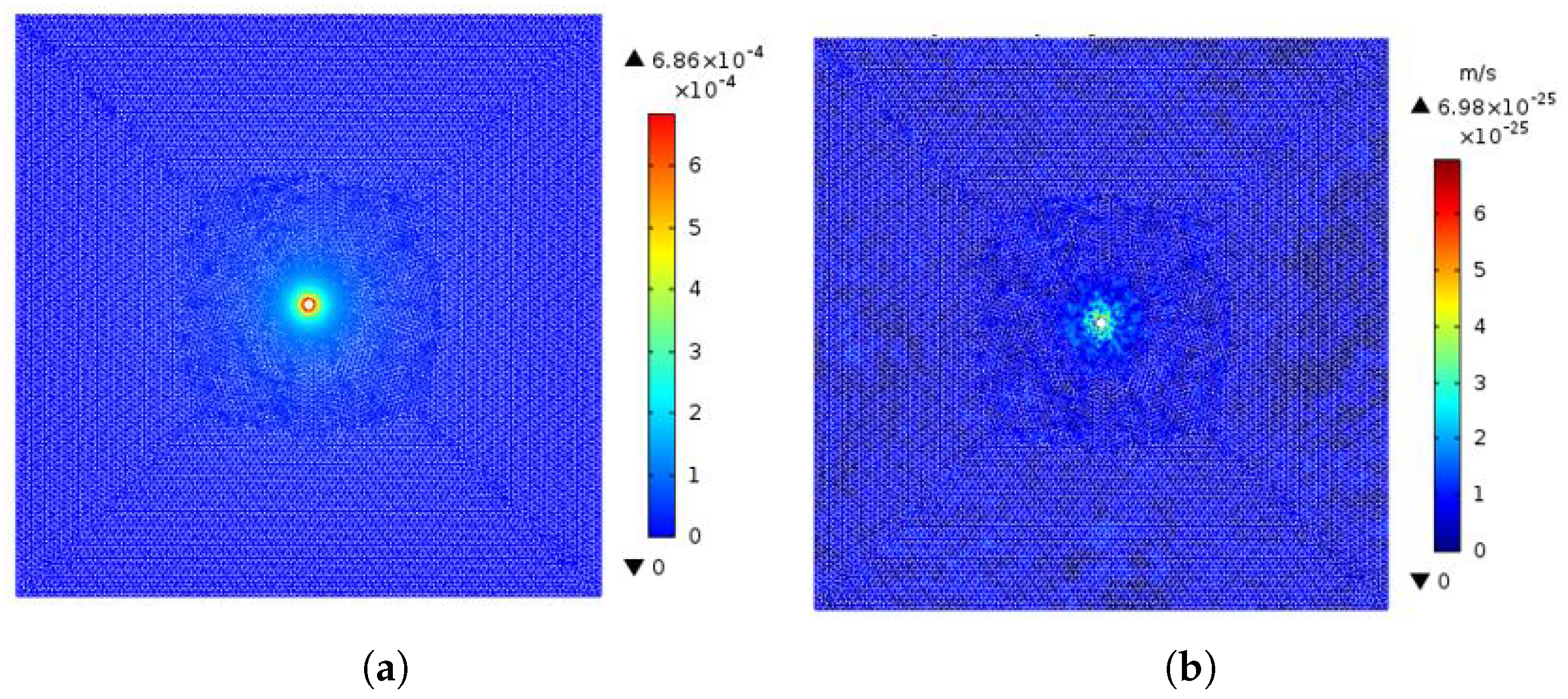
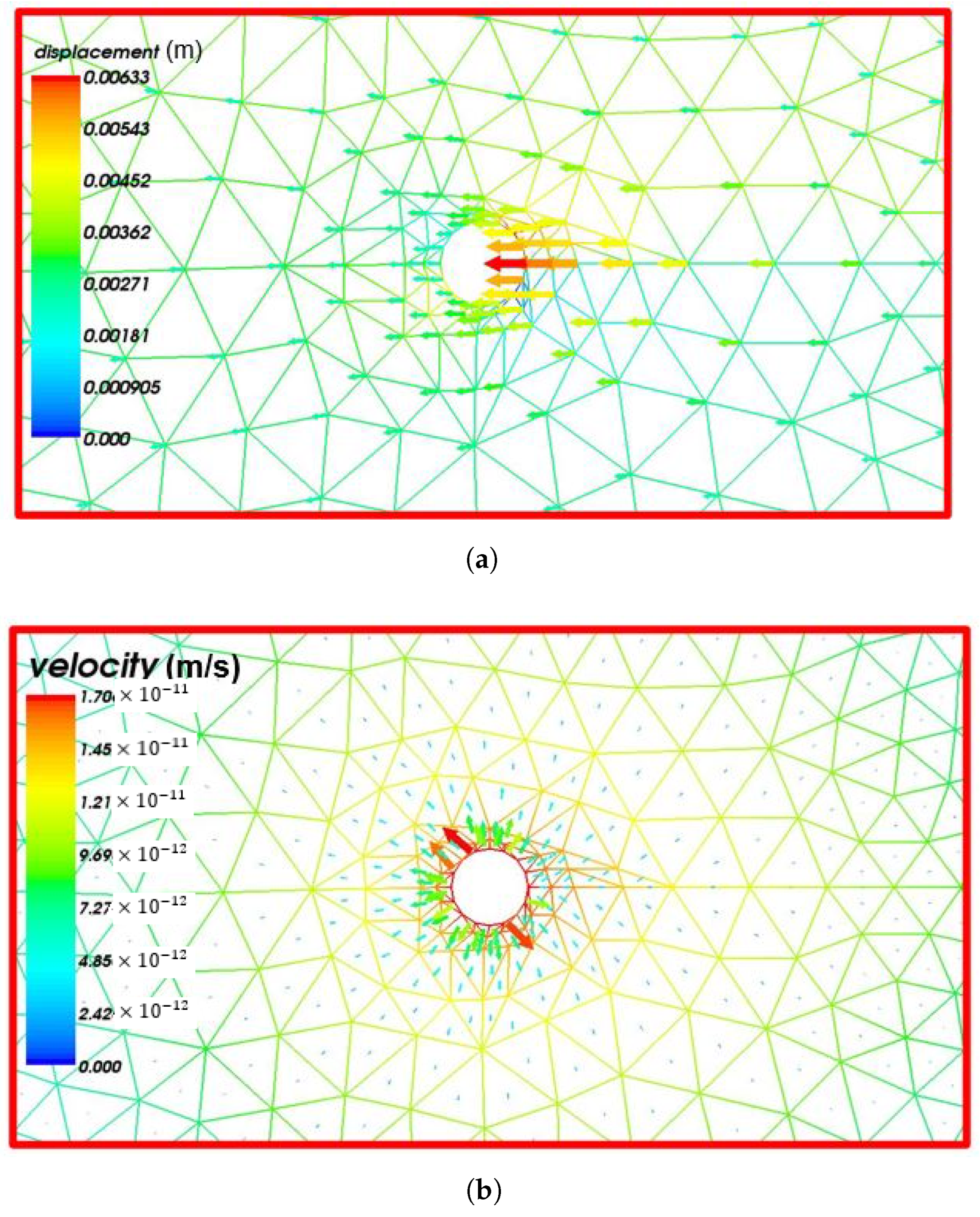
Figure 8 and Figure 9 show the range of pore-fluid velocities, as well as the maximum displacements recorded. Under steady-state conditions, it was observed that the maximum displacement attained was 0.00633 m at the wall, with higher values observed in the minimum horizontal stress direction (Figure 10), whereas the maximum displacement observed in the minimum horizontal direction was 0.0035 m, denoting a difference of 0.00283 m. In addition, it can be seen that the displacement was concentrated around the near-wellbore area. This further strengthens the argument that failure is more likely to occur in this area as a result of the perturbations from the borehole pressure [3,33]. Furthermore, pore-fluid velocities were also found to be higher in the vicinity of the borehole as a result of the pore-pressure elevation resulting from the borehole fluid influx.

Figure 8.
Comparison of pore-fluid velocities computed using CSMP++ and COMSOL under the poroelastic framework.
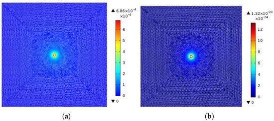
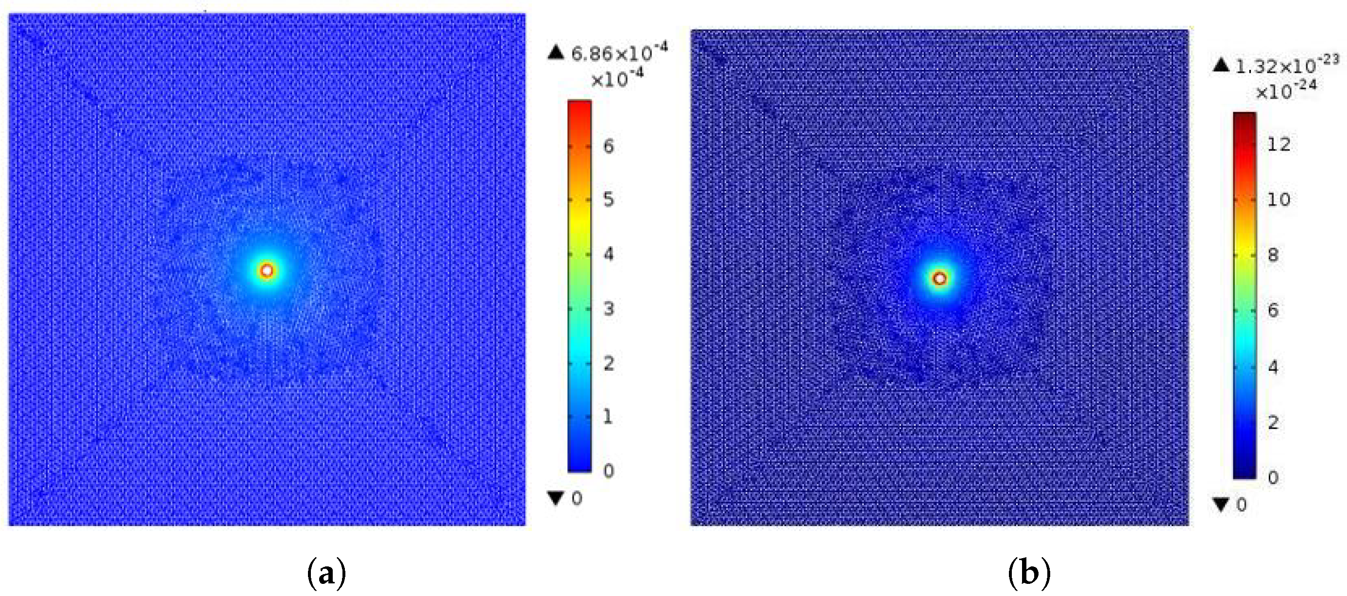
Figure 9.
Two-dimensional steady-state poroelasticity simulation with COMSOL. (a) Total rock displacement (m) and (b) pore-fluid velocity (m/s).
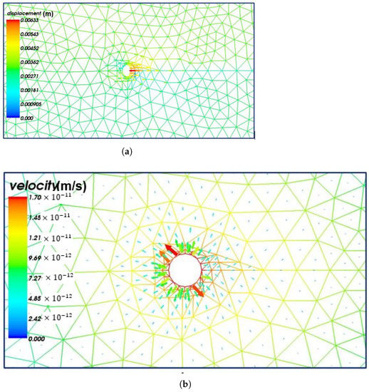
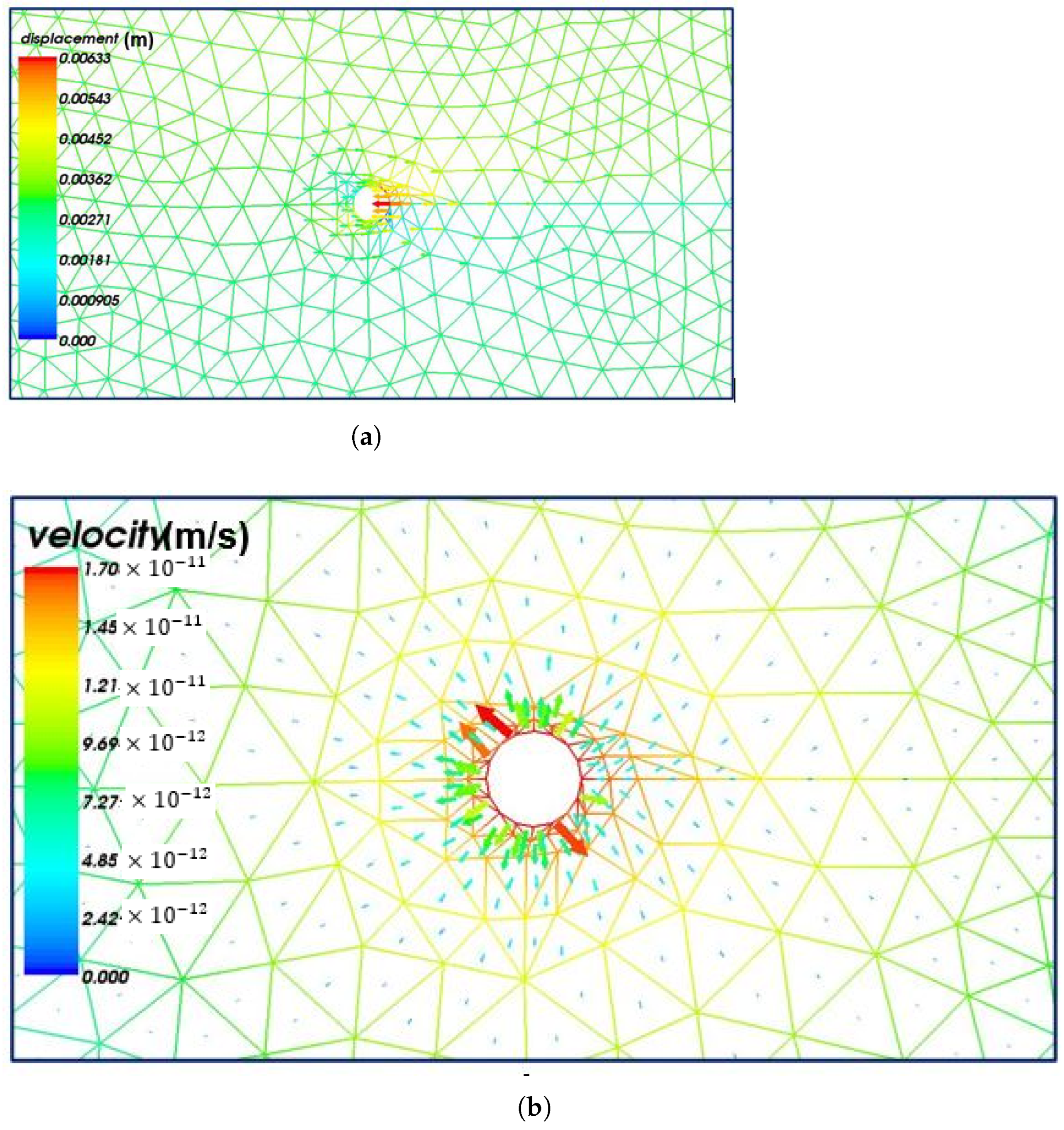
Figure 10.
CSMP++ 2D steady-state poroelasticity. (a) Rock displacement (m) and (b) pore-fluid velocity (m/s) close-up around the 2D borehole.
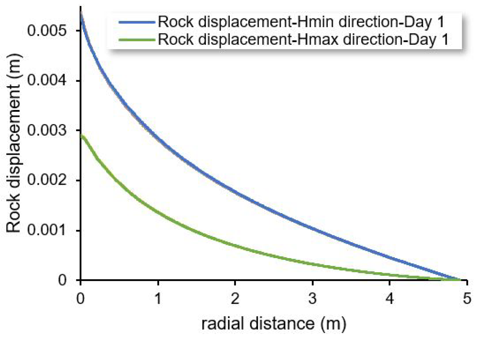
The transient simulation was conducted over a 120 h period and showed a gradual increase in the maximum displacement from 0.0055 m at the borehole wall in the direction to 0 m at a radial distance of 5 m, where the impact of the borehole perturbations was no longer felt. This trend was also noticed in the pore-fluid velocities, which gradually increased by about from ms to ms over 120 h as the borehole pressure influx gradually transmitted into the formation and increased the near-wellbore pore pressure. The gradual increase in the displacements and velocities can be attributed to the time-dependent pore pressure changes, which could potentially result in delayed rock failure [7,24]. Similarly, the maximum displacements were seen to be the highest in the minimum horizontal stress direction due to the effects of the far-field in situ stresses. By implication, these simulation results indicate that rock failure is likely around the near-wellbore area and in the direction of the minimum horizontal in situ stress, which is time dependent.
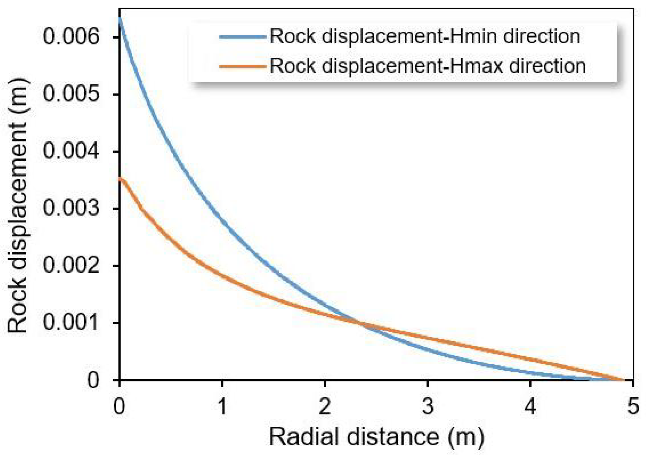
Figure 11 shows the variation in the rock displacement along the radial distance from the wellbore for the 2D poroelasticity steady-state simulation and Figure 12 shows the graphical plot of the rock displacement in the minimum and maximum horizontal in situ stress directions for the 2D poroelasticity transient simulation.
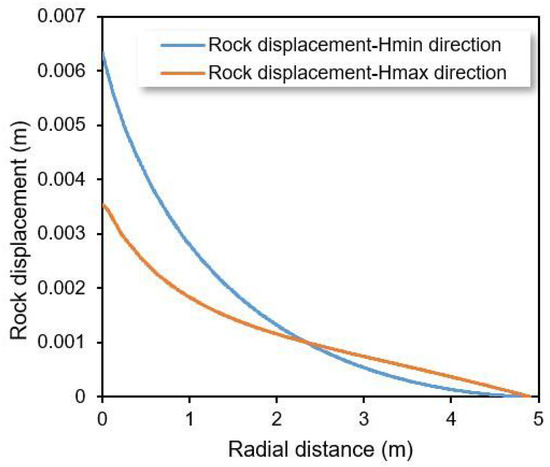
Figure 11.
Variations in the rock displacement from CSMP++ along the radial distance from the wellbore for the 2D poroelasticity steady-state simulation.
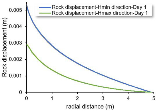
Figure 12.
CSMP++ graphical plot of the rock displacement in the minimum and maximum horizontal in situ stress directions for the 2D poroelasticity transient simulation.
A further comparison was made with the published work of [12]. The pore-pressure dissipation near the wellbore area was computed using the coupled chemo-poroelasticity models. The finite-element method was used in both cases. Figure 13 shows a comparison of the CSMP++ simulation with the published data obtained from [12]. The material properties and conditions used in both cases were similar. The main difference in the computation approach lies in the use of chemical activity (based on the water activity of the drilling and pore fluid) in this work and the chemical concentration in [12] as the driving forces of the chemical potential. For this purpose, transient simulation data for time h from this work and [12] were compared. The results for from [12] were plotted against h from this work and displayed in Figure 13. The results were further analysed by evaluating the root mean square error (RMSE) from both datasets and tabulated as shown in Table 3. corresponds to the steady state in CSMP++ and 30 s in [12], respectively.
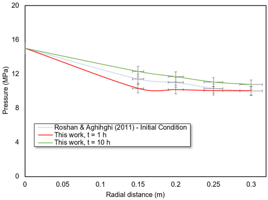
Figure 13.
Comparison of the computed pore-pressure dissipation near the wellbore for CSMP++ and [12] for the 2D chemo-poroelasticity simulation.
Table 3.
Root mean square error (RMSE) obtained from the comparison of this work and the chemo-poroelasticity model.
3.2. Two-Dimensional Chemo-Thermo-Poroelastic Analysis of a Borehole
A study was conducted to investigate the impact of wellbore fluids on the geomechanical properties around a wellbore in 2D under a chemo-thermo-poroelasticity framework using a 2DF mesh (see Table 2). In the first instance, the simulation was conducted under steady-state conditions. The solution, which is similar to the poroelastic solution, also assumes that the pore-space displacement due to the geomechanical perturbation is very small and thus negligible. Therefore, an explicit coupling scheme is adopted between the Navier-type equation and the other three equations in addition to an explicit coupling between the solute transport and the thermal diffusion equation. The solvent transport equation is also explicitly coupled to the solute transport equation. The resulting finite-element algebraic equation is
The algorithm was set up with the and for solving the Navier equation with the chemical coupling coefficient I and thermal coupling coefficient I interrelations applied. The and were applied to solve the solvent, solute, and thermal diffusion equations. In addition, the interrelations utilised were the chemical coupling coefficient II, thermal coupling coefficient II, hydraulic conductivity, membrane efficiency coefficient, thermal osmosis coefficient, and thermal diffusivity.
The temperature, chemical activity, and pressure fields were first computed sequentially. Then, the solution was passed into the Navier equation to obtain the displacement field. Post-processing operations were then executed to obtain the pore-fluid velocity from the pressure field computed and the stresses and strains from the displacement field. This process was then repeated for the case of a transient simulation over a 120 h period. Comparisons were then made with the simulations carried out with COMSOL using the same material properties and boundary conditions. Figure 14 shows the CSMP++ and COMSOL chemo-thermo-poroelasticity simulation comparison using the 2DF and COMSOL 2D models.
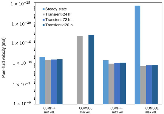
Figure 14.
Comparison of pore-fluid velocities computed using CSMP++ and COMSOL under the chemo-thermo-poroelastic framework using the 2DF and COMSOL 2D models.
The ranges of the maximum pore-fluid velocities and rock displacements obtained are highlighted in Figure 15 and Figure 16, respectively. In the steady-state simulation conducted, the maximum displacement recorded was 0.00633 m in the , with the highest displacement in the direction being at the wall with a maximum magnitude of 0.0035 m (Figure 17). The displacements recorded here are similar to the results obtained during the poroelastic simulation in Section 3.1. Similarly, the displacement was observed to be concentrated in the area closest to where the perturbation occurred due to the hydraulic, chemical, and thermal effects of the wellbore fluid.
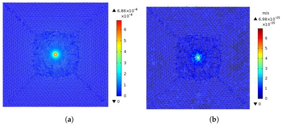
Figure 15.
Two-dimensional steady-state chemo-thermo-poroelasticity simulation with COMSOL. (a) Rock displacement and (b) pore-fluid velocity.
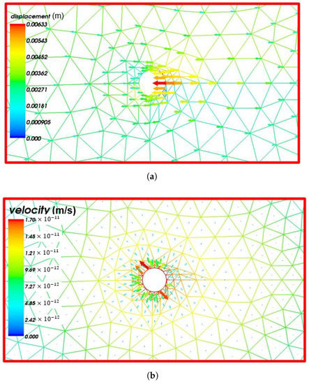
Figure 16.
CSMP++ 2D steady-state chemo-thermo-poroelasticity (a) rock displacement (m) and (b) pore-fluid velocity (m/s) close-up around the 2D borehole.
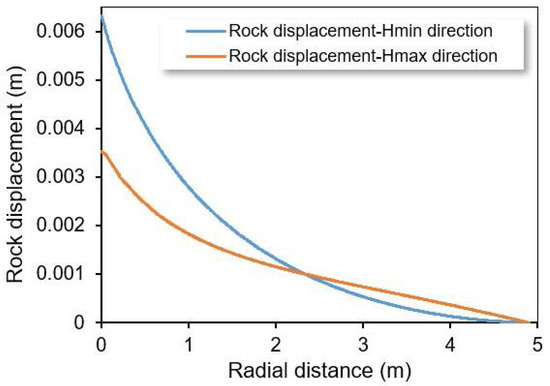
Figure 17.
CSMP++ graphical plots of the rock displacement for a 2D chemo-thermo-poroelasticity steady-state simulation.
In the transient simulation conducted over 120 h on both platforms, the displacement values were observed to increase gradually over time on the CSMP++ platform from 0.00532 to 0.00538 m, with a corresponding decrease in the maximum pore-fluid velocity from to ms. During the steady-state flow, the displacement was higher along the than the when the radial distance was ≤2.5 m and vice versa when the radial distance was >2.5 m. The reason for this observation is attributed to the fact that the displacement was more gradual along the during the steady-state process than the transient process.
The displacement, however, remained the same on the COMSOL platform throughout the simulation at 0.000456 m, but the maximum pore-fluid velocity decreased from to m/s. Similar velocities to the poroelastic model were recorded after 72 h of simulation time. However, after 120 h, there was a clear distinction in the maximum displacement values, which were 0.00538 m in the chemo-thermo-poroelastic model against the 0.00529 m of the poroelastic model. The increased displacement is attributable to the time-dependent effect of the chemical osmosis and heat transport on the rock matrix and the pore fluid.
3.3. Three-Dimensional Chemo-Thermo-Poroelastic Analysis
A simulation was conducted on a 3D vertical wellbore model using the 3DF mesh as seen in Table 2. The first simulation case used the boundary conditions shown in Table 2. Figure 18 shows the pore-velocity profile for the chemo-thermo-poroelasticity steady-state simulation obtained from CSMP++. From the results obtained (see Figure 18 and Figure 19), it can be stated that the maximum rock displacement realisable due to the effects of the borehole fluids on the formation was 0.0264 m, which was about 4 times higher than that obtained in the 2D chemo-thermo-poroelastic simulation. This shows a conservative estimate made by the 2D model, which discounts the impact of the vertical overburden on the stress concentration around the borehole. In the study by [29], it was discovered that 2D simulations underestimated the pore pressure and stress fields in borehole stability studies, which also agrees with the results obtained here. This occurrence is attributable to the extra load causing increased straining of the rock matrix, and thus a heightened displacement field. It was observed here that the pore-fluid velocity field also had a higher magnitude in comparison to the poroelastic model. By increasing the borehole pressure to 20 MPa, it was observed that the rock displacement and velocities concurrently increased by for both cases, as expected. However, increasing the wellbore temperature and the chemical activities barely showed any effect on the rock and the pore fluid. This indicates that the borehole pressure is the most prominent gradient and it should be monitored more carefully.
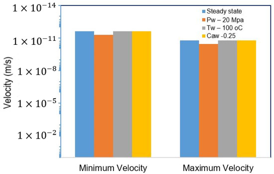
Figure 18.
CSMP++ 3D vertical wellbore chemo-thermo-poroelasticity simulation.
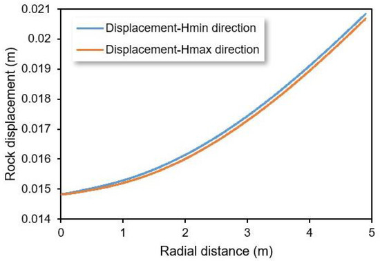
Figure 19.
CSMP++ graphical plot of the rock displacement in the minimum and maximum horizontal in situ stress directions for a 3D chemo-thermo-poroelasticity steady-state simulation.
Figure 19 shows the rock displacement in the minimum and maximum horizontal stress directions, with the displacement appearing higher in the minimum horizontal stress direction. This is an indication that borehole failure is more likely in this direction, which is in agreement with similar studies [34]. Figure 20 shows the pore-fluid velocity computation in CSMP++ for 3D vertical wellbore steady-state chemo-thermo-poroelasticity model. A similar trend was also observed when the borehole pressure was increased to 20 MPa, with a consequent increase in the displacement (see Figure 21). As part of the contribution of this work, the approach developed can be used to design an improved pumping schedule for hydraulic fracturing in tight and unconventional shale formations (e.g., [35,36]). Drilling through and fracturing shale formations using a water-based drilling fluid is challenging due to its tendency to react with the drilling fluid and absorb water. This occurrence leads to shale swelling and pore pressure elevation inside the formation. This subsequently results in wellbore instability due to a redistribution of in situ subsurface stresses around the wellbore. The principal mechanisms responsible for drilling fluid–shale interactions include the capillary pressure, thermal effects, osmotic potential difference, hydraulic pressure difference, swelling, filtrate invasion, pressure penetration, and physico-chemical interactions between the fluid and shale. The model developed can, therefore, be used to improve the pumping schedule for hydraulic fracturing and unconventional drilling.
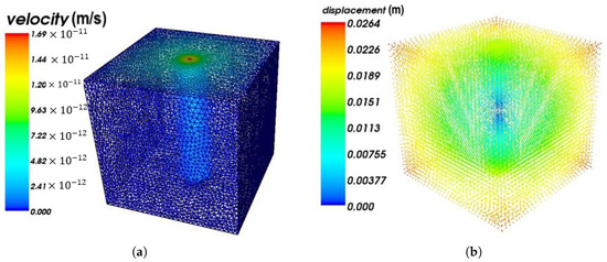
Figure 20.
CSMP++ 3D vertical wellbore steady-state chemo-thermo-poroelasticity. (a) Pore-fluid velocity (m/s) and (b) rock displacement (m).

Figure 21.
CSMP++ graphical plot of the rock displacement in the minimum and maximum horizontal in situ stress directions for a 3D chemo-thermo-poroelasticity steady-state simulation for Pw-20 MPa.
4. Conclusions
A coupled chemo-thermo-poroelastic wellbore stability model encompassing multiple components was presented and implemented using the finite-element method. A C++ finite-element code was implemented in CSMP++ and applied to solve the model using a sequential approach. A comparative study between the solution approach developed in this work and the partial two-way coupling approach adopted in COMSOL Multiphysics, a commercial software package, was carried out. Numerical simulations were then conducted on 2D and 3D models of different wellbore configurations to analyse how the geomechanical properties of the rocks change under different borehole conditions. The following conclusions can be drawn:
- Rock displacement occurs in the areas nearest to the borehole where perturbations due to hydraulic, chemical, and thermal gradients are prominent. This is also the same with respect to the pore-fluid velocities.
- The in situ formation stresses influence the path on which the rock displacement occurs, with the displacement seen to be more prominent in the minimum horizontal stress direction.
- For the 2D test cases, the maximum difference between the computed temperature using the explicit sequential approach in CSMP++ and the partial two-way coupling approach in COMSOL Multiphysics is . The computed average steady-state fluid velocity is m/s for both simulators. The corresponding range for the displacement values is between 1.41 m and 1.42 m and is similar for both simulators.
- When comparing the solution of the simulation obtained from the 2D model to that obtained from the 3D model, it is observed that the 2D model underestimates the magnitude of the displacements and pore-fluid velocities.
Author Contributions
Conceptualisation, L.T.A., A.I. and H.H.; methodology, H.H., L.T.A. and A.I.; software, L.T.A. and S.M.; writing—original draft preparation, A.I. and L.T.A.; writing—review and editing, L.T.A., A.A. and S.M.; supervision, H.H., L.T.A., S.M. and A.A. All authors have read and agreed to the published version of the manuscript.
Funding
This research received no external funding.
Data Availability Statement
Not applicable.
Acknowledgments
The authors would like to acknowledge the Petroleum Technology Development Fund for sponsoring Adamu Ibrahim’s PhD research work.
Conflicts of Interest
The authors declare no conflict of interest.
Abbreviations and List of Symbols
List of Symbols
| pressure differential | |
| wellbore pressure | |
| pore pressure | |
| h | vertical thickness of rock formation |
| g | gravitational constant |
| formation pore pressure | |
| Biot’s coefficient | |
| Biot effective fluid coefficient | |
| v | Poisson’s ratio in the plane of isotropy (horizontal direction) |
| Poisson’s ratio in the plane normal to isotropy (vertical direction) | |
| Young’s modulus in the plane of isotropy (horizontal direction) | |
| Young’s modulus in the plane normal to isotropy (vertical direction) | |
| tectonic strain in the maximum strain direction | |
| tectonic strain in the minimum strain direction | |
| angle of inclination of the planes | |
| K | bulk modulus |
| G | shear modulus |
| u | displacement |
| Skempton’s coefficient | |
| thermal coupling coefficient | |
| thermal coupling coefficient | |
| thermal coupling coefficient | |
| density | |
| density | |
| dynamic fluid viscosity | |
| fluid viscosity | |
| D | diffusion coefficient |
| solute concentration | |
| n | number of constituent ions of the dissociated solute |
| coupling coefficients | |
| coupling coefficients | |
| hydraulic diffusivity | |
| membrane efficiency coefficient | |
| c | fluid compressibility |
| molar fraction of water | |
| water activity | |
| wellbore radius | |
| chemical activity | |
| X | chemical coupling coefficients |
| chemical coupling coefficients | |
| L | chemical coupling coefficients |
| bulk volume | |
| pore volume | |
| grain volume | |
| total stress tensor | |
| total strain tensor | |
| solute mass fraction | |
| solvent mass fraction | |
| fluid mass density | |
| molar mass of solute | |
| swelling coefficient of the rock | |
| R | universal gas constant |
| diluent mass fraction | |
| absolute temperature | |
| solute mass fraction | |
| thermal expansion coefficient of the solid | |
| specific entropy | |
| porosity | |
| solid bulk modulus | |
| fluid bulk modulus | |
| k | permeability (mD) |
| ℜ | membrane efficiency |
| thermal diffusion coefficient | |
| solute diffusion coefficient |
Abbreviations
The following abbreviations are used in this manuscript:
| CAD | computer-aided design |
| FEM | finite-element method |
| CSMP++ | complex system modelling platform |
| PDE | partial differential equation |
| SAMG | algebraic multigrid processes for systems |
| NURBS | non-uniform rational B-splines |
| ICEM | integrated computer engineering and manufacturing |
| CFD | computational fluid dynamics |
| maximum horizontal in situ stress | |
| minimum horizontal in situ stress |
Appendix A
Appendix A.1. Finite-Element Integral Matrices and Corresponding PDE Operators
Table A1.
Finite-Element Integral Matrices and Corresponding PDE Operators Applied in this Study.
Table A1.
Finite-Element Integral Matrices and Corresponding PDE Operators Applied in this Study.
| Finite-Element Weak Forms | PDE Operators |
|---|---|
| − | |
Appendix A.2. List of Coefficient Variables Coded Using the Interrelation Subclass
Table A2.
List of Coefficient Variables Constructed in CSMP++ Using the Interrelation.
Table A2.
List of Coefficient Variables Constructed in CSMP++ Using the Interrelation.
| Interrelations | Equations |
|---|---|
| Biot fluid coefficient fluid | |
| Chemical coupling coefficient one | |
| Thermal coupling coefficient one | |
| Skempton’s coefficient | |
| Chemical coupling coefficient two | |
| Thermal coupling coefficient two | |
| Hydraulic conductivity | |
| Membrane efficiency coefficient | |
| Diff-poro coefficient | |
| Thermal osmotic coefficient |
Appendix A.3. Typical Properties of Shale Rock Used in the Numerical Simulation
Table A3.
Typical Properties of Shale Rock Used in the Numerical Simulation.
Table A3.
Typical Properties of Shale Rock Used in the Numerical Simulation.
| Young’s modulus, E | 1853 MPa |
| Drained Poisson’s ratio, v | |
| Undrained Poisson’s ratio, | |
| Skempton’s coefficient, | |
| Permeability, k | darcy |
| kg/m | |
| Pa.s | |
| kg/mol | |
| MPa | |
| m/s | |
| Pressure diffusion coefficient, L | 0 |
| K | |
| K | |
| K | |
| m/(s.K) | |
| 3686 J/(kgK) | |
Where is the Biot fluid coefficient, is the Biot’s coefficient, is the molar mass of the solute, is the swelling coefficient of the rock, is the fluid mass density, R is the universal gas constant, is the absolute temperature, is the diluent mass fraction, is the chemical coupling coefficient one, is the solute mass fraction, is the thermal coupling coefficient, K is the bulk modulus, is the thermal expansion coefficient of the solid, is the specific entropy, is the Skempton’s coefficient, is the porosity, is the solid bulk modulus, is the fluid bulk modulus, is the chemical coupling coefficient two, is the permeability, is the fluid viscosity, is the thermal diffusion coefficient, is the solute diffusion coefficient, and Re is the membrane efficiency.
Appendix A.4. Sample Code Used in Computing Chemical Coupling Coefficient 1 (ChemoOne) Interrelation (Version 2005—A New Open CSMP Release Will Soon Be Available)
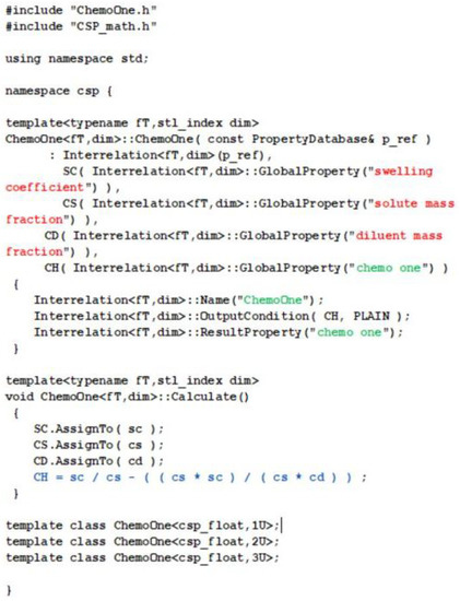
Figure A1.
A Sample Interrelation Code Used in Computing Chemical Coupling Coefficient 1 (ChemoOne).
Figure A1.
A Sample Interrelation Code Used in Computing Chemical Coupling Coefficient 1 (ChemoOne).
References
- Dean, R.H.; Gai, X.; Stone, C.M.; Minkoff, S.E. A comparison of techniques for coupling porous flow and geomechanics. SPE J. 2006, 11, 132–140. [Google Scholar] [CrossRef]
- Biot, M.A. General theory of Three-Dimensional consolidation. J. Appl. Phys. 1941, 12, 155–164. [Google Scholar] [CrossRef]
- Detournay, E.; Cheng, A.H. Poroelastic response of a borehole in a non-hydrostatic stress field. Int. J. Rock Mech. Min. Sci. Geomech. Abstr. 1988, 25, 171–182. [Google Scholar] [CrossRef]
- Cui, L.; Kaliakin, V.N.; Abousleiman, Y.; Cheng, A.H. Finite-element formulation and application of po-roelastic generalized plane strain problems. Int. J. Rock Mech. Min. Sci. 1997, 34, 953–962. [Google Scholar] [CrossRef]
- Chen, G.; Chenevert, M.E.; Sharma, M.M.; Yu, M. Poroelastic chemical, and thermal effects on wellbore stability in shales. In Proceedings of the 38th U.S. Symposium on Rock Mechanics (USRMS), Washington, DC, USA, 7–10 July 2001. [Google Scholar]
- Zhou, X.; Ghassemi, A. Finite-element analysis of coupled chemo-poro-thermo-mechanical effects around a wellbore in swelling shale. Int. J. Rock Mech. Min. Sci. 2009, 46, 769–778. [Google Scholar] [CrossRef]
- Cao, W.; Deng, J.; Yu, B.; Tan, Q.; Liu, W.; Jin, C.; Ren, G.; Guo, X.; Liu, H. Wellbore stability analysis based on the fully coupled non-linear chemo-thermo-poroelastic theory in shale formation. In Proceedings of the 51st U.S. Rock Mechanics/Geomechanics Symposium, San Francisco, CA, USA, 25–28 June 2017. [Google Scholar]
- Cheng, W.; Jiang, G.; Li, X.; Zhou, Z.; Wei, Z. A porochemothermoelastic coupling model for continental shale wellbore stability and a case analysis. J. Pet. Sci. Eng. 2019, 182, 106265. [Google Scholar] [CrossRef]
- Tran, D.; Nghiem, L.; Buchanan, L. Aspects of coupling between petroleum reservoir flow and geome-chanics. In Proceedings of the 43rd U.S. Rock Mechanics Symposium and 4th U.S.-Canada Rock Mechanics Symposium, Asheville, NC, USA, 28 June–1 July 2009. [Google Scholar]
- Gala, D.P.; Manchanda, R.; Mukul, M.S. Modeling of Fluid Injection in Depleted Parent Wells to Minimize Damage Due to Frac-Hits. In Proceedings of the SPE/AAPG/SEG Unconventional Resources Technology Conference, Houston, TX, USA,, 23–25 July 2018. [Google Scholar] [CrossRef]
- Roshan, H.; Rahman, S.S. A fully coupled chemo-poroelastic analysis of pore pressure and stress distribu-tion around a wellbore in water active rocks. Rock Mech. Rock Eng. 2011, 44, 199–210. [Google Scholar] [CrossRef]
- Roshan, H.; Aghighi, M.A. Chemo-poroelastic analysis of pore pressure and stress distribution around a wellbore in swelling shale: Effect of undrained response and horizontal permeability anisotropy. Geome-Chanics Geoeng. 2012, 7, 209–218. [Google Scholar] [CrossRef]
- Agheshlui, H.; Matthai, S. Uncertainties in the estimation of in situ stresses: Effects of heterogeneity and thermal perturbation. Geomech. Geophys. Geo-Energy Geo-Resour. 2017, 3, 415–438. [Google Scholar] [CrossRef]
- Grandi, S.; Rao, R.V.N.; Toksoz, M.N. Geomechanical Modeling of In Situ Stresses around a Borehole. 2002. Available online: http://hdl.handle.net/1721.1/67848 (accessed on 25 May 2022).
- Hoeink, T.; van der Zee, W.; Moos, D. Finite element analysis of stresses induced by gravity in layered rock masses with different elastic moduli. In Proceedings of the 46th US Rock Mechanics/Geomechanics Symposium, Chicago, IL, USA, 24–27 June 2012. [Google Scholar]
- Jha, B.; Juanes, R. A locally conservative finite element framework for the simulation of coupled flow and reservoir geomechanics. Acta Geotech. 2007, 2, 139–153. [Google Scholar] [CrossRef]
- Lautenschlager, C.E.R.; Righetto, G.L.; Inoue, N.; da Fontoura, S.A. Advances on partial coupling in res-ervoir simulation: A new scheme of hydromechanical coupling. In Proceedings of the North Africa Technical Conference and Exhibition, Cairo, Egypt, 15–17 April 2013. [Google Scholar]
- Jinze, X.; Keliu, W.; Zhandong, L.; Yi, P.; Ran, L.; Jing, L.; Zhangxin, C. A Model for Gas Transport in Dual-Porosity Shale Rocks with Fractal Structures. Ind. Eng. Chem. Res. 2018, 57, 6530–6537. [Google Scholar] [CrossRef]
- Adeleye, J.O.; Akanji, L.T. A quantitative analysis of flow properties and heterogeneity in shale rocks using computed tomography imaging and finite-element based simulation. J. Nat. Gas Sci. Eng. 2022, 106, 104742. [Google Scholar] [CrossRef]
- Narasingam, A.; Siddhamshetty, P.; Sang-Il Kwon, J. Temporal clustering for order reduction of nonlinear parabolic PDE systems with time-dependent spatial domains: Application to a hydraulic fracturing process. Am. Inst. Chem. Eng. (AIChE) J. 2017, 63, 3818–3831. [Google Scholar] [CrossRef]
- Sidhu, H.S.; Narasingam, A.; Kwon, J.S. Model order reduction of nonlinear parabolic PDE systems with moving boundaries using sparse proper orthogonal decomposition methodology. In Proceedings of the Annual American Control Conference (ACC), Milwaukee, WI, USA, 27–29 June 2018; pp. 6421–6426. [Google Scholar] [CrossRef]
- Ibrahim, A.; Akanji, L.; Hamidi, H.; Akisanya, A. Chemo-thermo-poromechanical wellbore stability mod-elling using multi-component drilling fluids. In Proceedings of the SPE Kuwait Oil & Gas Show and Conference, Mishref, Kuwait, 15–18 October 2017. [Google Scholar]
- Smith, I.M.; Griffiths, D.V.; Margetts, L. Programming the Finite-Element Method; Wiley: Somerset, UK, 2013. [Google Scholar]
- Zhou, X.X.; Ghassemi, A. Chemo-poromechanical finite-element modeling of a wellbore in swelling shale. In Proceedings of the 42nd US Rock Mechanics Symposium (USRMS), San Francisco, CA, USA, 29 June–2 July 2008. [Google Scholar]
- Matthäi, S.K.; Geiger, S.; Roberts, S.G.; Paluszny, A.; Belayneh, M.; Burri, A.; Mezentsev, A.; Lu, H.; Coumou, D.; Driesner, T.; et al. Numerical simulation of multi-phase fluid flow in structurally complex reservoirs. Geol. Soc. Lond. Spec. Publ. 2007, 292, 405–429. [Google Scholar] [CrossRef]
- Coumou, D.; Matthäi, S.; Geiger, S.; Driesner, T. A parallel FE–FV scheme to solve fluid flow in complex ge-ologic media. Comput. Geosci. 2008, 34, 1697–1707. [Google Scholar] [CrossRef]
- Kim, J.; Tchelepi, H.A.; Juanes, R. Stability, accuracy, and efficiency of sequential methods for coupled flow and geomechanics. SPE J. 2011, 16, 249–262. [Google Scholar] [CrossRef]
- Matthai, S.K.; Geiger, S.; Roberts, S. Complex Systems Platform: CSP5 Users Guide; 2005; unpublished. [Google Scholar]
- Fowler, S.J.; Kosakowski, G.; Driesner, T.; Kulik, D.A.; Wagner, T.; Wilhelm, S.; Masset, O. Numerical simula-tion of reactive fluid flow on unstructured meshes. Transp. Porous Media 2016, 112, 283–312. [Google Scholar] [CrossRef]
- Chidamoio, J.; Akanji, L.; Rafati, R. Prediction of optimum length to diameter ratio for two-phase fluid flow development in vertical pipes. Adv. Pet. Explor. Dev. 2017, 14, 1–17. [Google Scholar]
- Sijacic, D.; Fokker, P. Simulation of Flow, Thermal and Mechanical Effects in COMSOL for Enhanced Geothermal Systems 2013. Available online: https://www.comsol.jp/paper/download/181555/sijacic_presentation.pdf (accessed on 9 April 2022).
- Huang, L.; Yu, M.; Miska, S.Z.; Takach, N.; Bloys, J.B. Modeling chemically induced pore pressure alter-ations in near wellbore region of shale formations. In Proceedings of the SPE Eastern Regional Meeting, Columbus, OH, USA, 17–19 August 2011. [Google Scholar]
- Detournay, E.; Cheng, A.H. Fundamentals of poroelasticity. Int. J. Rock Mech. Min. Sci. Geomech. Abstr. 1994, 31, 138–139. [Google Scholar] [CrossRef]
- Roshan, H.; Rahman, S.S. 3D borehole model for evaluation of wellbore instabilities in underbalanced drilling. In Proceedings of the SPE EUROPEC/EAGE Annual Conference and Exhibition, Vienna, Austria, 23–26 May 2011. [Google Scholar]
- Mao, S.; Siddhamshetty, P.; Zhang, Z.; Yu, W.; Chun, T.; Kwon, J.S.; Kan, W. Impact of Proppant Pumping Schedule on Well Production for Slickwater Fracturing. SPE J. 2021, 26, 342–358. [Google Scholar] [CrossRef]
- Siddhamshetty, P.; Mao, S.; Wu, K.; Kwon, J.S.-I. Multi-Size Proppant Pumping Schedule of Hydraulic Fracturing: Application to a MP-PIC Model of Unconventional Reservoir for Enhanced Gas Production. Processes 2020, 8, 570. [Google Scholar] [CrossRef]


Disclaimer/Publisher’s Note: The statements, opinions and data contained in all publications are solely those of the individual author(s) and contributor(s) and not of MDPI and/or the editor(s). MDPI and/or the editor(s) disclaim responsibility for any injury to people or property resulting from any ideas, methods, instructions or products referred to in the content. |
© 2023 by the authors. Licensee MDPI, Basel, Switzerland. This article is an open access article distributed under the terms and conditions of the Creative Commons Attribution (CC BY) license (https://creativecommons.org/licenses/by/4.0/).