Abstract
In this work, we provide a smart home occupancy prediction technique based on environmental variables such as CO, noise, and relative temperature via our machine learning method and forecasting strategy. The proposed algorithms enhance the energy management system through the optimal use of the electric heating system. The Long Short-Term Memory (LSTM) neural network is a special deep learning strategy for processing time series prediction that has shown promising prediction results in recent years. To improve the performance of the LSTM algorithm, particularly for autocorrelation prediction, we will focus on optimizing weight updates using various approaches such as Genetic Algorithm (GA) and Particle Swarm Optimization (PSO). The performances of the proposed methods are evaluated using real available datasets. Test results reveal that the GA and the PSO can forecast the parameters with higher prediction fidelity compared to the LSTM networks. Indeed, all experimental predictions reached a range in their correlation coefficients between 99.16% and 99.97%, which proves the efficiency of the proposed approaches.
1. Introduction
One of the most efficient systems to save energy is to reduce a building’s heating and cooling load, which is mostly caused by heat transfer over its envelope. Smart buildings are required to provide permanent, healthy and comfortable indoor environments, independent of exterior weather conditions [1,2]. Indeed, the major part of energy in such buildings is used by Heating, Ventilation, and Air Conditioning (HVAC) systems, which have a significant influence on both home comfort and the environment. Therefore, managing these systems in residential structures should be tackled in order to increase energy efficiency through improved energy planning [3]. One of the most essential features of smart buildings is their ability to self-control the systems used to maintain the comfort of the inside atmosphere while also minimizing energy use. Because HVAC systems are the primary source of energy consumption in buildings, intelligent HVAC system control is a current trend in research studies that necessitates the insertion of occupancy information into the control process [4]. Moreover, the rise of smart buildings, as well as the pressing need to reduce energy use, has rekindled interest in building energy demand prediction. Intelligent controls are a solution for optimizing power consumption in buildings without reducing interior comfort [5]. For example, in [6], a Model Predictive Control (MPC) is developed to obtain a hybrid HVAC control with energy savings while maintaining of thermal comfort. Building energy consumption prediction strives to achieve various goals such as evaluating the impact of energy-saving interventions and assume energy demands based on regular requirements. It can anticipate the fluctuations in power consumption of certain events at specfic times that may modify the systems’ customary energy usage [7]. Furthermore, based on detailed and extensive studies, it was concluded that occupant behavior is one of the most significant elements affecting residential structure energy use. Occupancy behavior includes activities such as turning on and off lights, switching on and off heating and cooling systems, and regulating the temperature.
Previous research has shown that various occupant demands and behaviors necessitate specific technological solutions, which may induce or change behavior patterns, and that occupant behavior affects the flexibility and deployment of technologies. However, the lack of comprehensive knowledge of occupant behaviors in residential building leads to misunderstanding and inaccurate decisions in both technical design and policy making [8]. The context of our research is energy efficiency. In recent years, energy efficiency has been realized by improving the thermal performances of the building envelope’s insulation layer. The research strategies aim to permanently adjust the comfort conditions to the living situation, as well as to ensure greater energy supervision and management within the smart buildings. To achieve this, it is important to automatically characterize the activities of the building’s residents. The significant challenge in today’s new technical design for smart buildings is understanding customer behaviors [9]. In the future, our occupancy prediction approach will guarantee energy savings in a smart building environment. Ambient intelligence is an important prerequisite for improving human quality of life.
The rest of this work is structured as follows: Section 2 explains the technique employed in this project. Firstly, it offers the overall framework of the LSTM forecasting model. Next, it presents, step-by-step, the implementation procedure of the suggested technique; it includes descriptions of database processing, the parameters, and the assessment indicators. Section 3 features experimental details, as well as an analysis of the results. Finally, Section 4 provides some conclusions and future works.
2. Related Works
Building energy consumption is influenced by the thermal insulation, heating, ventilation, air conditioning, lighting, and occupants’ behaviors [10]. Characterising human activity has become an increasingly prominent application of machine learning in a many disciplinary fields. Indeed, for the past two decades, researchers from several application fields have investigated activity recognition by developing a variety of methodologies and techniques for each of these key tasks. The prediction of human behaviour represents a key challenge, and many approaches have already been proposed in the industrial, medical, home care, and energy efficiency domains, and many others [11]. For example, in [12], an end-to-end technique for forecasting multi-zone interior temperatures using LSTM-based sequence to sequence has been introduced. The goal of this prediction is to improve the building’s energy efficiency while maintaining occupant comfort. Authors in [13] also proposed implementing simple XGBoost machine learning methods to predict the interior room temperature, relative humidity, and CO concentration in a commercial structure. The proposed technique presents a practical option because it does not require a large data set for training. Additionally, these models eliminate the necessity for multiple sensors, which create sophisticated and expensive networks. In [14], a short-term load consumption forecasting approach for nonresidential buildings using artificial occupancy attributes and based on Support Vector Machines (SVM) has been developed. However, the determination of human behaviour in this work is imprecise. The authors in [15], present a load forecasting model for office buildings based on artificial intelligence and regression analysis to effectively extract the cooling and heating load characteristics. However, the model assumes that the building’s internal disturbing influences are steady. In [16], an optimal deep learning LSTM model for forecasting electricity consumption utilizing feature selection and a Genetic Algorithm (GA) is implemented. The goal of this suggested technique is to determine the optimal time delays and number of layers for LSTM architecture’s predictive performance optimisation, as well as to minimize overfitting, resulting in more accurate and consistent forecasting. Furthermore, recently, machine learning approaches based on Artificial Neural Networks (ANNs) have been widely used to forecast the thermal behavior of modern buildings for modeling HVAC systems. As an example, in [17], four comparative models have been developed and refined to forecast the inside temperature of a public building. These proposed techniques can be adapted to various scenarios. However, we must keep in mind that the adoption of an online technique such as OMLP (Online MultiLayer Perceptron) might be influenced by outliers. The authors also in [18] tackle a non-linear autoregressive neural network methodology for forecasting interior air temperature in the short and medium terms. Realistic artificial temperature data are used to train the proposed model. The goal of this strategy is to make up for the lack of real-world data collected by sensors in energy experiments. Thus, an improved technique integrating real-time information and addressing possible noise or missing data is necessary to prove the reliability of the proposed strategy in real scenarios. Differently from previous research solutions, which typically rely on a basic and simple LSTM model, we designed an optimised architecture exploiting GA and PSO algorithms to update weights and select the optimal values that give the best prediction precision and reduce model overfitting. As a matter of fact, these two methods (PSO and GA) were chosen due to their good reputation in the literature, and they add a stochastic approach to the neural network that resulted in better performance. We compared our results with the LSTM method, which is considered the best neural approach in time series forecasting, as proven in previously conducted works based on LSTM. As an example, Ref. [19] introduces comprehensive comparative studies that include several deep learning methods used in forecasting extra-short-term Plug-in Electric Vehicle (PEV) charging loads such as ANN, RNN, LSTM, gated recurrent units (GRU), and bi-directional long short-term memory (Bi-LSTM). Among these approaches, the LSTM model outperforms the others, and it is competent in giving satisfactory results.
3. Materials and Methodologies
3.1. Data Description
A year of data were collected from a smart home between 1 January 2018 and 31 December 2018 with a resolution of 10 min. Each room of the house was equipped with several sensors, including set points of the room temperature, CO concentration, pressure, noise, lighting, and occupancy:
- CO values of a floor of house;
- Outdoor temperature;
- Noise values.
- Pressure values.
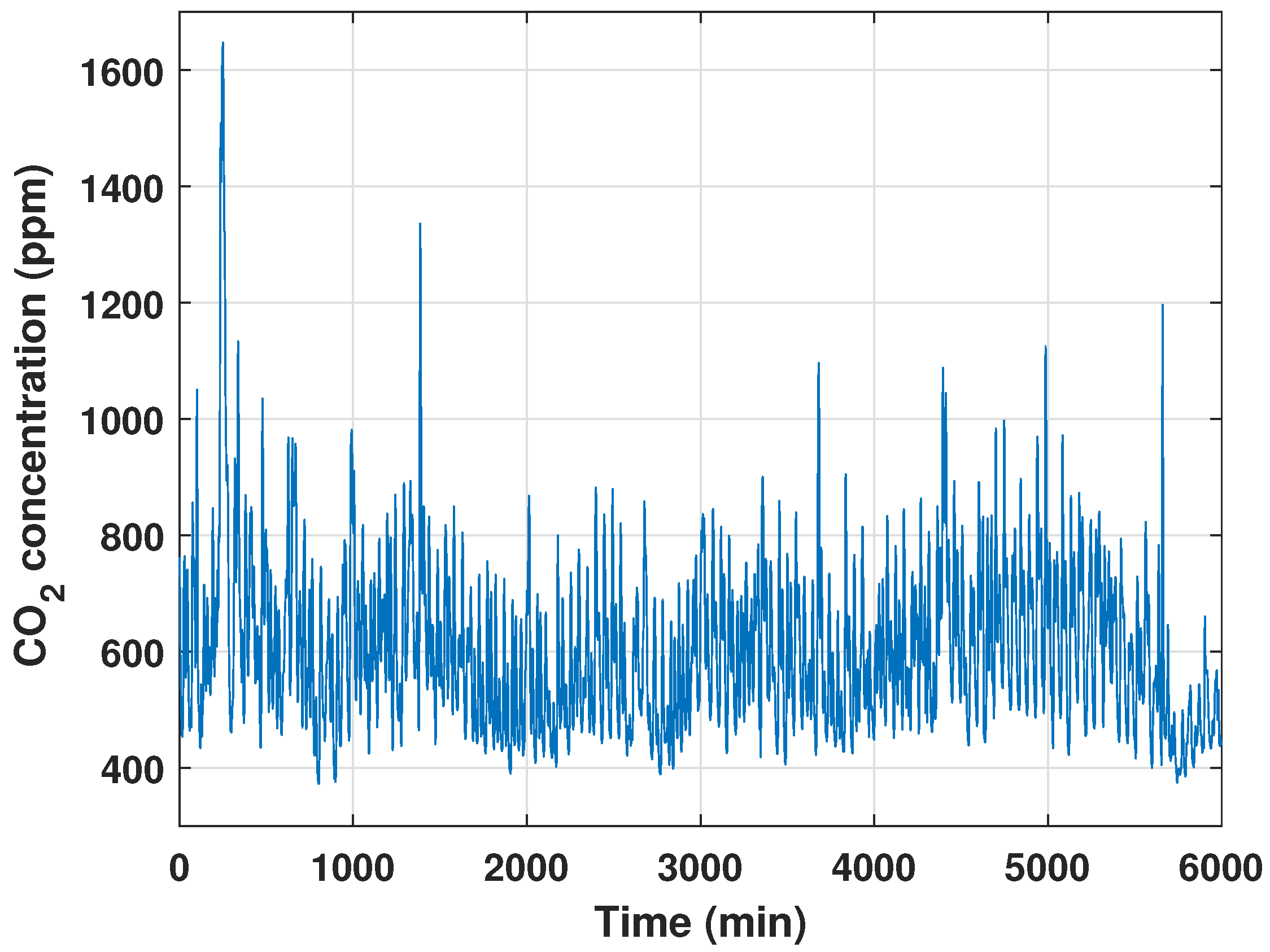
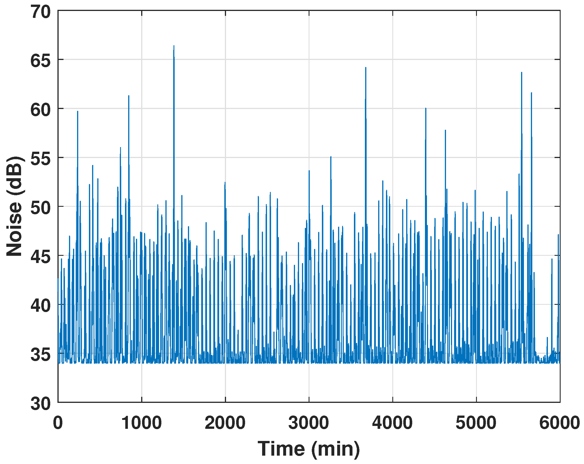
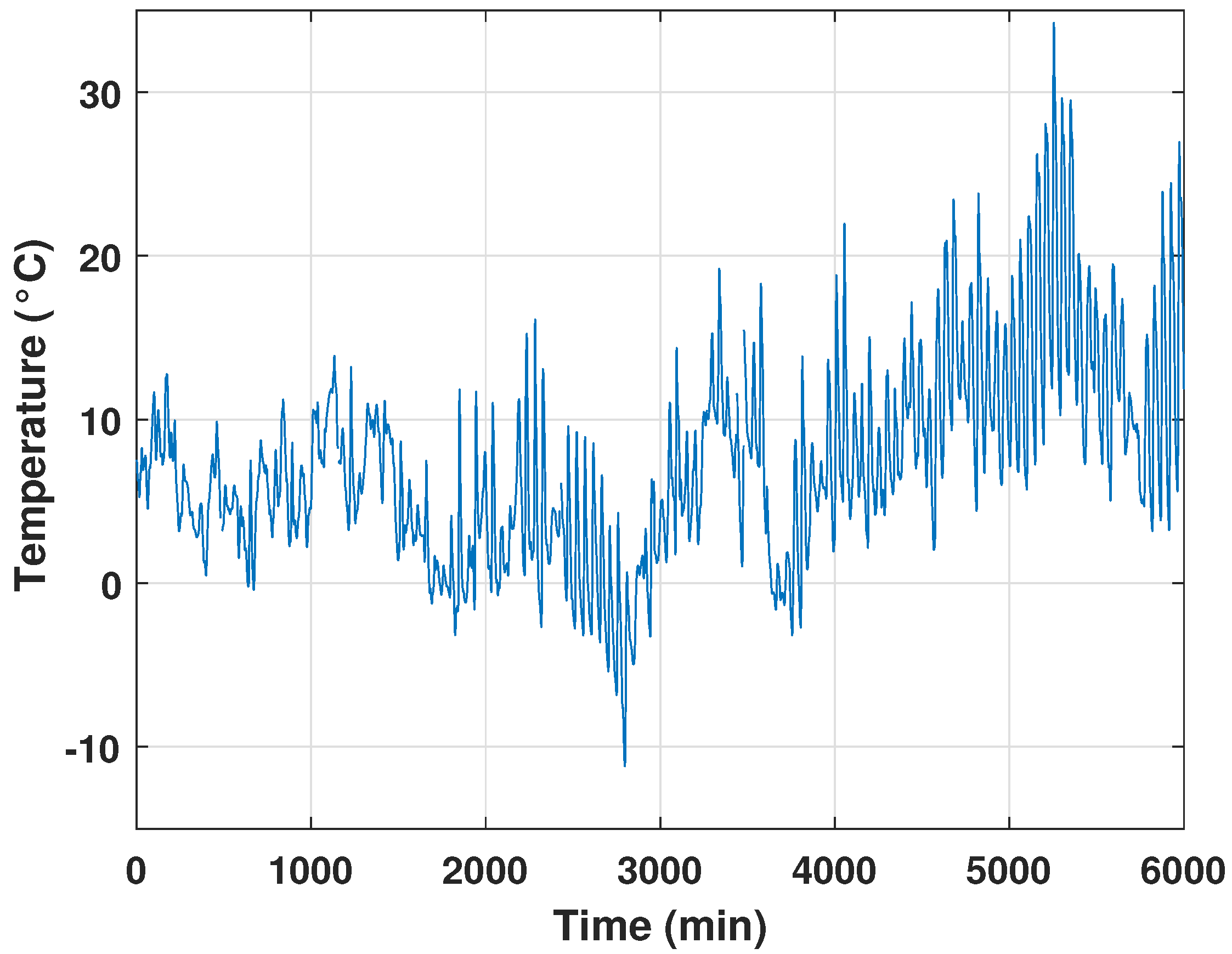
The concentration of these factors varied depending on the room; for example, the concentration of CO in the living room differed from that in the office or the kitchen. Moreover, the CO variable does not have a direct relationship with the interior temperature. However, because CO is a strong predictor of room occupancy, it may have a direct impact on the indoor temperature during the cold season. The variation in the CO, the noise, and the temperature are given by Figure 1, Figure 2 and Figure 3, respectively.
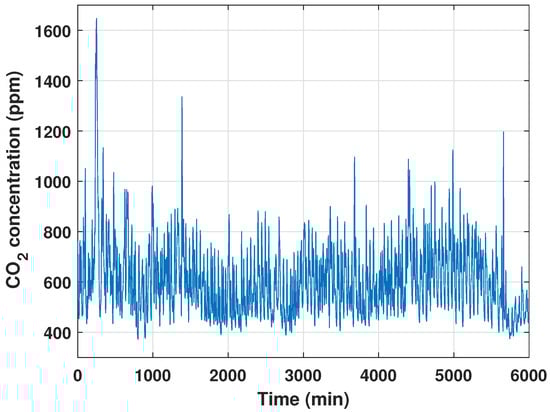
Figure 1.
Overview of the CO set points.
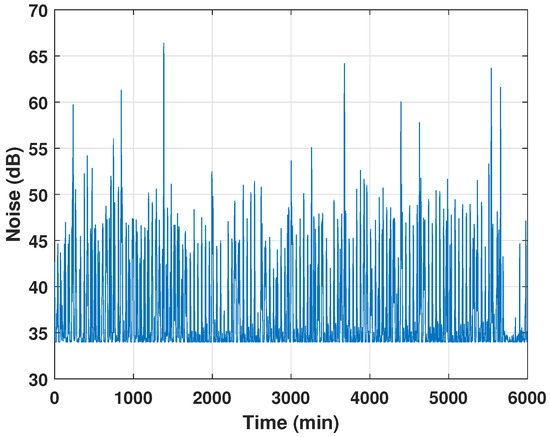
Figure 2.
Overview of the room noise set points.

Figure 3.
Overview of the room temperature set points.
3.2. Data Pre-Processing
The prediction of building energy use based on an occupant behavior assessment is a multivariate time series issue in which sensors create data that may contain uncertainty, redundancy, missing values, non-unified time intervals, noise, and so on. Traditional machine learning techniques struggle to reliably anticipate power usage due to unpredictable trend components and seasonal trends. The collection of suitable data contributes to efficiently addressing prediction challenges. As a result, several considerations should be made [20]. So, numerous techniques have been proposed to obtain meaningful inferences and insights; nevertheless, these solutions are still in the early phases of development. Therefore, current research is focusing on improving the procedures for processing and cleaning the collected data in order to produce accurate prediction [21].
3.2.1. Missing Values
Many real-world datasets may include missing values for various reasons. So, training a model using a dataset that has a large number of missing values can have a considerable influence on the machine learning model’s quality. To prevent information leakage, missing data were interpolated using Exponential Moving Average (EMA). This method is described in [22].
3.2.2. Normalisation
The data for a sequence prediction problem probably need to be normalised to the range of [−1, +1] when training a neural network such as a long short-term memory recurrent neural network. When a network is fit on unscaled data, it is possible for large inputs to slow down the learning and convergence of that network and, in some cases, prevent the network from effectively learning the problem. The Z-score is used for the normalization, and the formula is given as [23]:
where:
and n is the number of time periods.
4. Modeling Approaches
The main aim of this research is to investigate the performance of various occupancy forecasting strategies to identify the most accurate ones. In fact, we choose three distinct methods, based on a deep learning method: GA-LSTM and PSO-LSTM as optimiser based-models and LSTM as a simple deep learning technique.
4.1. LSTM Architecture
Recurrent Neural Networks (RNNs) struggle with learning long-term dependencies. LSTM-based models are an extension of RNNs that can solve the vanishing gradient problem and exploding gradient problem of RNNs and which perform more favorably than RNN on longer sequences. LSTM models basically expand the memory of RNNs to allow them to maintain and learn long-term input dependencies properly. This memory expansion can recall data for a longer amount of time, allowing them to read, write, and delete information from their memories. The LSTM memory is referred to as a “gate” structure because it has the power to decide whether to keep or discard memory information [24,25]. A gate is a way of transferring information selectively that includes a sigmoid neural network layer and a bitwise multiplication operations. The LSTM process and mathematical representation consists mostly of the four phases listed below [26]:
1. Deciding to remove useless information:
where represents the forget gate and is the sigmoid activation function and it can be defined as:
This function is utilized for this gate to decide what information should be removed from the LSTM’s memory. This decision is mainly dependent on the values of the previous hidden layer output and the input . The output takes a value between 0 and 1, where 0 means fully discard the learned value and 1 means preserve the entire value. is the recurrent weight matrix, while is the bias term.
2. Updating information:
in which is the input gate and denotes if the value needs to be updated or not and designates a vector of new candidate values that will be added into the LSTM memory. Indeed, the sigmoid layer determines which values require updating, and the tanh layer generates a vector of new candidate values.
3. Updating the cell status:
where and represent the current and previous memory states, respectively. This phase is carried out by updating the previous cell’s state, multiplying the old value by , deleting the information to be forgotten, and adding to generate a new candidate value.
4. Outputting information:
where is the output gate and is the current hidden layer outputs whose representations are a value between and 1. This step defines the ultimate result. To begin, a sigmoid layer, represented by , selects which part of the cell state will be output. The cell state is then processed by the tanh activation function and multiplied by the sigmoid layer output to create the output.
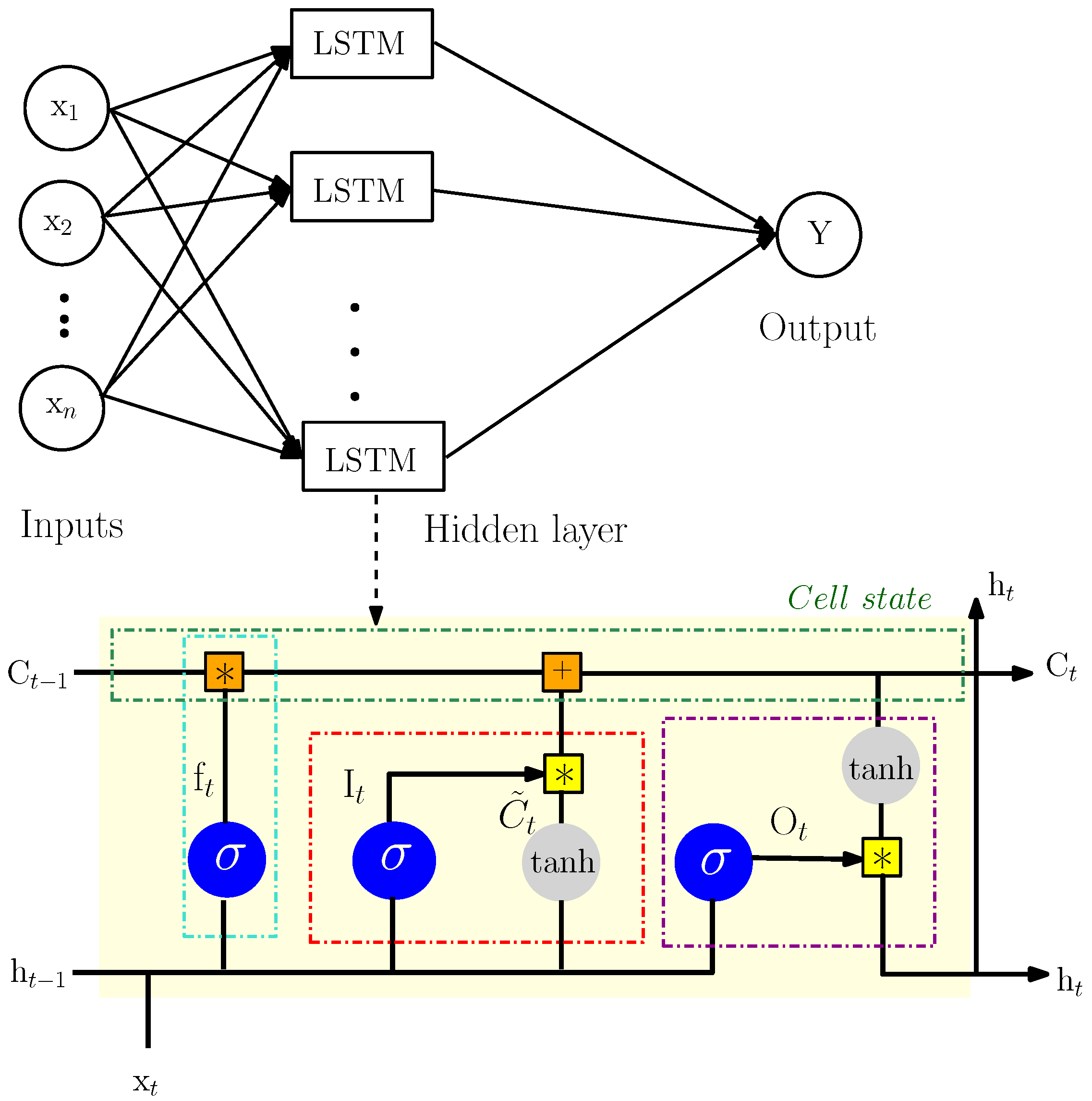
A typical LSTM network is seen in Figure 4. LSTM layers are composed of memory blocks rather than neurons. These memory blocks are interconnected across the layers, and each block may contain one or more recurrently connected memory elements or cells. As indicated in this figure (yellow shaded area), the flow of information is managed by three types of gates: the forget gate (), the input gate (), and the output gate ().
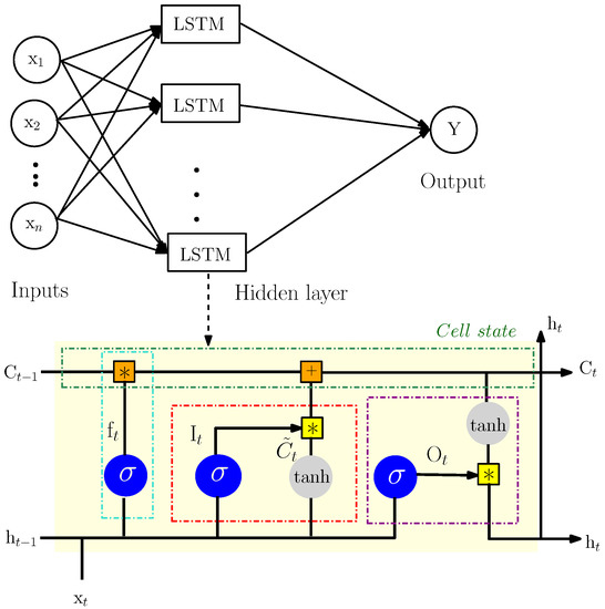
Figure 4.
A typical Long Short-Term Memory (LSTM) network topology.
4.2. LSTM Model Settings and Optimisation
Optimizing an LSTM model entails establishing a set of model parameters that yields the best model performance. The number of units and hidden layers and the optimiser, activation function, batch size, and learning rate are typical examples of such elements. So, the choice of a suitable algorithm is critical to success in addressing any type of optimisation issue. Wolpert and Macready demonstrated this in their “no free lunch” theorem, which states that no method is perfect for solving every type of optimisation issue. As a result, the basic idea is to select an effective optimisation approach to solve a given hand-in optimisation problem with less computational effort and a greater rate of convergence [27].
4.2.1. Genetic Algorithm (GA)
Genetic algorithms (GAs) have been around for over four decades. GAs are heuristic search algorithms that provide answers to optimisation and search problems. The name “GA” is derived from the biological terminology of natural selection, crossing, and mutation. In reality, GAs simulate natural evolutionary processes [28]. Thus, a literature review provides many instances of using GA in the analysis and optimisation of various elements from many sectors, such as energy systems. Moreover, GA can be used for the optimisation of ANN predictions or for the optimisation of ANN architecture [29]. GAs provide a general and global optimisation process. Since the GA is a global search technique, it will be less vulnerable to local search flaws such as back-propagation. The GA may be used to design the network’s architecture as well as its weight. There have been various attempts to utilise GAs to determine the architecture of a neural network and the link weights for a fixed architecture network. Many attempts have been made to use a GA to determine the architecture as well as the link weights.
4.2.2. Particle Swarm Optimization (PSO)
The particle swarm optimisation (PSO) method is a swarm-based stochastic optimisation approach introduced by Eberhart and Kennedy (1995). This technique replicates the social behavior of birds inside a flock to reach the food objective. A swarm of birds approaches their food goal using a combination of personal and communal experience. They constantly update their position based on their best position as well as the best position of the entire swarm, and reunite themselves to form an ideal configuration [30]. This nature-inspired method is becoming increasingly popular due to its reliability and easy implementation. In addition, classical neural networks do not operate well when forecasting parameters within short intervals. Moreover, because of their dependability, hybrid ANNs based on particle swarm optimisation have been frequently advocated in literature reviews. The PSO method, like the GA, is used as an optimisation technique within neural networks to optimise ANN forecasts or ANN architecture (the number of layers, neurons, etc.) [31]. Thus, we use this algorithm to optimise the weights.
4.3. LSTM Network Parameters
The network’s trainable parameters, known as the trainable weights, influence the network’s complexity. They are represented in LSTMs via connections between the input, hidden, and output layers, as well as internal connections. The following formula is used to calculate the Number of Trainable Weights (NTW) of a neural network with x inputs, y outputs, and z LSTM cells in the hidden layer:
where:
- -
- : the connection weights between the input layer and the hidden layer;
- -
- : the hidden layer’s recursive weights;
- -
- : the hidden layer’s bias;
- -
- : the connection weights between the hidden layer and the output layer;
- -
- y: the output layer’s bias.
Choosing ideal neural network settings can frequently imply the difference between mediocre and peak performance. However, there is limited information in the literature on the selection of different neural network parameters x, y, and z; it requires the expertise of professionals.
4.4. Train–Validation–Test dataset
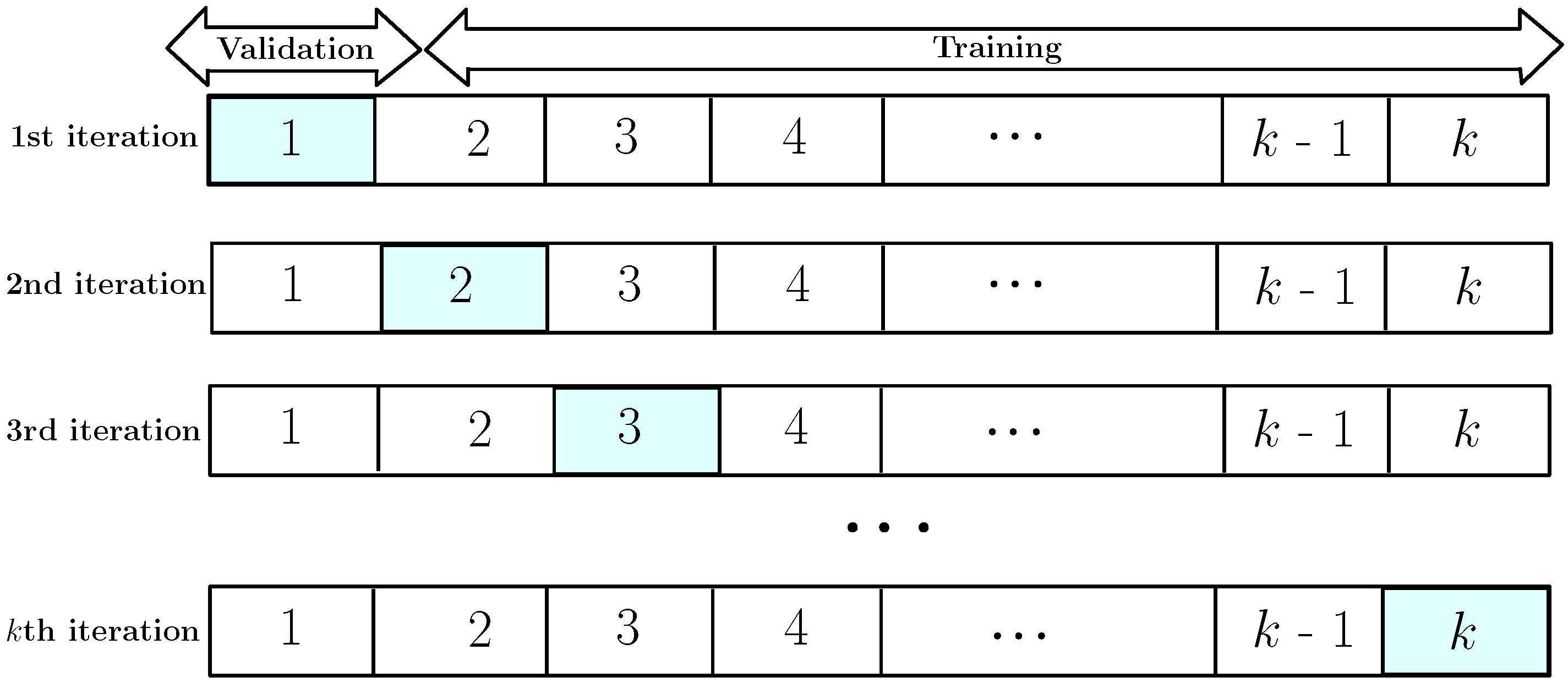
The one-year target variables were divided into three datasets: the first served as the training set, the second served as the test set, and depending on the length of the output sequence, random samples drawn from the last part served as the validation set. So, for the validation, we use cross-validation, which is a popular data resampling approach for estimating the true forecasting prediction error of models and tuning model parameters. This technique evaluates the generalization capabilities of prediction models and prevents over-fitting. It is the process of generating numerous train–test splits from the training data, which are then applied to adjust the model [32]. k-fold cross-validation is identical to repeated random sub-sampling, but the sampling is performed in such a manner that no two test sets overlap. The available learning set is divided into k disjoint subsets of about equivalent size. Indeed, each time, one of the k subsets is utilised as the validation/test batch, while the remaining (1) subsets are combined to form the training set. The total efficacy of the model is calculated by averaging the error estimation over all k trials. Each sample is placed in a validation/test set precisely once and in the training set (1) times [33]. Figure 5 illustrates this process as a popular evaluation mechanism in machine learning.
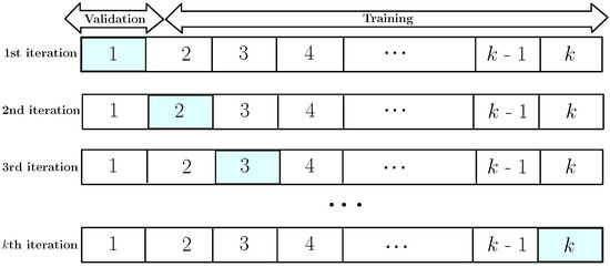
Figure 5.
k-fold cross-validation.
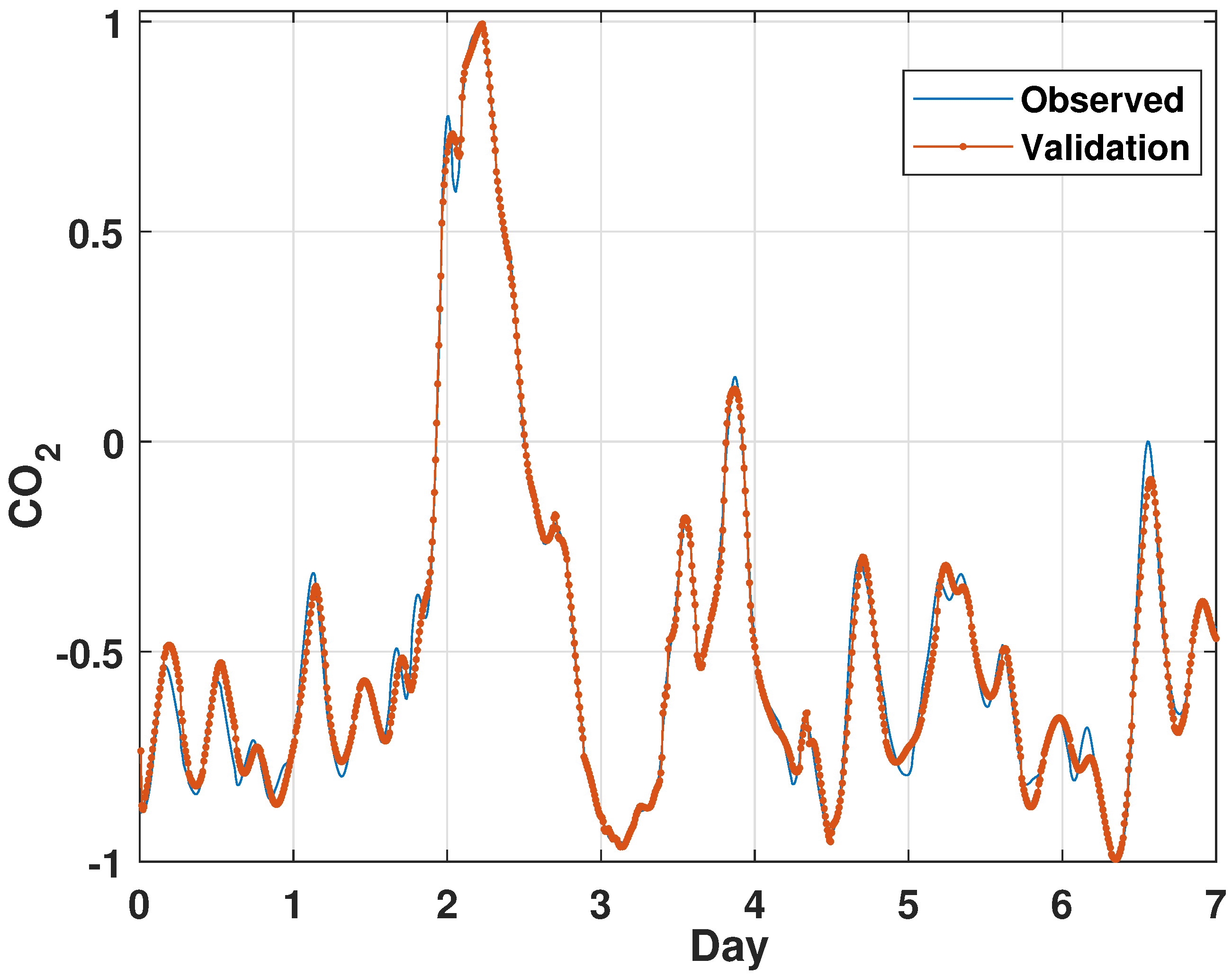
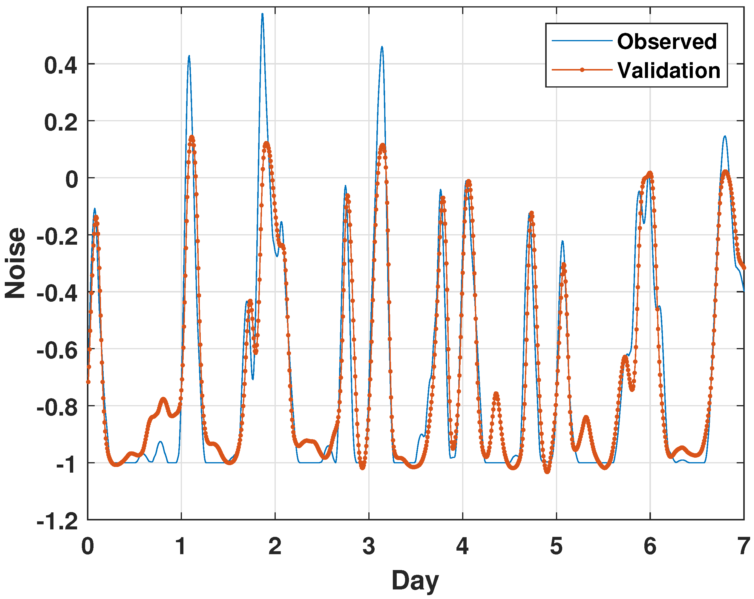
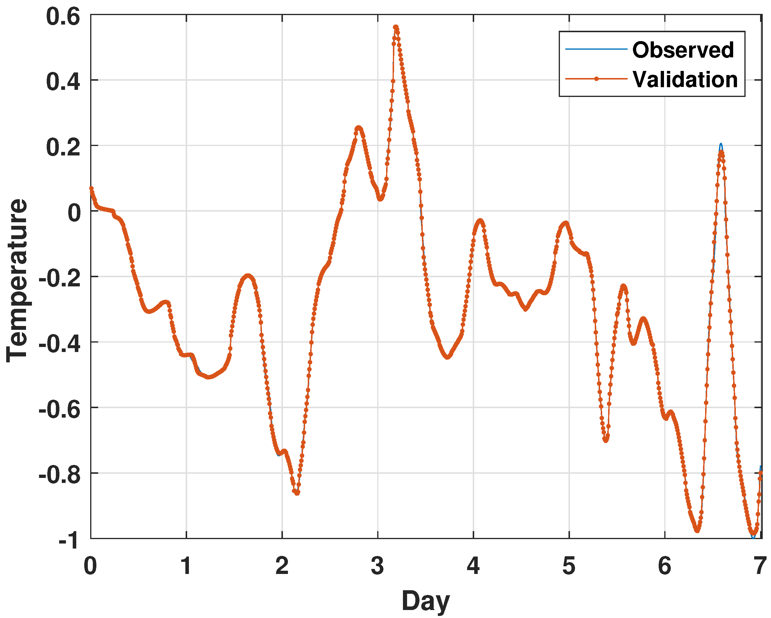
We train the LSTM with various architectures for 12-h forecasting of thermal parameters such as CO, noise, and temperature. As a result, the window size of the input and output parameters is determined by the time scale of the chosen parameter prediction. We apply the ADAM optimiser, which is one of the optimisation methods employed in deep learning. The learning rate is fixed to 0.01 and gradually drops after every 50 epochs. We train the LSTM with 60, 60, and 100 hidden units for the forecasting of the CO, the noise, and the temperature, respectively. The window size of the input and output parameters depends on the time scale of the load prediction. The validation and training results of each parameter are illustrated in Figure 6, Figure 7 and Figure 8.

Figure 6.
Training and validation of the CO data.
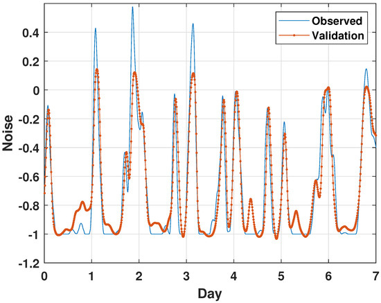
Figure 7.
Training and validation of the noise data.
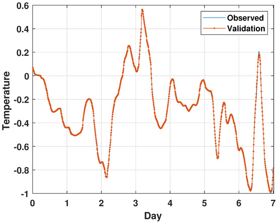
Figure 8.
Training and validation of the temperature data.
4.5. Evaluation Metrics
This study uses the Root Mean Square Error () as the loss function and the Mean Absolute Error () and the Correlation Coefficient () to evaluate the various performance measures. These indicators are measurements of the anticipated value’s departure from the actual data, and they indicate the prediction’s overall inaccuracy. The corresponding definition of each indicator is given by the following as [34]:
where and represent the real value and the forecasted value at the time t, N denotes the total time step, and and are the average of the real value and the forecasted value, respectively. The smaller the values of and , the smaller the deviation of the projected outcomes from the actual values. A value of closer to 1 indicates lower errors and a more accurate prediction.
5. Experimental Results
5.1. Parameters Forecasting
We show in this research a forecast of the thermal characteristics of a smart house outfitted with various types of sensors. The fundamental architecture of LSTM networks is predetermined and immutable; each LSTM unit has a vector input of n values, including the current value of the specified parameters (CO, noise, and temperature) at time as well as the past values. We create three neural networks with various designs, each one adapted to the predicting parameter. After 10 min, these neural networks can forecast. We can anticipate the full period of the required horizon by repeating the process and selecting the appropriate parameters for these models.
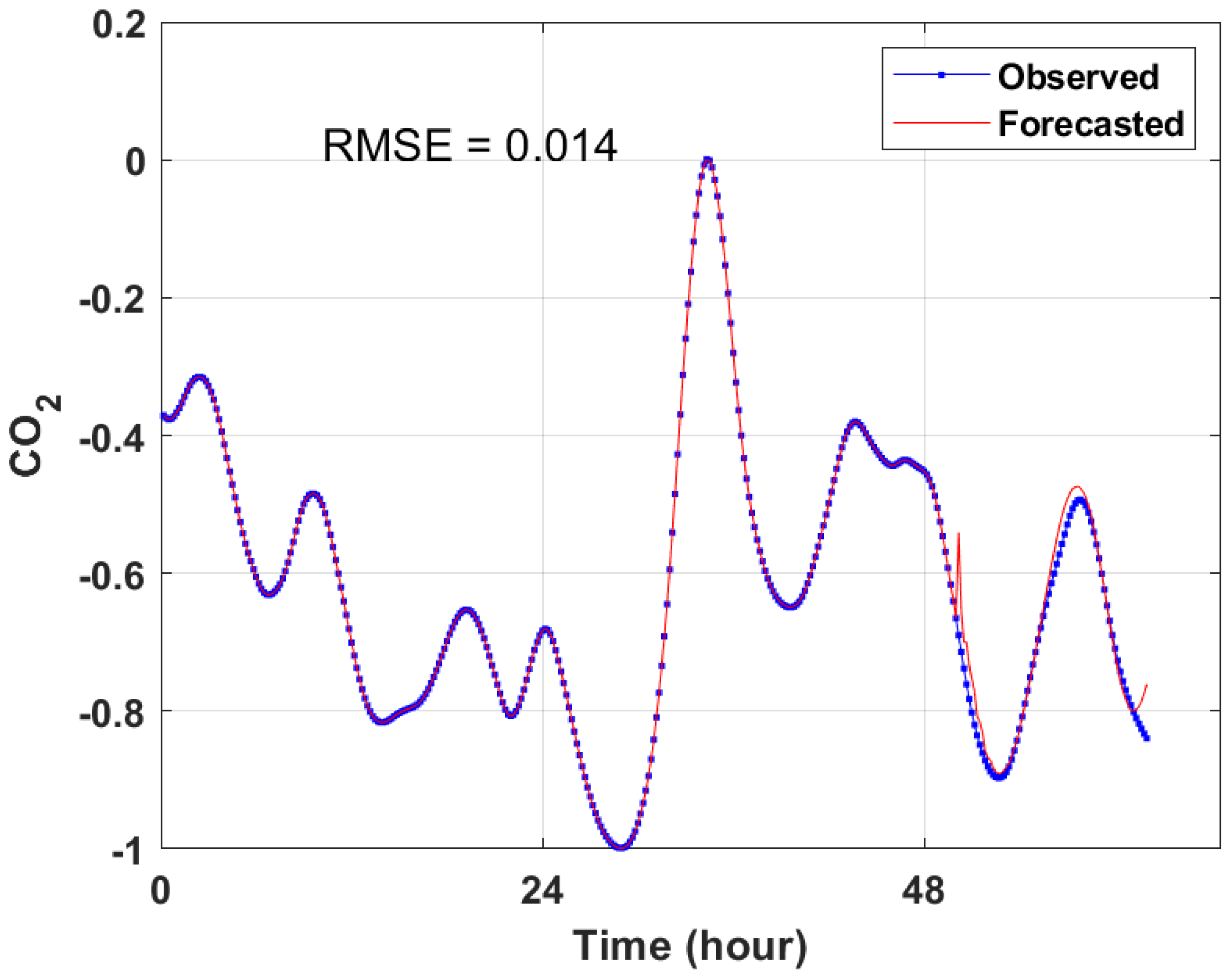
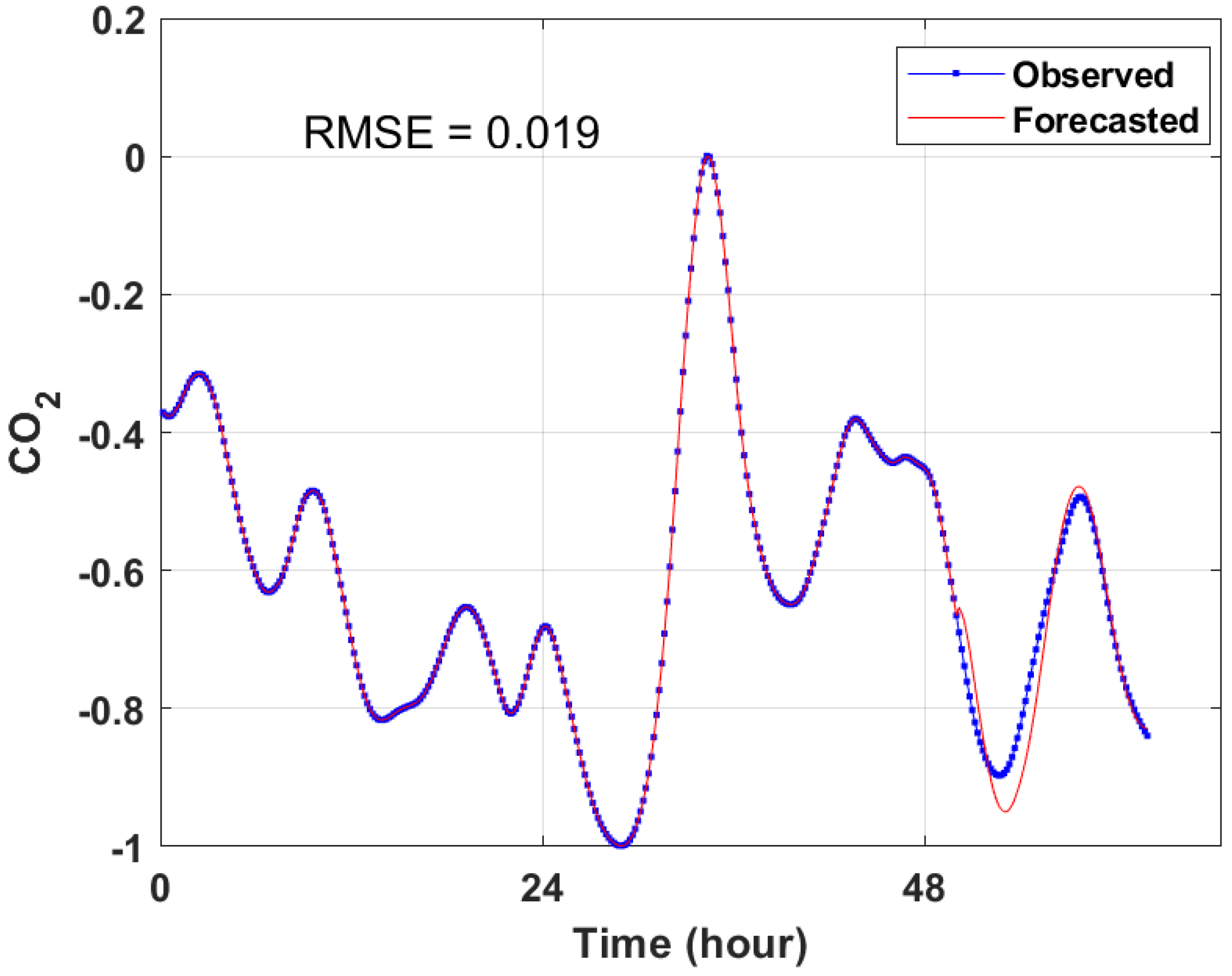
5.2. CO Forecasting
In the first experiment, we give the CO prediction of a house for 12 h. Figure 9, Figure 10 and Figure 11 show the predicted results obtained by the LSTM, the GA-LSTM, and the PSO-LSTM algorithms, respectively. As shown, the predicted results are closer to the real data values and the RMSE of each technique is quite low, which proves the forecasting performance of the suggested strategies.

Figure 9.
CO forecasting by LSTM.

Figure 10.
CO forecasting by GA-LSTM.

Figure 11.
CO forecasting by PSO-LSTM.
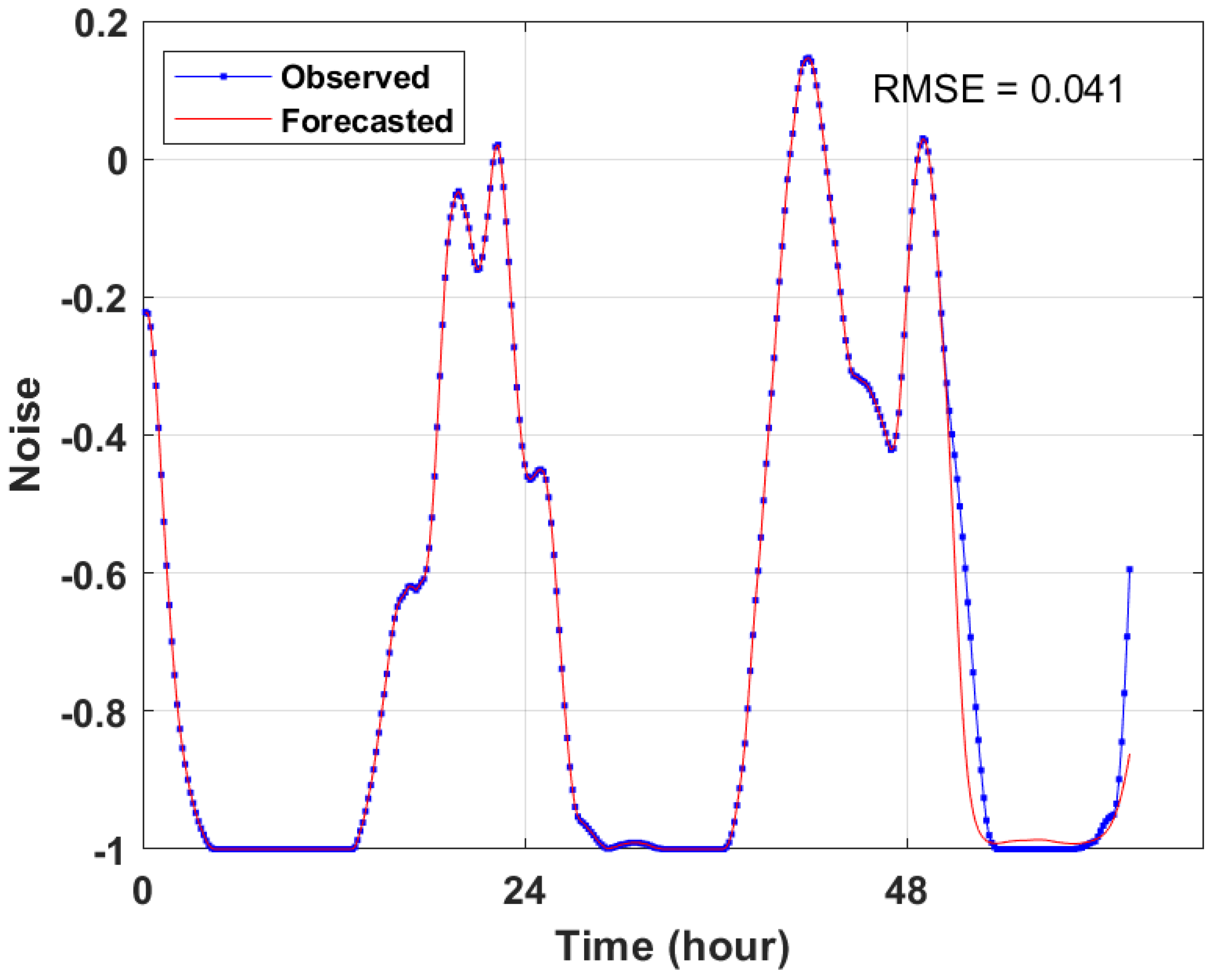
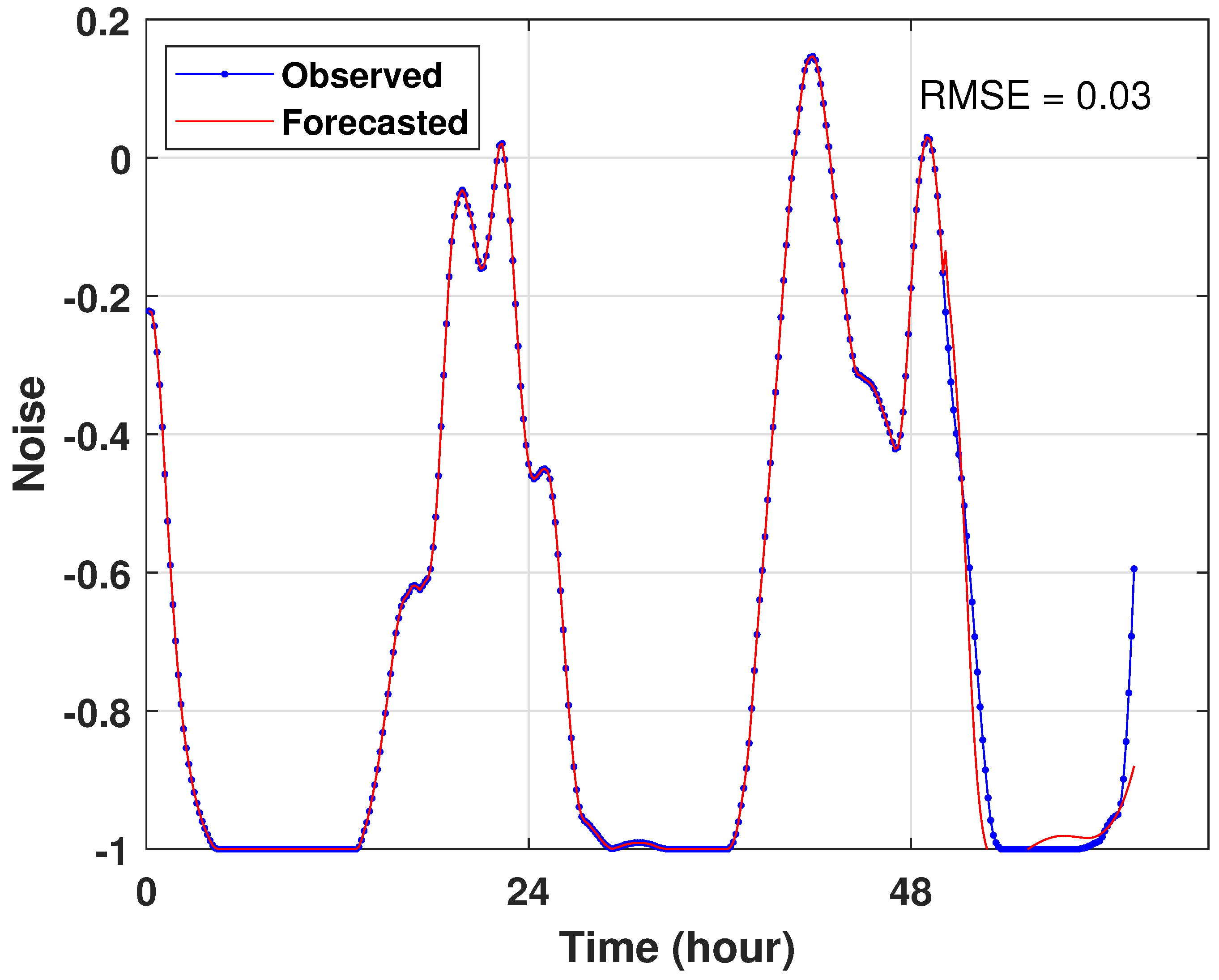
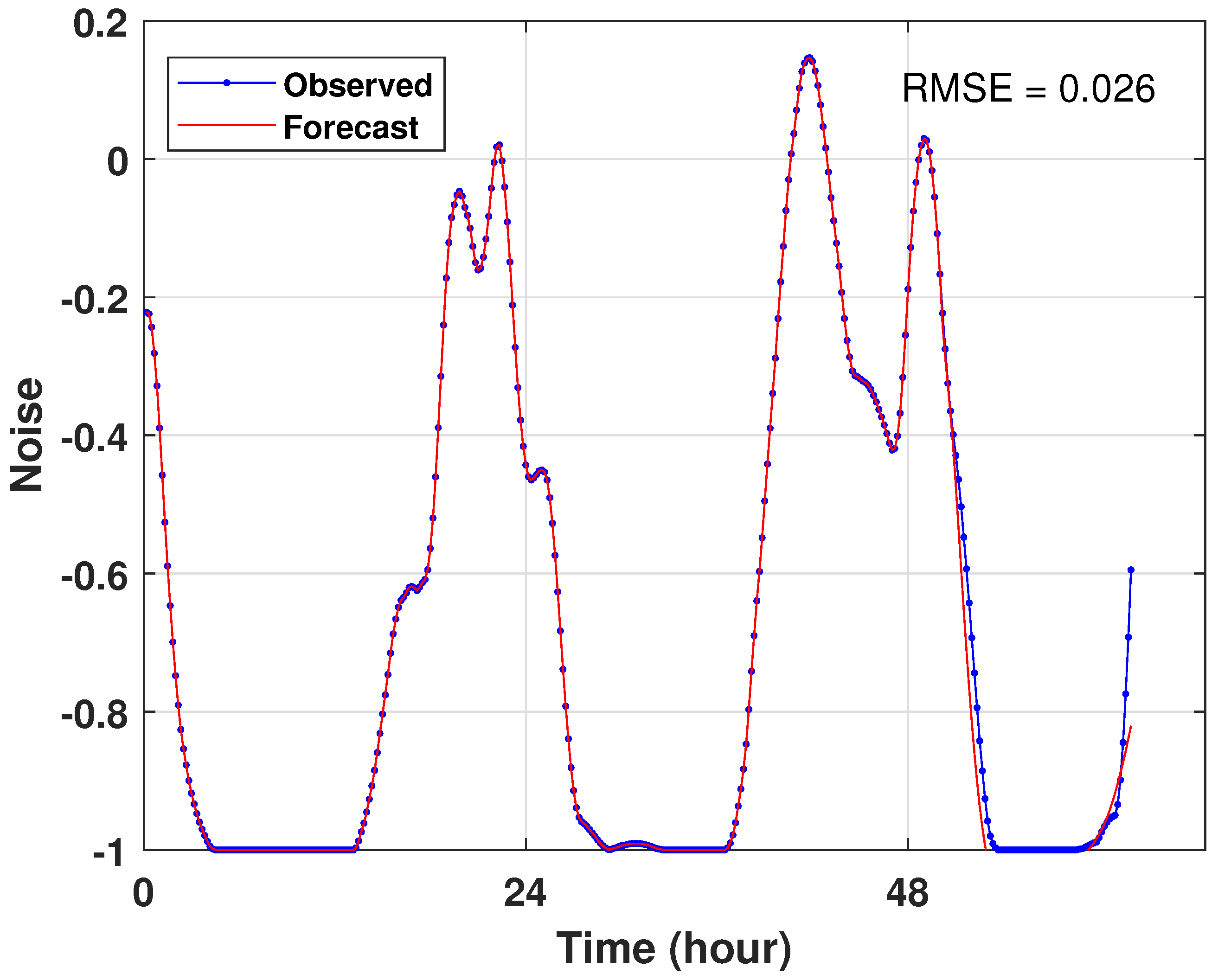
5.3. Noise Forecasting
The second experiment also illustrates the noise prediction results for 12 h. Figure 12, Figure 13 and Figure 14 show the findings with the error rate of the LSTM, the GA-LSTM, and the PSO-LSTM models. It appears that each model’s curve prediction retains the shape of the real data curve.
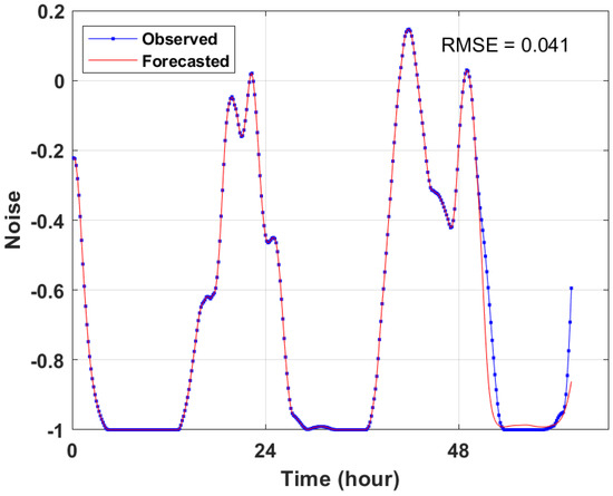
Figure 12.
Noise forecasting by LSTM.
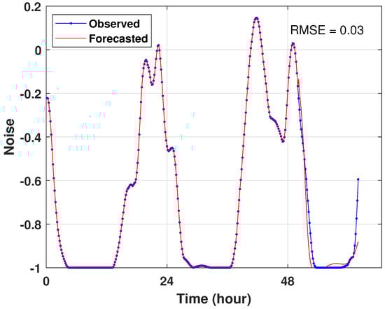
Figure 13.
Noise forecasting by GA-LSTM.
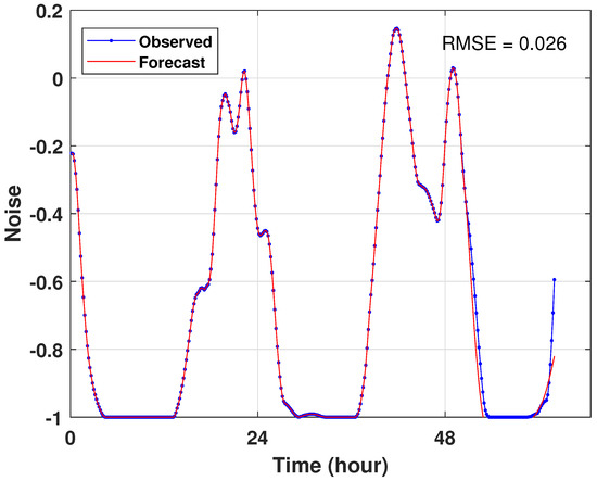
Figure 14.
Noise forecasting by PSO-LSTM.
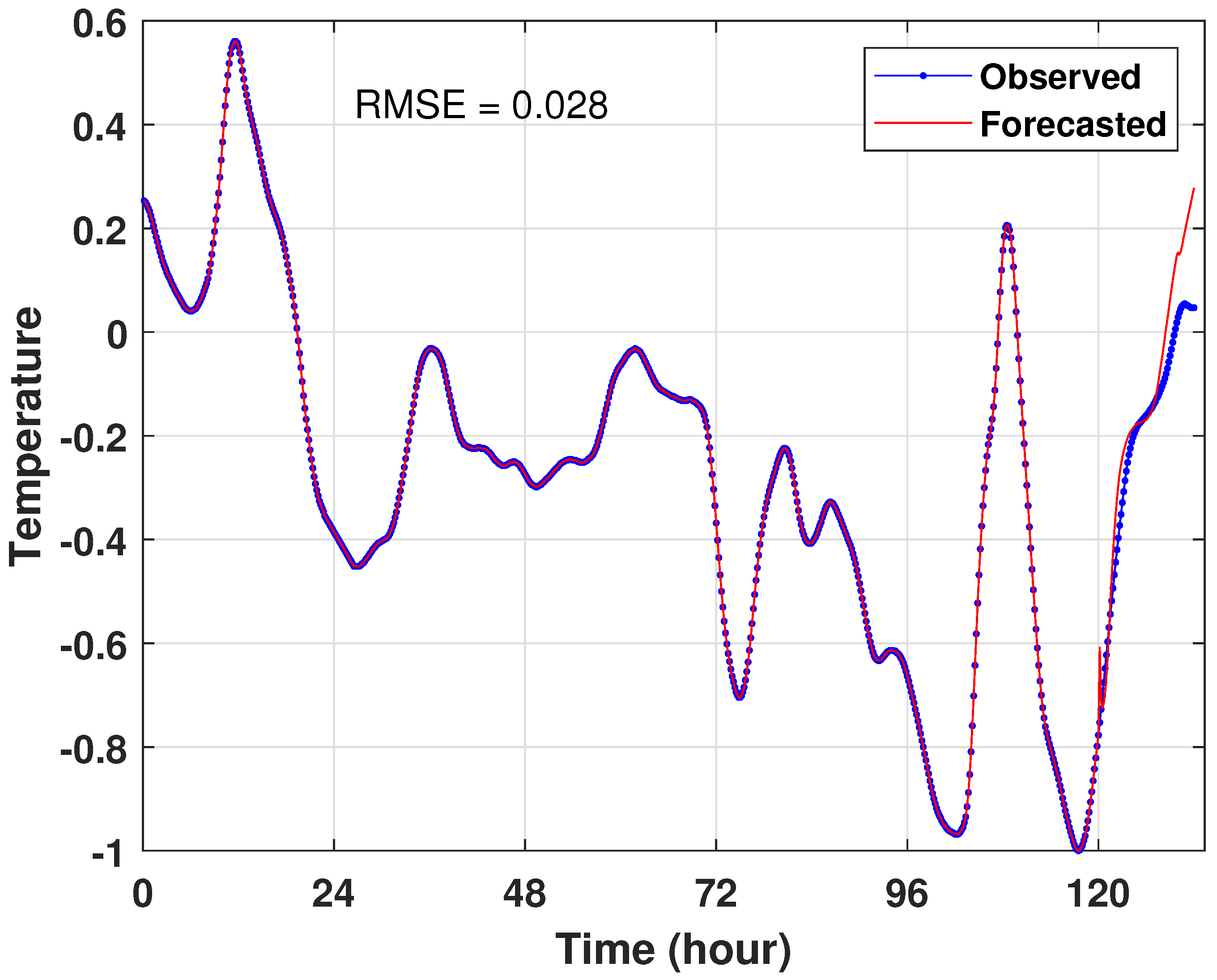
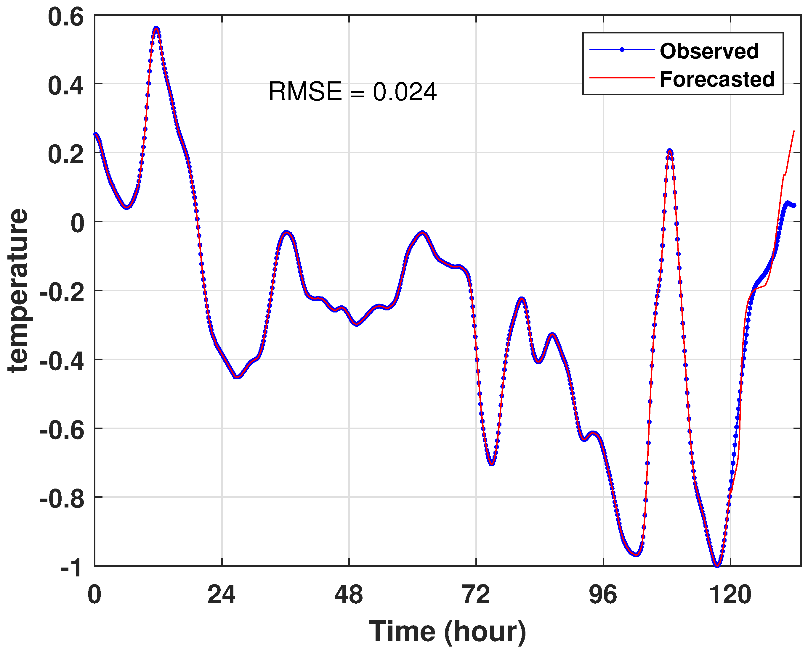
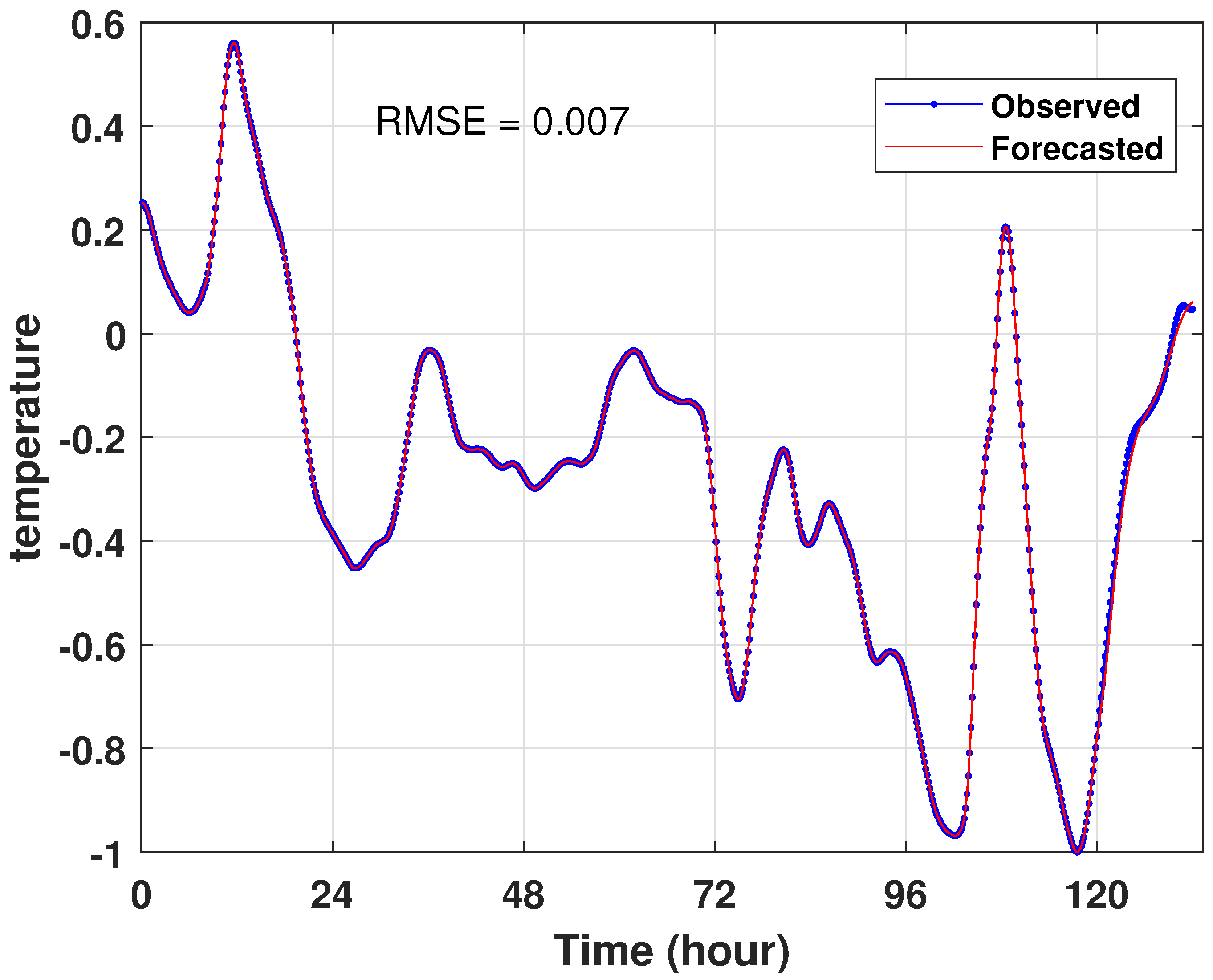
5.4. Temperature Forecasting
The third experiment shows the temperature forecasted results for 12 h. Figure 15, Figure 16 and Figure 17 depict the results with the RMSE value of the LSTM, the GA-LSTM, and the PSO-LSTM approaches. Likewise, each model’s curve prediction looks to keep the form of the real data curve.
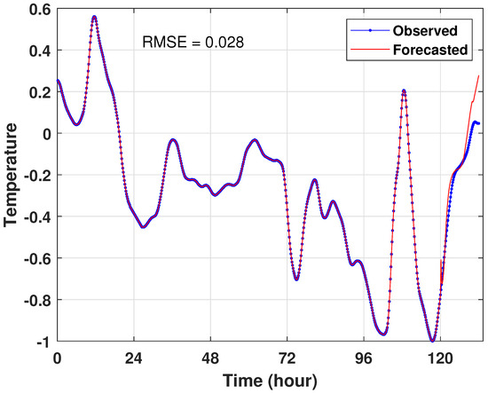
Figure 15.
Temperature forecasting by LSTM.
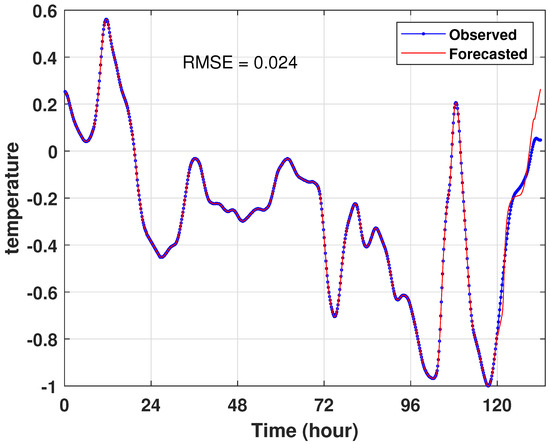
Figure 16.
Temperature forecasting by GA-LSTM.
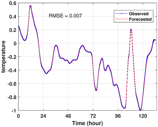
Figure 17.
Temperature forecasting by PSO-LSTM.
5.5. Analysis of Results
This work basically assesses the performance of the suggested model from two angles: precision and running time. Table 1, Table 2, and Table 3 provide the various performance measures for testing predictions on the studied building.

Table 1.
Performance criteria of the CO prediction.
Table 2.
Performance criteria of the noise prediction.
Table 3.
Performance criteria of the temperature prediction.
We can see that the implemented approaches produce quite excellent results, and the predicted findings are precise and dependable.
Table 1, Table 2 and Table 3 reveal that the two performance metrics, and , have small values. These predictions are fairly close and representative to the real data. The correlation coefficient () is also very close to 1, which proves the high precision of the forecasting strategies. As indicated in the tables and figures of forecasting results, the simple LSTM model without optimisation gives the worst results compared with the GA-LSTM and the PSO-LSTM techniques. We emphasize that the experimental results of the CO prediction show that the GA-LSTM outperforms the PSo-LSTM and the LSTM models with s of 0.0135, 0.0185, and 0.0281 and s of 99.80%, 99.62%, and 99.16% for GA-LSTM, PSO-LSTM, and LSTM, respectively. For noise and temperature prediction, the performance of the PSO-LSTM outperforms the GA-LSTM in terms of and . Overall, we have successfully shown that the proposed optimisation techniques (GA-LSTM and PSO-LSTM networks) may successfully extract relevant information from noisy human behavior data.
The statistical analysis of the obtained results shows that the proposed model tuned by the two evolutionary metaheuristic search algorithms (GA and PSO) provides more precise results than the benchmark LSTM model, whose parameters were established through limited experience and a discounted number of experiments.
6. Conclusions
In this work, we have proposed two optimised metaheuristic algorithms based on the LSTM architecture for dealing with occupancy forecasting in the context of smart buildings. The GA-LSTM and PSO-LSTM models give very satisfactory prediction results with a high level of precision and reliability compared with the LSTM forecasting results. The choice of these two methods (PSO and GA) is based on their reputation in literature. A comparison shows that the implementation of the two metaheuristic algorithms (GA and PSO) for the optimal configuration of occupancy forecasting derived an optimal LSTM model that performs significantly better than the benchmark models, including other machine learning approaches such as the basic LSTM model. The predicted values have been used to check the presence of residents and then control real electrical consumption. This was carried out to prove that the optimised LSTM can decrease power consumption, improve security, and maintain comfort for the occupants. A potential field for future research would be to perform thermal parameters forecasting, using recurrent neural networks, for various construction such as hospitals, hotels, and public establishments. It would be worthwhile to investigate whether a recurrent neural network can maintain such a high accuracy to forecast thermal features and room occupancy rates in a smart building. Thus, future studies will also focus on the deployment and integration of various hybrid optimisation algorithms in recurrent neural networks such as the LSTM model in order to select the best architecture, weights, and learning rate in order to achieve greater energy savings in the building energy management system. As a result, our findings provide a solid foundation for future research aimed at providing a more accurate assessment of building occupancy. Nonetheless, the current findings will provide a basis for occupancy prediction, which might be used to enhance our context-driven approaches for managing active building systems such as the HVAC, lighting, and shading systems. Again, a forecasting model for thermal characteristics and room occupancy rates with a low estimation error would help energy producers in making operational, tactical, and strategic decisions. Finally, better building load forecasting allows the implementation of the real-time management of smart buildings.
Author Contributions
Conceptualization, L.C.-A. and B.M.; methodology, S.M., B.M. and L.D.; software, S.M. and S.L.; validation, S.M. and L.C.-A.; formal analysis, L.D. and L.C.-A.; investigation, S.M. and S.L.; resources, B.M. and L.D.; data curation, B.M. and L.D.; writing—original draft preparation, S.M.; writing—review and editing, L.C.-A. and S.L.; visualization, S.M.; supervision, L.C.-A. and L.D.; project administration, B.M., L.D. and L.C.-A.; funding acquisition, B.M. All authors have read and agreed to the published version of the manuscript.
Funding
This research received no external funding.
Institutional Review Board Statement
Not applicable.
Informed Consent Statement
Not applicable.
Conflicts of Interest
The authors declare no conflict of interest.
References
- Stazi, F. Thermal Inertia in Energy Efficient Building Envelopes; Butterworth-Heinemann: Oxford, UK, 2017. [Google Scholar]
- Lotfabadi, P.; Hancer, P. A comparative study of traditional and contemporary building envelope construction techniques in terms of thermal comfort and energy efficiency in hot and humid climates. Sustainability 2019, 11, 3582. [Google Scholar] [CrossRef]
- Alawadi, S.; Mera, D.; Fernández-Delgado, M.; Alkhabbas, F.; Olsson, C.M.; Davidsson, P. A comparison of machine learning algorithms for forecasting indoor temperature in smart buildings. Energy Syst. 2020, 13, 1–17. [Google Scholar] [CrossRef]
- Dai, X.; Liu, J.; Zhang, X. A review of studies applying machine learning models to predict occupancy and window-opening behaviours in smart buildings. Energy Build. 2020, 223, 2020. [Google Scholar] [CrossRef]
- Boodi, A.; Beddiar, K.; Amirat, Y.; Benbouzid, M. Building Thermal-Network Models: A Comparative Analysis, Recommendations, and Perspectives. Energies 2022, 15, 1328. [Google Scholar] [CrossRef]
- Turley, C.; Jacoby, M.; Pavlak, G.; Henze, G. Development and evaluation of occupancy-aware HVAC control for residential building energy efficiency and occupant comfort. Energies 2020, 13, 5396. [Google Scholar] [CrossRef]
- Fotopoulou, E.; Zafeiropoulos, A.; Terroso-Saenz, F.; Simsek, U.; Gonzalez-Vidal, A.; Tsiolis, G.; Gouvas, P.; Liapis, P.; Fensel, A.; Skarmeta, A. Providing Personalized Energy Management and Awareness Services for Energy Efficiency in Smart Buildings. Sensors 2017, 17, 2054. [Google Scholar] [CrossRef]
- Hu, S.; Yan, D.; Guo, S.; Cui, Y.; Dong, B. A survey on energy consumption and energy usage behavior of households and residential building in urban China. Energy Build. 2017, 148, 366–378. [Google Scholar] [CrossRef]
- Cao, T.D.; Delahoche, L.; Marhic, B.; Masson, J.B. Occupancy Forecasting using two ARIMA Strategies. In Proceedings of the ITISE 2019, Granada, Spain, 25–27 September 2019; Volume 2. [Google Scholar]
- Mariano-Hernández, D.; Hernández-Callejo, L.; García, F.S.; Duque-Perez, O.; Zorita-Lamadrid, A.L. A review of energy consumption forecasting in smart buildings: Methods, input variables, forecasting horizon and metrics. Appl. Sci. 2020, 10, 8323. [Google Scholar] [CrossRef]
- Scheurer, S.; Tedesco, S.; Brown, K.N.; O’Flynn, B. Using domain knowledge for interpretable and competitive multi-class human activity recognition. Sensors 2020, 20, 1208. [Google Scholar] [CrossRef]
- Fang, Z.; Crimier, N.; Scanu, L.; Midelet, A.; Alyafi, A.; Delinchant, B. Multi-zone indoor temperature prediction with LSTM-based sequence to sequence model. Energy Build. 2021, 245, 111053. [Google Scholar] [CrossRef]
- Kaligambe, A.; Fujita, G.; Keisuke, T. Estimation of Unmeasured Room Temperature, Relative Humidity, and CO2 Concentrations for a Smart Building Using Machine Learning and Exploratory Data Analysis. Energies 2022, 15, 4213. [Google Scholar] [CrossRef]
- Massana, J.; Pous, C.; Burgas, L.; Melendez, J.; Colomer, J. Short-term load forecasting for non-residential buildings contrasting artificial occupancy attributes. Energy Build. 2016, 130, 519–531. [Google Scholar] [CrossRef]
- Zhao, J.; Liu, X. A hybrid method of dynamic cooling and heating load forecasting for office buildings based on artificial intelligence and regression analysis. Energy Build. 2018, 174, 293–308. [Google Scholar] [CrossRef]
- Bouktif, S.; Fiaz, A.; Ouni, A.; Serhani, M.A. Optimal deep learning lstm model for electric load forecasting using feature selection and genetic algorithm: Comparison with machine learning approaches. Energies 2018, 11, 1636. [Google Scholar] [CrossRef]
- Alawadi, S.; Mera, D.; Fernandez-Delgado, M.; Taboada, J.A. Comparative study of artificial neural network models for forecasting the indoor temperature in smart buildings. In International Conference on Smart Cities; Springer: Cham, Switzerland, 2017; pp. 29–38. [Google Scholar]
- Aliberti, A.; Bottaccioli, L.; Macii, E.; Di Cataldo, S.; Acquaviva, A.; Patti, E. A non-linear autoregressive model for indoor air-temperature predictions in smart buildings. Electronics 2019, 8, 979. [Google Scholar] [CrossRef]
- Zhu, J.; Yang, Z.; Mourshed, M.; Guo, Y.; Zhou, Y.; Chang, Y.; Wei, Y.; Feng, S. Electric Vehicle Charging Load Forecasting: A Comparative Study of Deep Learning Approaches. Energies 2019, 12, 2692. [Google Scholar] [CrossRef]
- Liu, Z.; Wu, D.; Liu, Y.; Han, Z.; Lun, L.; Gao, J.; Jin, G.; Cao, G. Accuracy analyses and model comparison of machine learning adopted in building energy consumption prediction. Energy Explor. Exploit. 2019, 37, 1426–1451. [Google Scholar] [CrossRef]
- Saleem, T.J.; Chishti, M.A. Data analytics in the Internet of Things: A survey. Scalable Comput. Pract. Exp. 2019, 20, 607–630. [Google Scholar] [CrossRef]
- Mahjoub, S.; Chrifi-Alaoui, L.; Marhic, B.; Delahoche, L. Predicting Energy Consumption Using LSTM, Multi-Layer GRU and Drop-GRU Neural Networks. Sensors 2022, 22, 4062. [Google Scholar] [CrossRef]
- Mahjoub, S.; Chrifi-Alaoui, L.; Marhic, B.; Delahoche, L.; Masson, J.B.; Derbel, N. Prediction of energy consumption based on LSTM Artificial Neural Network. In Proceedings of the 2022 19th International Multi-Conference on Systems, Signals Devices (SSD), Setif, Algeria, 6–10 May 2022; pp. 521–526. [Google Scholar]
- Siami-Namini, S.; Tavakoli, N.; Namin, A.S. The performance of LSTM and BiLSTM in forecasting time series. In Proceedings of the 2019 IEEE International Conference on Big Data (Big Data), Los Angeles, CA, USA, 9–12 December 2019; pp. 3285–3292. [Google Scholar]
- Apaydin, H.; Feizi, H.; Sattari, M.T.; Colak, M.S.; Shamshirband, S.; Chau, K.W. Comparative analysis of recurrent neural network architectures for reservoir inflow forecasting. Water 2020, 12, 1500. [Google Scholar] [CrossRef]
- Zhang, X.; Zhao, M.; Dong, R. Time-series prediction of environmental noise for urban IoT based on long short-term memory recurrent neural network. Appl. Sci. 2020, 10, 1144. [Google Scholar] [CrossRef]
- Jain, M.; Saihjpal, V.; Singh, N.; Singh, S.B. An Overview of Variants and Advancements of PSO Algorithm. Appl. Sci. 2022, 12, 8392. [Google Scholar] [CrossRef]
- Hoschel, K.; Lakshminarayanan, V. Genetic algorithms for lens design: A review. J. Opt. 2019, 48, 134–144. [Google Scholar] [CrossRef]
- Lorencin, I.; Andelic, N.; Mrzljak, V.; Car, Z. Genetic algorithm approach to design of multi-layer perceptron for combined cycle power plant electrical power output estimation. Energies 2019, 12, 4352. [Google Scholar] [CrossRef]
- Wang, D.; Tan, D.; Liu, L. Particle swarm optimization algorithm: An overview. Soft Comput. 2018, 22, 387–408. [Google Scholar] [CrossRef]
- Aljanad, A.; Tan, N.M.; Agelidis, V.G.; Shareef, H. Neural network approach for global solar irradiance prediction at extremely short-time-intervals using particle swarm optimization algorithm. Energies 2021, 14, 1213. [Google Scholar] [CrossRef]
- Berrar, D. Cross-validation. In Encyclopedia of Bioinformatics and Computational Biology; Elsevier: Amsterdam, The Netherlands, 2019; Volume 1, pp. 542–545. [Google Scholar] [CrossRef]
- Xiong, Z.; Cui, Y.; Liu, Z.; Zhao, Y.; Hu, M.; Hu, J. Evaluating explorative prediction power of machine learning algorithms for materials discovery using k-fold forward cross-validation. Comput. Mater. Sci. 2020, 171, 109203. [Google Scholar] [CrossRef]
- Xiao, Y.; Yin, H.; Zhang, Y.; Qi, H.; Zhang, Y.; Liu, Z. A dual-stage attention-based Conv-LSTM network for spatio-temporal correlation and multivariate time series prediction. Int. J. Intell. Syst. 2021, 36, 2036–2057. [Google Scholar] [CrossRef]

Disclaimer/Publisher’s Note: The statements, opinions and data contained in all publications are solely those of the individual author(s) and contributor(s) and not of MDPI and/or the editor(s). MDPI and/or the editor(s) disclaim responsibility for any injury to people or property resulting from any ideas, methods, instructions or products referred to in the content. |
© 2023 by the authors. Licensee MDPI, Basel, Switzerland. This article is an open access article distributed under the terms and conditions of the Creative Commons Attribution (CC BY) license (https://creativecommons.org/licenses/by/4.0/).