Six Days Ahead Forecasting of Energy Production of Small Behind-the-Meter Solar Sites

Abstract

Due to the growing penetration of behind-the-meter (BTM) photovoltaic (PV) installations, accurate solar energy forecasts are required for a reliable economic energy system operation. A new hybrid methodology is proposed in this paper with a sequence of one-step ahead models to accumulate 144 h for a small-scale BTM PV site. Three groups of models with different inputs are developed to cover 6 days of forecasting horizon, with each group trained for each hour of the above zero irradiance. In addition, a novel dataset preselection is proposed, and neighboring solar farms’ power predictions are used as a feature to boost the accuracy of the model. Two techniques are selected: XGBoost and CatBoost. An extensive assessment for 1 year is conducted to evaluate the proposed method. Numerical results highlight that training the models with the previous, current, and 1 month ahead from the previous year referenced by the target month can improve the model’s accuracy. Finally, when solar energy predictions from neighboring solar farms are incorporated, this further increases the overall forecast accuracy. The proposed method is compared with the complete-history persistence ensemble (CH-PeEn) model as a benchmark.

1. Introduction

A deployment of 138 GW of rooftop photovoltaic (PV) systems has been identified between 2020 and 2021 [1]. PV systems deployment did not slow down even during the COVID-19 pandemic and all of the related health and logistic limitations. The growth of behind-the-meter (BTM) solar sites makes net demand forecasting challenging as it introduces additional uncertainty in net demand patterns [2]. Net demand is the critical input in both short-term and long-term planning of power systems [3]. To carry this out, net demand must be forecasted, accounting for a modified shape pattern between the morning hours of the day and the end of the afternoon [4]. Net demand can be predicted directly or indirectly by subtracting the BTM PV power forecast from the demand. Therefore, forecasting models with enhanced accuracy for small BTM PV sites are important to support net demand forecasting in power systems.

One-step ahead forecasters were the most common between 2010 and 2019, while more recently, multi-step forecast methods are gaining momentum [5]. Even though many hybrid approaches have been proposed in the literature, they are limited mainly by intra-day horizons or, in some cases, limited to 3 days ahead [5]. For example, in [6], a hybrid method called physical hybrid artificial neural network (PHANN) is proposed to predict up to 72 h ahead. Finally, in [7], a hybrid method with artificial neural network (ANN) and an analog ensemble (AnEn) is proposed to generate 72 h forecasts of power.

In the solar energy forecasting domain, there are two primary training practices. The first approach, Generalization, is when research works use a significant amount of data as possible to train a unique model to forecast any hour of the day, month, or season. The second approach, Classification, is when different models are built based on categories. For example, the first two full years of data were used for training in [8], and in [9], the authors used the total accumulated historical data to train a model. On the other hand, an optimization using a selection training dataset with a standard setting consisting of days with different cloud conditions from half a year of data was applied in [10]. Whereas, in [11], three models were trained with a dataset divided into three categories: Sunny, cloudy, and overcast days, according to the mean irradiance.

The spatio-temporal correlation is attracting attention in solar energy forecasts. Some works have applied historical data from neighboring solar sites and weather stations to forecast solar energy. For example, five nearby solar irradiance stations, with distances from 0 to 200 km to predict from 5 min to 24 h ahead; first, solar irradiance, converted to solar power, was accounted in [12]. More recently, in [13], the authors considered the collaborative data from 44 rooftop-scale solar units located in a Portuguese city in their model to produce 6 h ahead of solar power forecasts.

In distinction to the common practices, we propose a new hybrid methodology with three groups of models and different inputs to cover a forecasting horizon of 6 days. Each group is trained for each hour of above zero irradiance. In addition, the method includes a monthly pattern preselection approach where the most recent and the most likely future weather patterns are present. We select similar months based on the target month we want to predict, reducing the available dataset to only the months with very similar characteristics to the target month. Namely, the previous month, the current month, and the next month ahead from the previous year are selected and referenced by the forecasting origin. This strategy balances enough generalization and similar days classification in a reduced dataset which is more correlated with the target forecast. Moreover, we propose the reinforcement of the methodology by benefiting from spatio-temporal correlation using publicly available regional aggregated solar power predictions (RASPP) as a feature. This specific feature helps the proposed method to take advantage of other forecasts for solar energy generation within the same neighboring region.

In summary, the main contributions of this work are as follows: First, we propose a horizontally cascaded set of models to extend the forecasting horizon of short-term solar energy forecasting to 6 days. The forecasting horizon of 6 days is divided into three groups of models with different inputs, and, within each group, a separate model for each hour of the day is proposed. Moreover, a novel classification and training strategy is proposed for the enhancement of forecast accuracy. Second, we propose the use of publicly available regional aggregated solar power predictions (RASPP) as an input to the model to benefit from potential spatio-temporal correlations between the power production at the target site and the general solar energy production patterns in the same geographical region.

The remainder of this paper is organized according to the following sections: Section 2 presents a literature review of solar power forecasting. Section 3 describes the proposed solar power forecasting methodology. Section 4 presents the numerical results and discussions, followed by Section 5, which summarizes this work, and suggests directions for potential future work.

2. Literature Review

The solar energy forecasting literature can be classified into subdomains regarding the spatial horizon [14], time horizon [15], methods [5], techniques [14], inputs [14], benchmarks [16], and level of uncertainty [17,18]. Regarding methods, some strategies consider numerical and probabilistic methods, physical models, and artificial intelligence (AI) techniques, including machine learning (ML), deep learning (DL), and hybrid methods [5]. In terms of time horizon [14], these works can be categorized into four subdomains: Intra-hour or nowcasting, intra-day, i.e., 6 h to day-ahead, or multi-days ahead or more prolonged (2 days and longer). Regarding modelling inputs [14], forecasting strategies consider endogenous inputs [8] and [19], exogenous, or both [20], including numerical weather predictions (NWP), sky cameras [17], satellite imagery [21], neighboring PV plants [22], adjacent weather stations [12], and other predictions.

A review of the literature showed that some works used a significant amount of data as possible to train a model. They based their models on Generalization. For example, in [8], where the first two full years of data were used for training; or in [9], the authors used the total accumulated historical data to train a model with no specific selection of days; and in [23], the authors used one whole year of data to train six models. However, in terms of Classification, different models are built based on categories. Some works targeted the pattern of the preselected data to train a model in order to focus on the similar pattern to be predicted, as seen in [10], in which an optimization using a selection training dataset with a standard setting consisting of days with different cloud conditions from half a year of data was applied; or in [11], the authors trained three models with the dataset divided into three categories: Sunny, cloudy, and overcast days, according to the mean irradiance; or in [24], the researchers developed a weather scenario based on generation, in which a copula was adopted to model the correlation among weather variables, including the data from local weather stations and historical NWP, through a high-dimensional joint distribution; or in [25], three selection methods were presented for training purposes: First, the previous 30 days, or second, the 30 days according to the absolute difference between the clearness index of the day to be predicted and each day included in the database, or finally the third strategy, which considered the 30 days according to the similarity between the empirical distribution function of the irradiance forecast for the day to be predicted and for each day included in the database. The first group of works considered that a generalization strategy would assist in increasing the quality of their models. On the other hand, the second group argued that a classification strategy would perform better. It is very unlikely that a model trained with data from Winter would be helpful to predict something during Summer. Therefore, we understand that a generalization strategy is ineffective in this case. Meanwhile, the second group relied on the forecasted weather in order to select the respective model to predict accurately. However, if the weather forecast is wrong, it is very likely that the prediction, based on the classified day would not perform well. For example, an overcast day would be predicted, but no clouds are above the solar panels and then, an underestimated production would be expected. In this case, a methodology that considers enough generalization and classification is needed. Therefore, a reduced dataset also divided by each hour of the day is a potential solution. In conclusion, to the best of our knowledge, the gap related to the month pattern preselection exists. As a result, it merits investigation in this paper.

Some works have explored the application of using historical data from neighboring solar sites or weather stations in the context of solar energy forecasting. For example, the authors of [26] accounted for 80 distributed rooftop PV plants in the Arizona region as a network of irradiance sensors to predict cloud speed and solar power; or the authors of [27] used historical information from five neighboring rooftop PV plants in the Netherlands and one meteorological station to predict solar power of a 500 W PV system; or the authors of [12] accounted for five nearby solar irradiance stations, with distances from 0 to 200 km for prediction, first, of solar irradiance, and then conversion to solar power; or the authors of [22] developed an individual model for each hour for each of three utility-scale solar farms (Solar Farms A, B, and C) to predict with an hourly resolution, accounting for the inclusion of independent variables from the adjacent solar farms (for example, for Solar Farm A, the neighboring solar farms included in the model were B and C, etc.). More recently, the authors of [13] considered the collaborative data from 44 rooftop-scale solar units located in a Portuguese city in their model to produce solar power forecasts. However, none of the existing works had explored the possibility of using publicly available regional aggregated solar power predictions (RASPP) for improving the forecasts of small BTM solar facilities. In addition, only one publication [27] focused on intra-hour, intra-day, day-ahead, and longer horizons as 7 days ahead, 15 days ahead, 20 days ahead, and 1 month ahead. The remaining works concentrated their findings on the intra-hour forecast, in [26], which focused on predictions from 15 to 90 min ahead; on the intra-day forecast, in [13], which focused on 6 h ahead; or on intra-day to day-ahead forecast, in [12], which focused on predictions from 5 min to 24 h ahead, and finally in [22], which focused on 24 h ahead. Therefore, the presented works used historical data from neighboring solar sites or weather stations to forecast solar irradiance or solar power and none of them used regional aggregated solar power predictions from adjacent solar farms. Moreover, most of them limited their works to forecast up to 1 day ahead horizons. As a result, a hybrid methodology to predict solar power forecast accounting for publicly available regional aggregated solar power predictions and covering from intra-day to 6 days ahead will be explored in this paper.

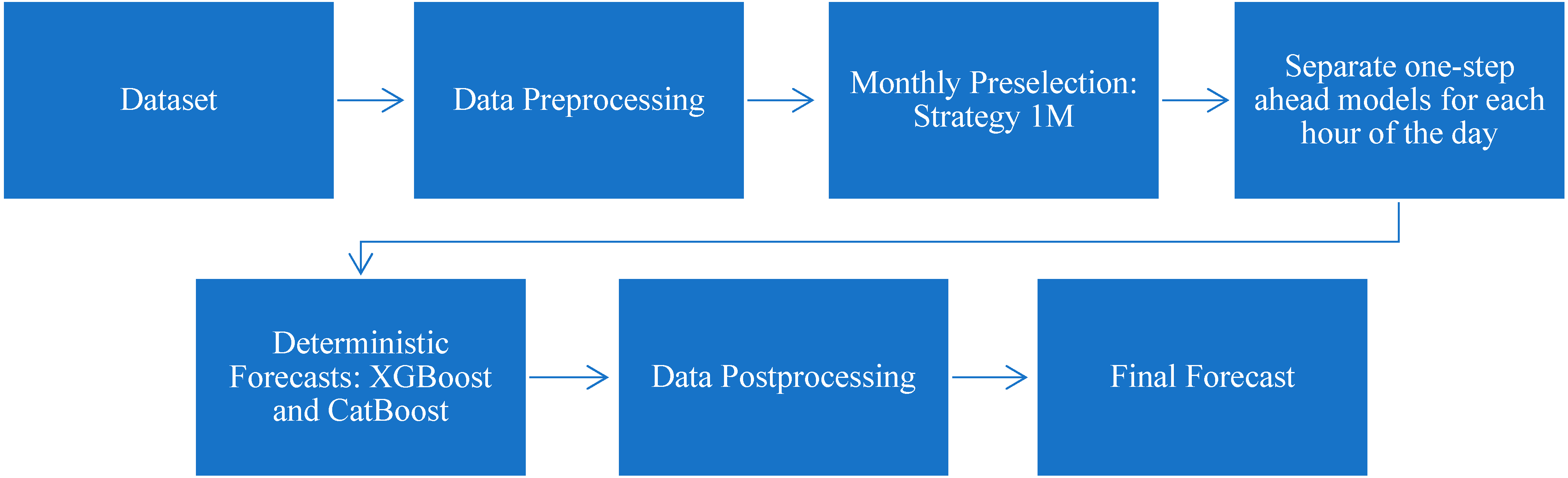
3. Proposed Solar Power Forecasting Methodology

The proposed method comprises relevant inputs, data preprocessing steps, and training of three groups of separate one-step ahead model for each hour of the day, including two regression models per hour to produce a set of deterministic forecasts. The final step considers data postprocessing. These components together form the proposed solar power forecasting framework, presented in Figure 1, which will be described in the following sections.

3.1. Dataset

A dataset with an hourly resolution of PV power output, including lagged power production from the previous 15, 30, 45, 60, and 75 min, and lagged power production from the previous 1, 24, 48, 72, 96, 120, and 144 h from 11 March 2019 to 31 July 2022 are used in this work. Moreover, the following is aggregated in this dataset: Global horizontal irradiance (GHI), zenith, and azimuth. GHI is the total power of solar radiation per unit area, measured in W/m² at a horizontal surface to the ground during the absence of visible clouds across the sky. It provides the maximum irradiance under clear sky conditions. In addition, numerical weather predictions (NWP) are included in the dataset, such as ambient temperature, solar irradiance, wind speed, wind direction, relative humidity, cloud cover, dew point, gust speed, and pressure, in which forecasts are performed by an external source. The solar irradiance forecast considers the likelihood of clouds and their effects on the availability of solar irradiance. In a nearby geographical location of the target PV system, in the City of Medicine Hat, Alberta, Canada, there are more than 20 utility-scale solar farms. Therefore, the historical regional aggregated solar power output (RASPO), and the publicly available regional aggregated solar power predictions (RASPP), which are provided by the independent system operator (ISO) are also added to the dataset. Lagged features or past power production improve the forecast quality since time dependency is considered in the forecasting problem [28]. Data from NWP in solar power forecasting are most applicable for day-ahead forecasting [29]. NWP uses mathematical models of the atmosphere and oceans based on measured conditions to predict with excellent forecast skill up to 6 days ahead and a relatively accurate forecast up to 14 days ahead.

3.2. Data Preprocessing

The standard scaler normalizes all features to remove the mean and scale to unit variance. A correlation analysis is a statistical summary that assists in identifying the strength and direction of the relationship between two variables. Spearman’s correlation is applicable for nonlinear relationships and non-Gaussian distribution, which assumes that the relationship between variables is monotonic and tends to move in the same relative direction but not at a constant rate. An autocorrelation analysis was performed to explore the relevance of lagged features. In addition, a correlation among other variables was carried out. Therefore, only the most relevant and correlated features are used in this study.

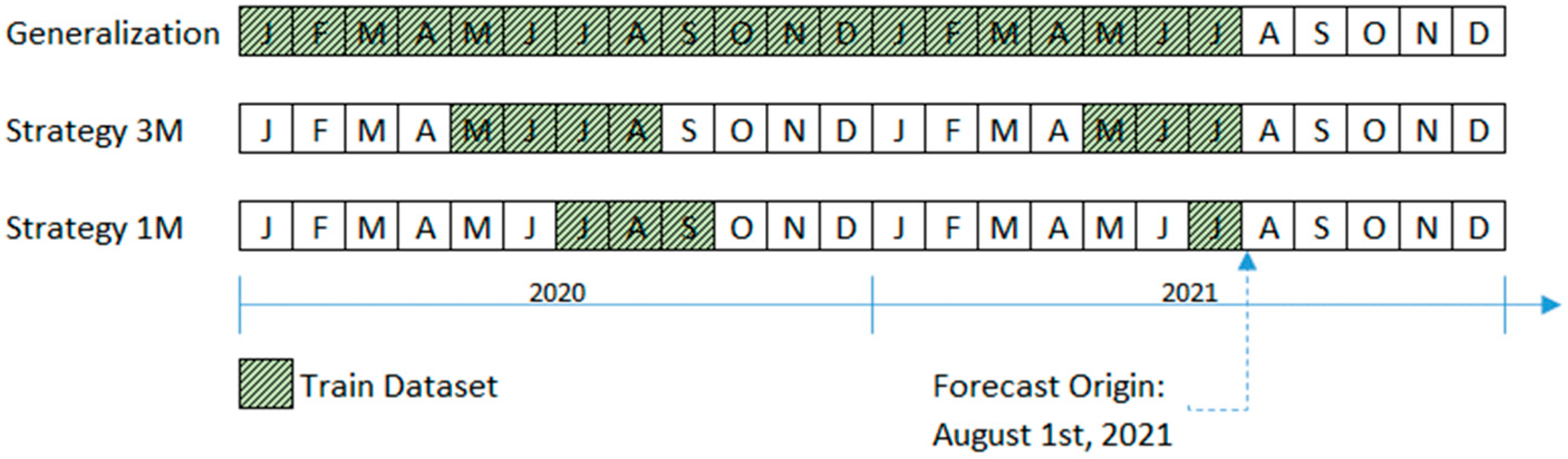
3.3. Monthly Preselection

We propose a new training strategy for this work. The strategy is based on the similarity of seasonal weather and the general solar power production for each month in hourly resolution. For example, the objective is to avoid training with a database from Winter months, while the target is to predict Summer. Two main benefits can be observed: First, the correlation among features is increased, which directly impacts the accuracy of the predictions. Second, the training process speed is increased, which reduces the computational cost.

Herein, primary and secondary strategies are proposed in a simplified way to train a model weekly. Strategy 1M targets the dataset selection of the previous month, the current month, 1 month ahead from the previous year, and the previous month and the last weeks of the current month of the current year, always referenced by the forecasting origin. On the other hand, strategy 3M targets the dataset selection of the previous 3 months of the previous and current year, and the last weeks of the current month of the current year. For example, Figure 2 presents a dataset containing data from 1 January 2020 to 31 December 2021, and the forecast origin is 1 August 2021. For strategy 1M, the preselected months to train the model are from July to September 2020 as well as July 2021. For strategy 3M and the same forecast origin, the preselected months to train the model are from May to August 2020, as well as May to July 2021. Namely, the proposed training strategy 1M considers the typical previous 30 days in the current and previous years, as well as the following 60 days in the previous year. The numerical results in Section 4 highlight the fact that the proposed method can improve the model’s accuracy.

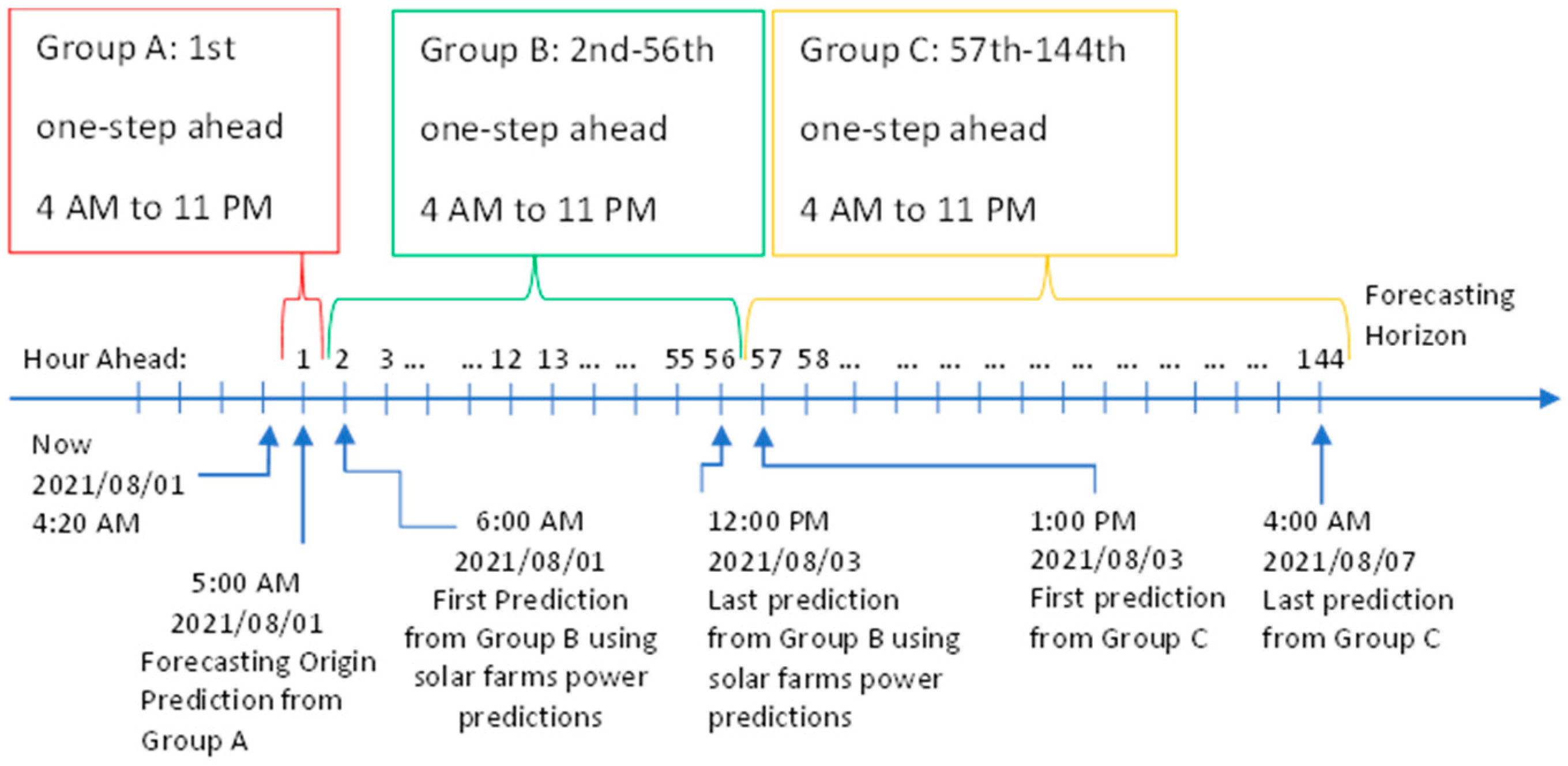
3.4. Separate One-Step Ahead Models for Each Hour of the Day

In this paper, we propose the development of three groups of separate one-step ahead deterministic models, with each group trained for each hour of the day and receiving different inputs. During the Summer, from 4:00 a.m. to 11:00 p.m., there are a total of 20 h of above zero solar irradiance. The strategy does not consider the remaining 4 h of the day since they have zero solar irradiance. Therefore, the proposed methodology trains 20 separate models. In addition, two techniques are selected to fit the models: XGBoost and CatBoost. As a result, the number of separate models per hour multiplied by the number of methods accumulates 40 models per group, and finally, multiplied by three groups results in a total of 120 models. Different combinations of inputs and time horizons are proposed in this work to extract the best outcomes from each available feature and reflect the accuracy gained for each step ahead in the forecasting horizon.

3.4.1. Group A: One-Step Ahead for the 1st Hour Ahead Framework

The most impactful prediction horizon is 1 h ahead since it is critical for monitoring and dispatching purposes. For example, in [30], the authors identified that lagged observations are more important for shorter forecasting horizons than weather forecasts. Group A is a set of one-step models for the 1st hour ahead, with separate models for each hour of the day. It leverages the most recent observations of the target PV system’s power (p) from the previous 15, 30, 45, 60, and 75 min to increase the accuracy of the next hour ahead prediction. In addition, exogenous inputs from NWP, such as GHI, ambient temperature (T), and solar irradiance (SI) are considered, according to Equation (1). For a set of models, M^A with h hours of the day is limited to 4:00 a.m. ≤ h ≤ 11:00 p.m. and two techniques (XGBoost, CatBoost), herein Equation (2) represents Group A, as follows:

$$\left(p_{t+1}\right)=f\left(p_{t-15},p_{t-30},p_{t-45},p_{t-60},p_{t-75},GH{I}_{t+1},T_{t+1},S{I}_{t+1}\right)$$

(1)

$$M^A={\left\{\left(XG{B}_4^A,CT{B}_4^A\right),\dots \left(XG{B}_h^A,CT{B}_h^A\right)\right\}}_{h=4AM,\dots 11PM}$$

(2)

3.4.2. Group B: One-Step Ahead for 2nd to 56th Hour Ahead Framework

Intra-day and day-ahead forecasts are relevant for scheduling the spinning reserve capacity. Group B is a set of one-step ahead models for recursive predictions from the 2nd to the 56th hour ahead, with separate models for each hour of the day. Group B leverages the information from NWP and the solar farms’ power predictions to increase the accuracy of the target PV power output model. Since these forecasts are available with a forecasting horizon limited to the 56th hour ahead, Group B is also determined by the same horizon. The set of inputs considered in this group of models are past power output (p), GHI, ambient temperature (T), solar irradiance (SI), wind speed (WS), relative humidity (RH), and the publicly available regional aggregated solar power predictions (RASPP), according to Equation (3) with k = (2, …, 56). The forecasting engine uses a recursive forecasting strategy, i.e., to keep the properties of the time series, the outputs from Group A are used as inputs to Group B and then from Group B to Group C [31]. For a set of models, M^B with h hours of the day is limited to 4:00 a.m. ≤ h ≤ 11:00 p.m. and two techniques (XGBoost, CatBoost), herein Equation (4) represents Group B, as follows:

$$\left(p_{t+2h},\dots ,p_{t+k}\right)=f\left(p_{t-1h},p_{t-24h},p_{t-48h},p_{t-72h},p_{t-96h},p_{t-120h},p_{t-144h},GH{I}_{t+k},T_{t+k},S{I}_{t+k},W{S}_{t+k},R{H}_{t+k},RASP{P}_{t+k}\right)$$

(3)

$$M^B={\left\{\left(XG{B}_4^B,CT{B}_4^B\right),\dots \left(XG{B}_h^B,CT{B}_h^B\right)\right\}}_{h=4AM,\dots 11PM}$$

(4)

3.4.3. Group C: One-Step Ahead for 57th to 144th Hour Ahead Framework

The following days ahead forecasting is essential for managing the grid operations. Group C is a set of one-step ahead models for recursive predictions from 57th to 144th hour ahead, with separate models for each hour of the day. Group C models rely on the NWP and the most recent forecasts from Group B, following the same recursive forecasting strategy. The input variables are past power output (p), GHI, ambient temperature (T), solar irradiance (SI), wind speed (WS), and relative humidity (RH), according to Equation (5) with k = (57, …, 144). For a set of models, M^C with h hours of the day limited to 4:00 a.m. ≤ h ≤ 11:00 p.m. and two techniques (XGBoost, CatBoost), herein Equation (6) represents Group C, as follows:

$$\left(p_{t+57h},\dots ,p_{t+k}\right)=f\left(p_{t-1h},p_{t-24h},p_{t-48h},p_{t-72h},p_{t-96h},p_{t-120h},p_{t-144h},GH{I}_{t+k},T_{t+k},S{I}_{t+k},W{S}_{t+k},R{H}_{t+k}\right)$$

(5)

$$M^C={\left\{\left(XG{B}_4^C,CT{B}_4^C\right),\dots \left(XG{B}_h^C,CT{B}_h^C\right)\right\}}_{h=4AM,\dots 11PM}$$

(6)

Figure 3 shows an example of the forecasting strategy and how Groups A, B, and C accumulate outputs for the forecasting horizon of 144 h ahead. The instance considers the issuing time of 1 August 2021 at 4:20 a.m.. Therefore, the forecasting origin is 1 August 2021 at 5:00 a.m., which is one step ahead of forecasting. From a set of 20 pairs of models, Group A will select the appropriate model specific for 5:00 a.m. to forecast the first step. It will provide predictions for XGBoost and CatBoost. Next, Group B will predict the second step by selecting the 6:00 a.m. models for the specific hour. Then, Group B sets the next pair of models recursively for 7:00 a.m. until it reaches 56 h ahead of forecast. Similarly, Group C will provide the following one-step forecasting from 57 to 144 h ahead, when the last prediction of the forecasting horizon is reached. In summary, a serial sequence of one-step ahead or 1 h ahead models will be selected from 1 to 144 h ahead.

3.5. Deterministic Forecast

Point forecasts, deterministic forecasts, or single-value forecasts are all synonyms. They can be used to define that the predictions or forecasts made by this class of models can output only one value for each instance or each time stamp. Two deterministic models will be presented and then, individual performances will be evaluated. Producing probabilistic forecasts are left for future works.

• XGBoost (XGB) [32], or the eXtreme Gradient Boosting, is an evolution implementation of the gradient tree boosting (GB), which is a technique first introduced in 2000 by the authors of [33]. XGBoost gained recognition in several data mining challenges and machine learning competitions. For example, in 2017, one of the five best teams in The Global Energy Forecasting Competition 2017 (GEFCom2017) used XGBoost to solve a hierarchical probabilistic load forecasting problem. The technique is a gradient boosted tree algorithm, a supervised learning method capable of fitting generic nonparametric predictive models. For XGBoost, a search for the hyperparameters with RandomizedSearchCV class and GridSearchCV class from Scikitlearn is performed.
• CatBoost (CTB), or categorical boosting [34], is an open-source machine learning tool developed in Germany in 2017. The authors claim that this updated method outperforms the existing state-of-the-art implementations of gradient-boosted decision trees XGBoost. CatBoost proposes ordered boosting, a modification of the standard gradient boosting algorithm that avoids both a target leakage and prediction shift, with a new algorithm for processing categorical features. It presents three main advantages: First, it can integrate data types, such as numerical, images, audio, and text features. Second, it can simplify the feature engineering process since it requires minimal categorical feature transformation. Finally, it has a built-in hyperparameter optimization, which simplifies the learning process while increasing the overall speed of the model.

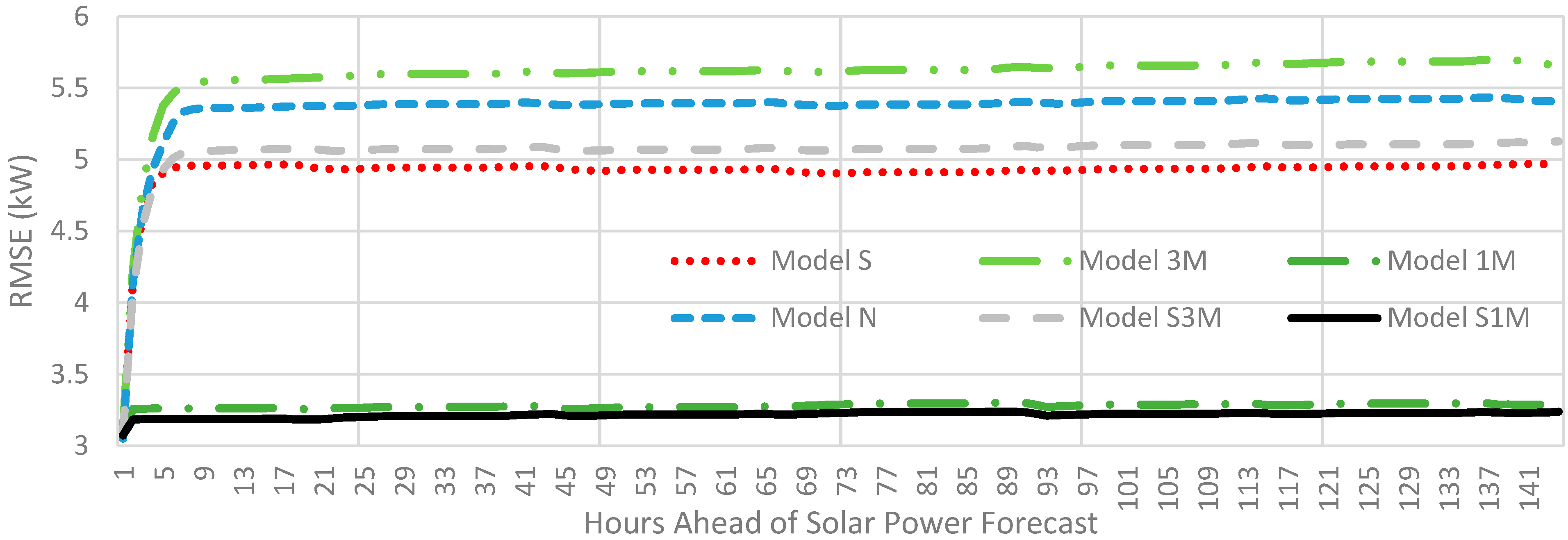
4. Numerical Results

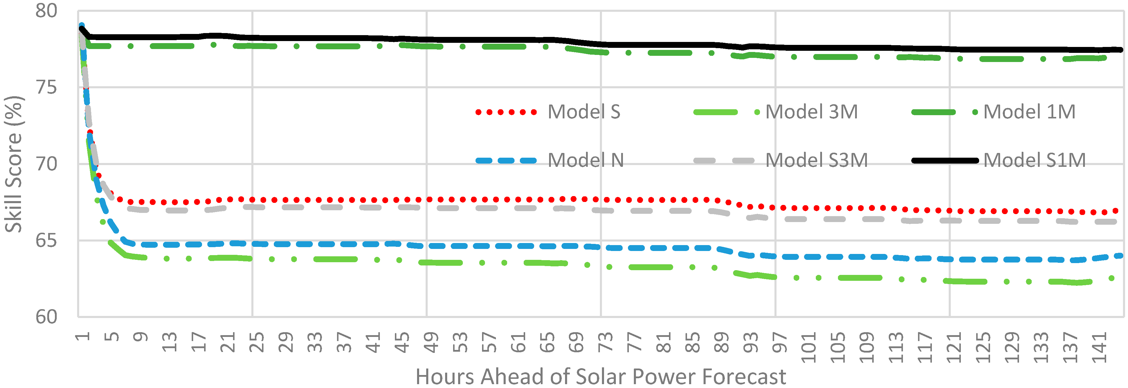
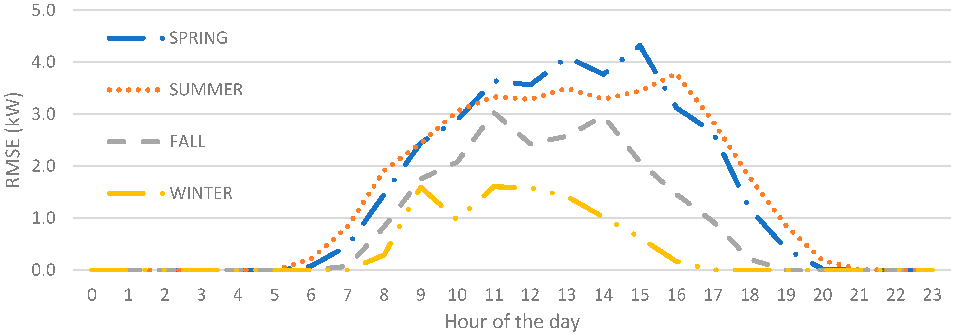
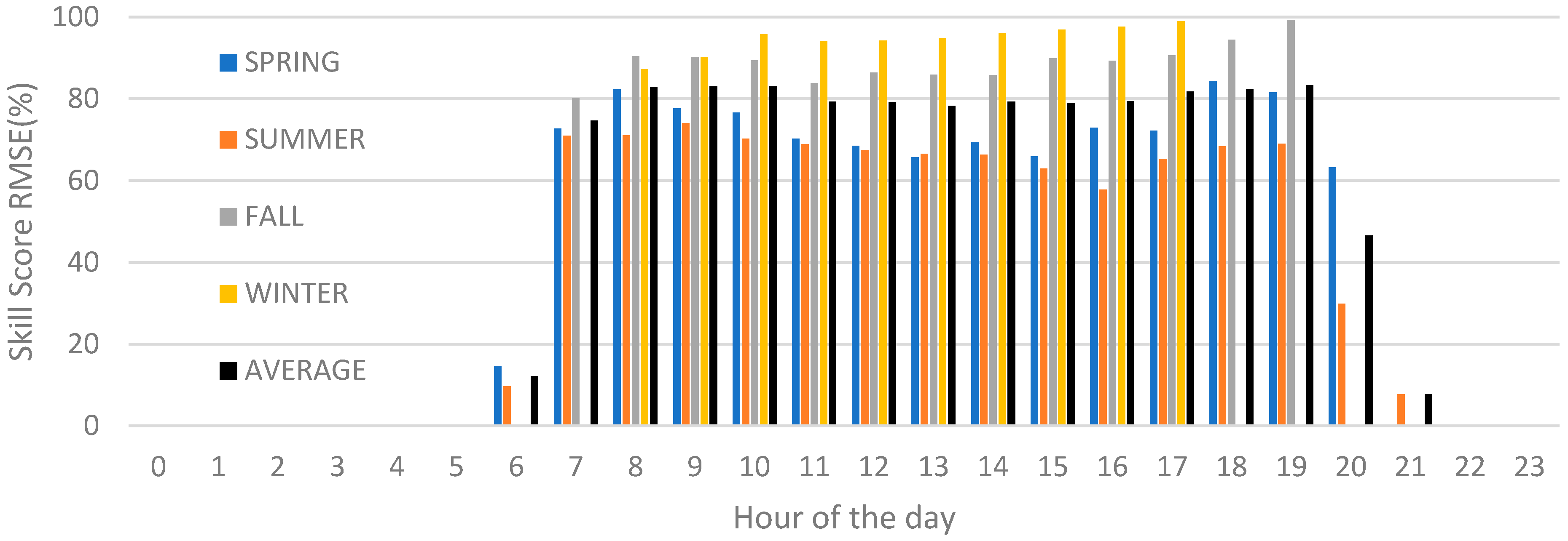
4.1. Evaluation Criteria

The most common and accepted deterministic forecasting accuracy measures are the root mean squared error (RMSE) and its respective RMSE skill score [35,36]. The RMSE is a common error metric used in point forecasting due to its squared error, which is more sensitive to outliers [37]. The RMSE is calculated according to Equation (7). It is measured with the same unit as the target forecasting, in kilowatts (kW). For n = 144, t $\in \left(1,2,\dots 144\right)$, ${\widehat{y}}_t$ is the forecast at time t, and $y_t$ is the observed PV power at time t. The best way to measure the accuracy gain of a proposed forecasting method is to calculate the forecast skill score using the RMSE as the base metric and compare the results from the proposed method versus a benchmark method [35,38]. The RMSE skill score is calculated using Equation (8) and is measured in percent (%), as follows:

$$RMSE=\sqrt{\frac{1}{n}{\displaystyle \sum }_{t=1}^n{\left({\widehat{y}}_t-y_t\right)}^2}$$

(7)

$$SkillScor{e}_{RMSE}=1-\frac{RMS{E}_{ProposedMethod}}{RMS{E}_{Benchmark}}$$

(8)

4.2. Benchmark

Solar energy forecasts, including irradiance and power, strongly depend on data, location, resolution, and horizon. Therefore, according to the author in [35], without a universal benchmark, it is sometimes impossible to interpret the quality of a solar energy forecast model. The complete-history persistence ensemble (CH-PeEn) was proposed in 2019 to be a universal benchmarking method for probabilistic solar forecasting [16]. The historical PV power output with hourly resolution used to calculate this model is from 11 March 2019 to 31 July 2022. This paper will use the percentile 50% or the mean as a benchmark. Figure 4 shows the target PV system’s mean and probability distribution of power.

4.3. Test Design

In this paper, the following six scenarios will be performed to demonstrate the quality of each strategy: Models S, 3M, 1M, N, S3M, and S1M, covering from 1 h to 6 days ahead. First, Model S will verify whether the hybrid method with publicly available regional aggregated solar power predictions can be effectively applied to increase the accuracy of the small-scale BTM PV model. Second, Model 3M will verify whether solely selecting the current and the previous 3 months related to a targeted pattern of historical data can increase the forecasting model accuracy. Third, Model 1M will examine the accuracy improvement from the solely 1M strategy. Fourth, Model N will verify whether a model considering none of the proposed strategies is better and can increase the forecasting model accuracy. Fifth, Model S3M will explore whether a model assuming a combination of Models S and 3M can improve the model’s accuracy. Sixth, Model S1M, the proposed model of this paper, will consider including Models S and 1M. A CH-PeEn model benchmark is also performed to compare the forecasting skill of each model. The training data available are from 11 March 2019 to 31 July 2021. Each model is retrained every week, adding one previous week. The solar power forecasting methodology is deployed to predict a total of 1 year of testing from 1 August 2021 to 31 July 2022.

The skill score RMSE of each model per month and season is presented in

Table 1. Average skill score RMSE (%) per month per model.

INDEX	202108	202109	202110	202111	202112	202201	202202	202203	202204	202205	202206	202207
S-XGBoost	58	69	80	85	91	88	78	67	51	39	52	42
S-CatBoost	59	69	81	86	91	88	79	68	52	41	52	44
3M-XGBoost	52	60	75	82	90	84	77	57	42	47	45	34
3M-CatBoost	53	63	75	84	92	85	78	59	45	46	47	35
1M-XGBoost	72	72	84	91	95	94	89	74	70	55	60	54
1M-CatBoost	72	74	85	91	96	94	90	77	70	57	61	57
N-XGBoost	53	53	73	84	92	85	81	61	48	45	48	35
N-CatBoost	55	56	75	84	92	86	81	62	49	46	51	38
S3M-XGBoost	58	66	77	84	92	84	80	63	48	44	49	43
S3M-CatBoost	58	68	79	85	93	85	80	65	49	45	50	47
S1M-XGBoost	74	74	85	91	95	94	89	76	72	56	61	57
S1M-CatBoost	73	75	85	91	95	94	90	77	70	58	62	58

and

Table 2. Average skill score RMSE (%) per season per model.

INDEX	SPRING	SUMMER	FALL	WINTER	AVG Year	Ranking
S-XGBoost	52	51	78	86	66.7	7
S-CatBoost	54	52	79	86	67.5	5
3M-XGBoost	48	44	72	84	62.2	12
3M-CatBoost	50	45	74	85	63.6	10
1M-XGBoost	67	62	82	93	76.0	4
1M-CatBoost	68	63	83	93	76.8	3
N-XGBoost	52	45	70	86	63.2	11
N-CatBoost	52	48	72	86	64.7	9
S3M-XGBoost	52	50	76	85	65.6	8
S3M-CatBoost	53	52	77	86	67.0	6
S1M-XGBoost	68	64	83	93	76.9	2
S1M-CatBoost	68	64	84	93	77.3	1

, respectively, for models XGBoost and CatBoost. Table 1 shows that from October to February, the skill score ranges from 73% to 96% compared with the CH-PeEn benchmark, in which the skill score is more significant than in the other months. This result aligns with the baseline in Section 4.2 since it has only one shape for all days of the year, represented by the mean curve in Figure 4. For example, in Table 1, the results for S1M-CatBoost show that the highest skill score occurred in December 2021 and the lowest in May and July 2022. This indicates that compared with the benchmark in Figure 4, the general shape and magnitude of the solar power predictions are more similar to months, such as May and July than December. According to the authors of [35], due to an effective model considering a station in the upwind direction to the target point, higher forecast skill scores can be found between 50% and 70% during specific periods and not year round.

In Table 2, it can be observed that strategies S, 3M, N, and S3M presented skill score RMSE results below 67.5%. Moreover, this table shows how Models S1M and 1M are more relevant than the other suggested models. When Model N is compared with Model S1M, it can be observed that Model S1M could leverage the combination of both strategies: S and 1M, indicating that the solar farms’ power forecasts and the reduced dataset assisted in increasing the forecasting skill. The best individual technique was S1M-CatBoost, with an average per year of 77.3%, followed by S1M-XGBoost with 76.9%.

In Table 2, the best deterministic model is CatBoost, since it outperformed XGBoost on all scenarios. Therefore, an analysis of the average RMSE and the skill score RMSE of hours ahead predictions of the six solar scenarios will be presented only for the CatBoost scenarios. Figure 5 shows that Model 3M presents the highest RMSE, while Model 1M is the second best, which indicates that a reduced dataset using strategy 1M leveraged the highest correlation to improve the model’s accuracy. Next, Model N was easily outperformed by Models S3M and S when the publicly available regional aggregated solar power predictions were added as a feature. Finally, the proposed Model S1M consistently outperformed from 2 to 144 h ahead. For Model S1M, the error increases more noticeably from 1 to 2 h ahead, and the average error of the following steps increases very slightly. Moreover, an improvement is observed between steps 91 and 97. It could be related to the recursive forecasting strategy and the lagged power production as inputs for the model, highlighting a higher correlation.

Figure 6 shows that all CatBoost scenarios outperformed the mean of the benchmark CH-PeEn with skill score RMSE ranging from 79% to 62%. Although Models S1M, 1M, S, and S3M were outperformed by Model N via a small margin in the 1st hour ahead, all models outperformed Model N consistently for all of the remaining 143 steps ahead. Models 1M and 3M outperformed the benchmark, but the latter did not outperform Model N any step forward. Finally, Models 1M and 3M were improved when the solar farms’ power predictions were added as a feature, later identified as Models S1M and S3M, proving the relevance of this feature.

Since the best deterministic model is the S1M-CatBoost, an analysis of the average RMSE and skill score RMSE for each hour of the day will be presented. The average RMSE and the respective skill score RMSE for each hour of the day in the four seasons are shown as two main characteristics in Figure 7 and Figure 8. First, each season has a particular magnitude, and second, each has a specific duration, from sunrise to sunset. For example, during Summer, the highest magnitude of RMSE is around 3.8 kW at 4:00 p.m., and the daylight hours are from 6:00 a.m. to 9:00 p.m., with an average skill score of 65%. However, during Winter, the lowest magnitude of RMSE is found since it is directly proportional to the lower availability of solar irradiance, around 1.6 kW at 9:00 a.m., with daylight hours from 8:00 a.m. to 5:00 p.m., and an average skill score of 93%.

In Figure 8, the average skill score identified from 7:00 a.m. to 7:00 p.m. for all seasons are similar, but two exceptions can be found. During Spring and Summer, at 6:00 a.m. and 8:00 p.m., and during Summer, at 9:00 p.m., the magnitude of the skill score is lower than the season average. This situation occurs due to the higher errors found, especially during sunrise and sunset, which are harder to predict even though the magnitude of the PV output is significantly lower than the daylight peak hours.

5. Conclusions

The contributions of this paper are three-fold: First, a new hybrid methodology was proposed with a sequence of one-step models to forecast 6 days ahead for a small-scale BTM PV site with three groups of models with different inputs—each group was trained for each hour of above zero irradiance. The best technique identified was CatBoost and the proposed method was S1M. Second, a novel dataset preselection was presented, named 1M, and individual results proved the method’s efficiency against a benchmark and other scenarios. Third, applying neighboring solar farm predictions as a feature boosted the model’s accuracy. Therefore, to the author’s knowledge, no other research work has developed a simplified targeted training strategy, such as the one presented or used publicly available regional aggregated solar power predictions from neighboring utility-scale solar farms to improve the quality of the small-scale BTM PV system forecasts.

Future Work

Probabilistic forecasts describe the embedded variability and assist in the decision-making process [18]. Therefore, a bootstrap strategy can be implemented by creating N different scenarios with an increased bandwidth of predictions to output a probabilistic forecast. For example, the authors of [24] used 20,000 weather scenarios and averaged the estimates with quantile regression averaging (QRA) to produce probabilistic forecasts.

References

1. Masson, G. International Energy Agency Snapshot. 2022. Available online: https://iea-pvps.org/snapshot-reports/snapshot-2022/ (accessed on 11 August 2022).
2. Haupt, S.E.; Dettling, S.; Williams, J.K.; Pearson, J.; Jensen, T.; Brummet, T.; Kosovic, B.; Wiener, G.; McCandless, T.; Burghardt, C. Blending Distributed Photovoltaic and Demand Load Forecasts. Sol. Energy 2017, 157, 542–551. [Google Scholar] [CrossRef]
3. Chu, Y.; Pedro, H.T.C.; Kaur, A.; Kleissl, J.; Coimbra, C.F.M. Net Load Forecasts for Solar-Integrated Operational Grid Feeders. Sol. Energy 2017, 158, 236–246. [Google Scholar] [CrossRef]
4. Kaur, A.; Nonnenmacher, L.; Pedro, H.T.C.; Coimbra, C.F.M. Benefits of Solar Forecasting for Energy Imbalance Markets. Renew. Energy 2016, 86, 819–830. [Google Scholar] [CrossRef]
5. Mellit, A.; Pavan, A.M.; Ogliari, E.; Leva, S.; Lughi, V. Advanced Methods for Photovoltaic Output Power Forecasting: A Review. Appl. Sci. 2020, 10, 487. [Google Scholar] [CrossRef]
6. Dolara, A.; Grimaccia, F.; Leva, S.; Mussetta, M.; Ogliari, E. A Physical Hybrid Artificial Neural Network for Short Term Forecasting of PV Plant Power Output. Energies 2015, 8, 1138–1153. [Google Scholar] [CrossRef]
7. Cervone, G.; Clemente-Harding, L.; Alessandrini, S.; Delle Monache, L. Short-Term Photovoltaic Power Forecasting Using Artificial Neural Networks and an Analog Ensemble. Renew. Energy 2017, 108, 274–286. [Google Scholar] [CrossRef]
8. Yagli, G.M.; Yang, D.; Srinivasan, D. Automatic Hourly Solar Forecasting Using Machine Learning Models. Renew. Sustain. Energy Rev. 2019, 105, 487–498. [Google Scholar] [CrossRef]
9. Zhang, X.; Li, Y.; Lu, S.; Hamann, H.F.; Hodge, B.M.; Lehman, B. A Solar Time Based Analog Ensemble Method for Regional Solar Power Forecasting. IEEE Trans. Sustain. Energy 2019, 10, 268–279. [Google Scholar] [CrossRef]
10. Wolff, B.; Kühnert, J.; Lorenz, E.; Kramer, O.; Heinemann, D. Comparing Support Vector Regression for PV Power Forecasting to a Physical Modeling Approach Using Measurement, Numerical Weather Prediction, and Cloud Motion Data. Sol. Energy 2016, 135, 197–208. [Google Scholar] [CrossRef]
11. Mellit, A.; Massi Pavan, A.; Lughi, V. Short-Term Forecasting of Power Production in a Large-Scale Photovoltaic Plant. Sol. Energy 2014, 105, 401–413. [Google Scholar] [CrossRef]
12. Yang, C.; Xie, L. A Novel ARX-Based Multi-Scale Spatio-Temporal Solar Power Forecast Model. In Proceedings of the 2012 North American Power Symposium, NAPS 2012, Champaign, IL, USA, 9–11 September 2012. [Google Scholar] [CrossRef]
13. Goncalves, C.; Bessa, R.J.; Pinson, P. Privacy-Preserving Distributed Learning for Renewable Energy Forecasting. IEEE Trans. Sustain. Energy 2021, 12, 1777–1787. [Google Scholar] [CrossRef]
14. Antonanzas, J.; Osorio, N.; Escobar, R.; Urraca, R.; Martinez-de-Pison, F.J.; Antonanzas-Torres, F. Review of Photovoltaic Power Forecasting. Sol. Energy 2016, 136, 78–111. [Google Scholar] [CrossRef]
15. Yang, D. Standard of Reference in Operational Day-Ahead Deterministic Solar Forecasting. J. Renew. Sustain. Energy 2019, 11, 053702. [Google Scholar] [CrossRef]
16. Yang, D. A Universal Benchmarking Method for Probabilistic Solar Irradiance Forecasting. Sol. Energy 2019, 184, 410–416. [Google Scholar] [CrossRef]
17. Pedro, H.T.C.; Coimbra, C.F.M.; David, M.; Lauret, P. Assessment of Machine Learning Techniques for Deterministic and Probabilistic Intra-Hour Solar Forecasts. Renew. Energy 2018, 123, 191–203. [Google Scholar] [CrossRef]
18. van der Meer, D. Comment on “Verification of Deterministic Solar Forecasts”: Verification of Probabilistic Solar Forecasts. Sol. Energy 2020, 210, 41–43. [Google Scholar] [CrossRef]
19. Pedro, H.T.C.; Coimbra, C.F.M. Assessment of Forecasting Techniques for Solar Power Production with No Exogenous Inputs. Sol. Energy 2012, 86, 2017–2028. [Google Scholar] [CrossRef]
20. Panamtash, H.; Zhou, Q.; Hong, T.; Qu, Z.; Davis, K.O. A Copula-Based Bayesian Method for Probabilistic Solar Power Forecasting. Sol. Energy 2020, 196, 336–345. [Google Scholar] [CrossRef]
21. Marquez, R.; Pedro, H.T.C.; Coimbra, C.F.M. Hybrid Solar Forecasting Method Uses Satellite Imaging and Ground Telemetry as Inputs to ANNs. Sol. Energy 2013, 92, 176–188. [Google Scholar] [CrossRef]
22. Huang, J.; Perry, M. A Semi-Empirical Approach Using Gradient Boosting and k-Nearest Neighbors Regression for GEFCom2014 Probabilistic Solar Power Forecasting. Int. J. Forecast. 2016, 32, 1081–1086. [Google Scholar] [CrossRef]
23. Pierro, M.; Gentili, D.; Liolli, F.R.; Cornaro, C.; Moser, D.; Betti, A.; Moschella, M.; Collino, E.; Ronzio, D.; van der Meer, D. Progress in Regional PV Power Forecasting: A Sensitivity Analysis on the Italian Case Study. Renew. Energy 2022, 189, 983–996. [Google Scholar] [CrossRef]
24. Sun, M.; Feng, C.; Zhang, J. Probabilistic Solar Power Forecasting Based on Weather Scenario Generation. Appl. Energy 2020, 266. [Google Scholar] [CrossRef]
25. Pinho, M.; Muñoz, M.; De, I.; Perpiñán, O. Comparative Study of PV Power Forecast Using Parametric and Nonparametric PV Models. Sol. Energy 2017, 155, 854–866. [Google Scholar] [CrossRef]
26. Lonij, V.P.A.; Brooks, A.E.; Cronin, A.D.; Leuthold, M.; Koch, K. Intra-Hour Forecasts of Solar Power Production Using Measurements from a Network of Irradiance Sensors. Sol. Energy 2013, 97, 58–66. [Google Scholar] [CrossRef]
27. Vaz, A.G.R.; Elsinga, B.; van Sark, W.G.J.H.M.; Brito, M.C. An Artificial Neural Network to Assess the Impact of Neighbouring Photovoltaic Systems in Power Forecasting in Utrecht, the Netherlands. Renew. Energy 2016, 85, 631–641. [Google Scholar] [CrossRef]
28. Henze, J.; Schreiber, J.; Sick, B. Representation Learning in Power Time Series Forecasting; Springer International Publishing: Kassel, Germany, 2020; ISBN 9783030317607. [Google Scholar]
29. Zhang, G.; Yang, D.; Galanis, G.; Androulakis, E. Solar Forecasting with Hourly Updated Numerical Weather Prediction. Renew. Sustain. Energy Rev. 2022, 154, 111768. [Google Scholar] [CrossRef]
30. Persson, C.; Bacher, P.; Shiga, T.; Madsen, H. Multi-Site Solar Power Forecasting Using Gradient Boosted Regression Trees. Sol. Energy 2017, 150, 423–436. [Google Scholar] [CrossRef]
31. ben Taieb, S.; Hyndman, R.J. Recursive and Direct Multi-Step Forecasting: The Best of Both Worlds. Int. J. Forecast. Available online: https://www.monash.edu/business/ebs/research/publications/ebs/wp19-12.pdf (accessed on 11 August 2022).
32. Chen, T.; Guestrin, C. XGBoost: A Scalable Tree Boosting System. In Proceedings of the 22nd ACM SIGKDD International Conference on Knowledge Discovery and Data Mining, San Francisco, CA, USA, 13–17 August 2016; ACM: New York, NY, USA, 2016; Volume 42, pp. 785–794. [Google Scholar]
33. Friedman, J.; Tibshirani, R.; Hastie, T. Additive Logistic Regression: A Statistical View of Boosting (With Discussion and a Rejoinder by the Authors). Ann. Stat. 2000, 28, 337–407. [Google Scholar] [CrossRef]
34. Prokhorenkova, L.; Gusev, G.; Vorobev, A.; Dorogush, A.V.; Gulin, A. Catboost: Unbiased Boosting with Categorical Features. Adv. Neural Inf. Process. Syst. 2018, 6638–6648. [Google Scholar]
35. Yang, D. A Guideline to Solar Forecasting Research Practice: Reproducible, Operational, Probabilistic or Physically-Based, Ensemble, and Skill (ROPES). J. Renew. Sustain. Energy 2019, 11. [Google Scholar] [CrossRef]
36. Pedro, H.T.C.; Larson, D.P.; Coimbra, C.F.M. A Comprehensive Dataset for the Accelerated Development and Benchmarking of Solar Forecasting Methods. J. Renew. Sustain. Energy 2019, 11. [Google Scholar] [CrossRef]
37. van der Meer, D.W.; Widén, J.; Munkhammar, J. Review on Probabilistic Forecasting of Photovoltaic Power Production and Electricity Consumption. Renew. Sustain. Energy Rev. 2018, 81, 1484–1512. [Google Scholar] [CrossRef]
38. Nonnenmacher, L.; Kaur, A.; Coimbra, C.F.M. Day-Ahead Resource Forecasting for Concentrated Solar Power Integration. Renew Energy 2016, 86, 866–876. [Google Scholar] [CrossRef]
Figure 1. The proposed solar power forecasting methodology.
Energies 16 01533 g001
Figure 2. The proposed training strategy.
Energies 16 01533 g002
Figure 3. Group A, B, and C models to predict 1-144 h ahead.
Energies 16 01533 g003
Figure 4. The dashed dark blue line represents the mean, and the light blue area represents the 90% interval probability distribution of power for the CH-PeEn benchmark for the target PV system for six consecutive days.
Energies 16 01533 g004
Figure 5. RMSE of hours ahead predictions of the six CatBoost scenarios.
Energies 16 01533 g005
Figure 6. Skill score RMSE of hours ahead predictions of the six CatBoost scenarios.
Energies 16 01533 g006
Figure 7. Average RMSE for each hour of the day for the proposed Model S1M.
Energies 16 01533 g007
Figure 8. Average skill score RMSE for each hour of the day for the proposed Model S1M.
Energies 16 01533 g008