Data-Driven Prediction of Unsteady Vortex Phenomena in a Conical Diffuser

Abstract

The application of machine learning to solve engineering problems is in extremely high demand. This article proposes a tool that employs machine learning algorithms for predicting the frequency response of an unsteady vortex phenomenon, the precessing vortex core (PVC), occurring in a conical diffuser behind a radial swirler. The model input parameters are the two components of the time-averaged velocity profile at the cone diffuser inlet. An empirical database was obtained using a fully automated experiment. The database associates multiple inlet velocity profiles with pressure pulsations measured in the cone diffuser, which are caused by the PVC in the swirling flow. In total, over 10³ different flow regimes were measured by varying the swirl number and the cone angle of the diffuser. Pressure pulsations induced by the PVC were detected using two pressure fluctuations sensors residing on opposite sides of the conical diffuser. A classifier was constructed using the Linear Support Vector Classification (Linear SVC) model and the experimental data. The classifier based on the average velocity profiles at the cone diffuser inlet allows one to predict the emergence of the PVC with high accuracy (99%). By training a regression artificial neural network, the frequency response of the flow was predicted with an error of no more than 1.01 and 5.4% for the frequency and power of pressure pulsations, respectively.

1. Introduction

Hydropower is one of the most environmentally friendly forms of electricity generation, accounting for about 68% of the world’s renewable energy capacity. The use of low-diversity thermal and nuclear power plants, as well as the introduction of unstable technologies such as wind and solar into the grid, suggests that hydropower plays a critical regulating role in maintaining stable grid operation. This is achieved by operating hydro turbines in a wide range of regimes. These regimes are often far from the optimal regimes for which they were originally designed.

In the non-optimal operating regime, the flow behind the runner at the draft tube inlet has excessive swirl, i.e., a high tangential velocity component. In combination with the expanding part of the hydraulic turbine draft tube, this leads to the formation of a precessional vortex core (PVC) in the flow, also known as the rotating vortex rope (RVR). The PVC is a vortex structure that rotates around its own axis and also performs precession motion by deviating from the central axis of symmetry. The PVC generates periodic pressure pulsations in the flow path, which are extremely dangerous due to their potential resonance with the natural frequencies of vibrations of various types that occur in hydroelectric power stations.

Rheingans [1] was among the first scientists to draw attention to the problem of unsteady vortex phenomena in flowing hydraulic turbine systems. He has related hydroelectric power fluctuations to the unsteady phenomena occurring in the flow path, and attempted to classify and describe it. More detailed systematic descriptions were outlined a few decades later in a monograph [2] and in the relatively recent reviews on this topic [3,4]. The main conclusion of the above works is that a powerful precessing vortex rope can lead to fatigue damage and structural failure under a range of operating conditions.

Modern measuring systems have enabled a better understanding of individual flow regimes. Two main types of pressure pulsations in the flow path associated with the presence of PVCs have been identified. These are asynchronous and synchronous pressure pulsations. The asynchronous component is the local pressure pulsations in the draft tube associated with the rotational motion of the vortex core around the central axis. The synchronous component has the same amplitude and phase in the cross section; such pulsations are generated by the interaction between the vortex rope and the draft tube elbow, and propagate throughout the flow path. From an analytical standpoint, the mechanism of occurrence of synchronous pulsations was described in sufficient detail in [5]. A number of features of the swirling flow have been found in the “upper part load” turbine regime. Typically, the precession frequency divided by the runner speed varies between 0.2 and 0.4; however, Nicolet et al. [6] recorded a pulsation frequency one order of magnitude higher than the expected values, which was attributed to a jump-like change in the vortex shape. In the “deep part load” regimes, the PVC exists in the form of a large entanglement of small vortices observed behind the runner [7]. Wahl and Skripkin [8,9] studied vortex splitting into two spiral left-handed vortices rotating in opposite phases, which resulted in unpredictable changes in precession frequency. Vortex splitting is a significant problem in predicting non-stationary flow characteristics. Müller et al. [10] investigated self-excited pressure oscillations in a full-load regime in which an axisymmetric cavity is formed. The pulsations of this cavity lead to the interaction between the fluid column and moving elements of the turbine, thus causing significant power fluctuations. Articles [8,11,12,13] revealed the phenomenon of vortex rope reconnection due to which cavitating vortex rings are formed in the flow. This phenomenon was found to be the source of aperiodic pressure pulsations, previously referred to as the “pressure shock phenomenon” [2].

Despite the intensive research into the vortex flow in various hydraulic turbine operating regimes, it has not yet been possible to establish a clear relationship between the operating parameters and the amplitude-frequency characteristics of the PVC. Nevertheless, [14] managed to show that it is possible to design axial vane swirlers that reproduce predetermined average velocity distributions, or to solve the inverse problem and calculate the average velocity profiles at the draft tube inlet after the impeller according to the impeller geometry. Therefore, all that is left to do is to find the relationship between the characteristics of the PVC and the average velocity distributions at the inlet of the draft tube of the hydraulic turbine.

The first attempts to relate unsteady vortex structures to integral flow characteristics date back to the 1960s. Thus, the integral flow swirl parameter S [15] was introduced as the simplest empirical criterion for the formation of unsteady phenomena in the flow. This dimensionless parameter is defined as the ratio between the flux of momentum torque in the axial direction and the flux of momentum in the axial direction, taking into account the contribution from turbulent stresses and pressure distribution in the flow. In the real world, however, pressure distribution and turbulent fluctuations are neglected when calculating the swirl parameter. The integration of velocity and the large number of assumptions lead to the fact that it becomes impossible to unambiguously relate the unsteady characteristics of the swirling flow to a single numerical parameter. Nevertheless, the critical swirl number (S > 0.6) was introduced in the review [16], from which a PVC and a central recirculation zone are formed in the swirling flow. The introduced value of 0.6 is highly conditional, depends on a large number of boundary conditions, and can only serve as a rough criterion for the emergence of coherent vortex structures, without any information about their frequency characteristics.

More advanced approaches to describing the vortex rope or PVC dynamics can be found in [17,18,19,20]. Kuibin et al. developed a semiempirical model predicting the precession frequency in the draft tube, taking into account the helical shape of the PVC. Alligne et al. developed a one-dimensional draft tube model to predict cavitation pressure pulsations under partial and full load conditions. The model is derived from the flow and continuity equations, including convective terms that were not accounted for in earlier models. Susan-Resiga et al. obtained an analytical representation of the swirl flow, where the dimensionless flow rate was an independent variable. They found that average velocity distributions can be represented as a superposition of three elementary vortices. Pasche and Müller interpreted the vortex rope as a global mode based on linear global stability analysis [21,22,23]. Near the vortex breakdown point, the spiral perturbation develops around the time-averaged flow field, and grows over time to form a precessing vortex. The frequency and structure of this unstable mode agree well with numerical simulations. Nevertheless, the aforementioned models and approaches are imperfect and have significant limitations in their area of applicability. In addition to measuring the mean velocity distributions, parametric models require determining the precession radius, helix pitch, and vortex core size. Calculating these quantities also introduces additional uncertainty due to the lack of generally accepted definitions. Linear analysis requires high-speed PIV measurements with high-precision calibration, but optical access in model hydro turbines is often difficult.

Computer modeling methods describing the turbulent dynamics using numerical solutions of the Navier–Stokes equation are being developed in parallel with experimental modeling, especially with the current rate of computing power growth. Depending on the situation, a wide range of modern turbulence models are used to describe the turbulent flow, e.g., the popular URANS vorticity models (k-ε realizable, k-ω SST), the nonstationary RSM LRR (Launder-Reece and Rodi) Reynolds stress model, the detached vortex model (DDES), the k-ω SST Menter model, and the Large Eddy Simulation (LES) method with the WALE model of subgrid viscosity [24,25]. The main advantage of using numerical simulation is obtaining information about the flow structure in areas inaccessible to optical methods [26]. Another advantage is the freedom to choose the velocity profile distribution as a boundary condition, which is not limited by the technical difficulties related to its implementation on an experimental rig [27]. Numerical modeling methods also allow one to solve the problem of predicting the occurrence of the PVC in a flow including determining the intensity and frequency of pulsations. However, this tool can be used only as an accompanying cross-verification tool to identify the conditions for the formation of precessing vortex structures in a wide range of vortex flows.

The main drawbacks of numerical simulations include the strict requirements for computational power in the nonstationary formulation of the task. Sensitivity of the solution to the selected turbulence model and its parameters is manifested on large grids for the spatial resolution of the minimum possible vortex scales. The complex, multiphase structure of the flow in hydraulic turbines requires permanent verification with the experimental data. All the aforementioned facts indicate that a modern, more accurate mathematical model for describing the characteristics of nonstationary vortex phenomena in hydraulic turbines needs to be developed. The solution to this problem can be found using modern machine learning techniques.

In the literature, there are numerous examples of using machine learning techniques to solve a number of aeronautical problems for modeling empirical patterns, fault diagnosis, and control. Thus, neural networks can be used to implement active control devices to exploit or suppress unsteady aerodynamic phenomena such as dynamic stall on propeller blades. Another challenge is the parallel processing of data obtained from a large number of sensors (from 10 to 1000) for control purposes or for monitoring and fault detection in system components. Neural networks can be effectively used as control algorithms for unstable vehicle maneuvers with six degrees of freedom, when linearized equations of motion do not adequately describe the vehicle dynamics [28]. In the early 1990s, a number of neural network applications were developed to analyze particle trajectory and velocity fields for the Particle Tracking Velocimetry (PTV) and Particle Image Velocimetry (PIV) methods [29,30], and to determine phase configurations in multiphase flows [31]. The connection between low-dimensional dynamic systems modeling techniques (Proper Orthogonal Decomposition) and neural networks [32] has been used to reconstruct turbulent flow fields and flow in the near-wall region of channel flow using information only at the channel wall [33]. Liu and Fang [34] proposed a Bayesian–Gaussian neural network (BGNN) model to design a hydraulic turbine controller. The neural network was used to construct a nonlinear dynamic model of a controlled hydraulic turbine, which was used as an on-line predictive model. Neural networks based on the back propagation algorithm have been successfully applied to predict heat transfer coefficients from a given set of experimentally derived conditions [35]. Pierret and Van den Braembussche described a method for automatically designing turbine blades characterized by improved efficiency [36]. The method has been applied to different types of 2D turbine blades. An artificial neural network was used to construct an approximate model using a database containing solutions to the Navier–Stokes equation for all previous configurations. This approximated model was used to optimize the blade geometry, which was then analyzed by a Navier–Stokes solver. The method allowed one to design more efficient blades while observing both aerodynamic and mechanical limitations, as well as speed up the design process by reducing the time of operator intervention and computational calculations. Abdurakipov et al. [37] studied different machine learning models for the problem of modeling the amplitude-frequency characteristics of the tonal noise that occurs during profile streamlining. Different types of algorithms were analyzed: from the linear to neural network algorithms. The models of regression of pressure amplitude, and classification of modes with high level of tone noise depending on dimensionless flowing parameters were constructed. The implemented model of gradient boosting with the determination coefficient of 95% was shown to be most accurate for describing the spectral curves of acoustic pressure in the entire interval of amplitudes and characteristic frequencies.

The studies [38,39] focused on the swirling flow in cyclone separators. The pressure drop for a cyclone separator is one of the main parameters characterizing its efficiency during the designing stage. A number of neural networks have been developed to accurately predict the complex nonlinear relationships between pressure drop and geometric parameters: the neural network based on the inverse error propagation method and on radial basis functions, as well as the generalized regression neural network.

The applications of neural network techniques to describe flow regimes in hydraulic turbines can be found in [40,41,42]. Hočevar et al. used a network of radial-baseline functions as activation functions to reconstruct the draft tube wall pressure signal from high-speed PVC visualization data in the draft tube cone [42]. This work was further developed in the inverse problem [41], where the pressure signal was used to reconstruct the flow pattern (visualization of the vortex rope in the flow). Ahmed and Raghavan also used an artificial neural network based on radial basis functions to determine the turbulent swirling flow in a model combustion chamber [43]. A more complex problem was considered in [44]; the lifting force and drag were predicted from local velocity measurements while flowing around a cylinder, and the full three-dimensional velocity field was reconstructed. The authors used several deep neural networks that were extended to solve the Navier–Stokes equation for an incompressible fluid together with an equation for the dynamic characteristics of the bluff body.

Neural networks are widely used in fluid mechanics for modeling stochastic dynamical systems. Early examples include the use of neural networks to find solutions to differential equations, but this direction is being intensively developed as evidenced by refs. [44,45], where more complex neural network architectures (discrete and continuous-time neural networks) are applied.

The ML approach to determine inlet boundary conditions for a numerical simulation is proposed in [46,47]. Its goal is to use any known downstream data about the flow to determine the optimal upstream inlet boundary conditions. The proposed approach is applied to the test case of the swirling flow inside a conical diffuser using both RANS k-ω SST and LES turbulence models. The results obtained with the ML approach are found to be in good agreement with the experimental data, and the numerical predictions are improved. We can refer to [48] as a review, one of its conclusions being the successful demonstration that machine learning methods can accurately model complex relationships between the input and output parameters, taking into account the various nonlinear characteristics of fluid flows.

For swirling flows behind a hydraulic turbine runner, there are almost no similar studies involving accumulation of the experimental data and subsequent use of regression analysis methods by building and training neural networks. Nonetheless, the task of predicting the vortex phenomenon at the design stage seems quite adequate taking into account the current advances in machine learning methods.

Therefore, our study aimed to present the potential of machine learning algorithms for predicting the unsteady vortex phenomenon under simplified experimental conditions. For this purpose, we used a swirling air flow behind a radial swirler that expands in a conical diffuser with different conical angles. Vortex breakdown in a form of precessing vortex core occurs under these conditions, resulting in strong coherent pressure pulsations on the walls of the conical diffuser. Flow swirl and the opening angle of the cone diffuser are some of the main parameters that contribute most significantly to the flow structure. Liu et al. [49] showed that different characteristics of the swirling flow in a model hydraulic turbine for three cone angles: 0°, 2°, and 4° are implemented. Thus, by varying these two quantities, we have covered a significant class of vortex flows.

In this paper, an array of empirical data, including the average velocity profiles at the diffuser inlet and pressure fluctuations signals on the walls, was accumulated to train the machine learning algorithm. The paper thoroughly describes the methodology for automated accumulation of empirical data, primary data analysis, training, and testing a machine-learning-based tool for predicting PVC and its power-frequency characteristics.

2. Research Methods

The chapter describes the choice of parameters to study the flow, the experimental setup, the procedure for automating the setup to obtain an array of empirical data, the flow study methods, and the machine learning methods used to build a tool for predicting the PVC in the flow.

2.1. Physical Flow Parameters

Let us set the defining parameters for swirling single-phase and incompressible flows. Such flows are typically characterized by two dimensionless parameters. The first one determines the contribution of the effects of viscosity of the flow medium at the considered flow scale, i.e., the Reynolds number. $Re=\frac{UD}{\nu }$ (where D is the characteristic size; $U$ is the characteristic velocity; ν is the kinematic viscosity). The second one characterizes the relationship between the tangential and axial components of motion, the swirl parameter S:

$$S=\frac{2G_{zz}}{D\cdot G_z},$$

(1)

where, neglecting pressure and turbulent fluctuations of velocity field, the value $G_{zz}=2\pi \rho {{\displaystyle \int }}_0^{\infty }{V}_{ax}{V}_{tg}{r}^{2}dr$ represents the flux of angular momentum in the axial direction of the flow, and the value $G_z=2\pi \rho {{\displaystyle \int }}_0^{\infty }{V}_{ax}^{2}rdr$ represents the momentum flux in the axial direction of the flow; here, r is the radial coordinate V_ax, V_tg are the axial and tangential velocity components, respectively.

When a periodic-time vortex phenomenon in the form of PVC occurs in a swirling flow, its dimensionless frequency is usually represented by the Strouhal number $Sh=f_{PVC}D/U$, where f_PVC is the PVC frequency, i.e., the frequency of the dominant peak in the spectrum of velocity or pressure fluctuations [50]. In swirling flows, the frequency characteristic of the PVC usually depends weakly on the Re number, beginning with Re > 10⁴ [16,51,52]. Meanwhile, the swirl number S remains a parameter determining the structure of the swirling flow [16,53,54,55]. As mentioned above, vortex breakdown occurs at a critical value of S > 0.5–0.6 [16]. As noted in a number of papers [8,56], the criterion does not always uniquely characterize the geometry of the vortex flow, since different vortex structures can be observed at the same swirl numbers, which necessitates using additional geometric parameters, such as the average axial velocity on the vortex chamber axis or pitch of the helical structure [50,56].

In this paper, we study the swirling flow behind a radial swirler, which then enters a conical diffuser with different cone angles. This means that, for the same inlet value of the swirl parameter S, the point of vortex breakdown can move along the axial direction, thus changing the power-frequency characteristics of pressure fluctuations in the cone.

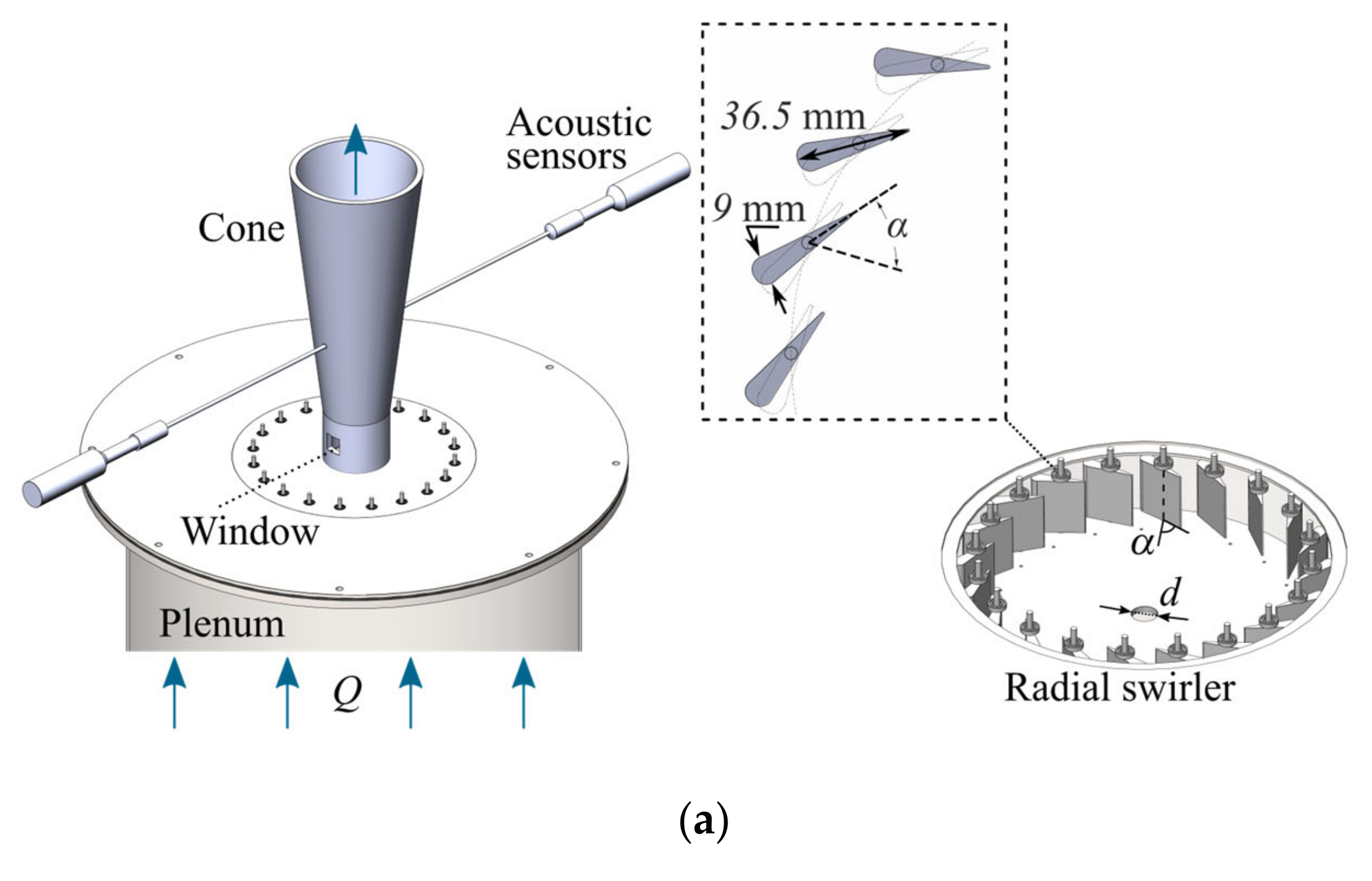
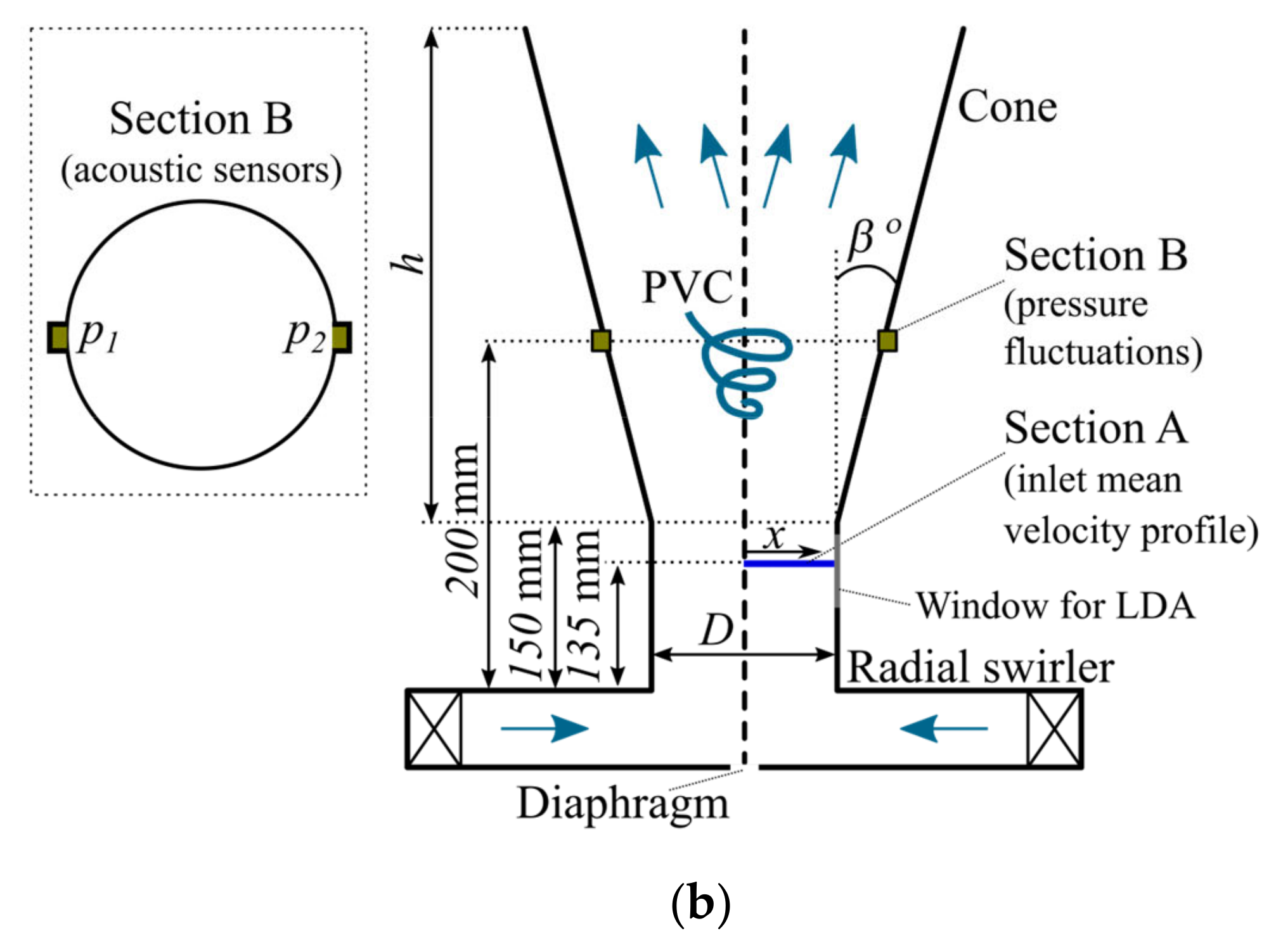
2.2. Experimental Setup

A universal aerodynamic experimental setup was designed and constructed for accumulating experimental information required for training machine learning models. Air was chosen as the working medium for swirling flow simulation because of the advantages of air over water (including the simplicity of the test rig, and the low cost of manufacturing interchangeable cone diffuser parts using 3D printers, as well as no need to use reliable sealing). A recent study [57] has shown that replacing water with air is acceptable for investigating the vortex phenomena in swirling flows because the integral flow characteristics and the frequency response (Strouhal number) can be transferred without changes. In any case, the reported results are an attempt to construct a tool for predicting PVC in swirling flows using machine learning.

The rig is an open aerodynamic circuit. Air is supplied by a blower from the room to the air path. The air flow Q is measured by an ultrasonic flow meter with an error of 1.5%. The air passes through a stilling cylindrical chamber (a plenum), 500 mm in diameter and 800 mm high, with installed leveling nets, and then flows uniformly to the radial swirler.

Figure 1a shows a sketch drawing of the experimental setup. The flow runs uniformly on the radial swirler (guide vanes), becomes swirling, and then exits through a cylindrical section into the conical diffuser.

The radial swirler was previously used in the work [58]. The guide vanes consist of 20 blades with a length of 36.5 mm, width of 9 mm, shank radius of 4.5 mm, and height of 40 mm. The angle of the guide apparatus is set in the range α = 0–86 ± 1° using a system of gears and a stepper motor (Figure 1a). It allows one to continuously vary the flow regimes depending on the swirl number S. An additional way to vary the inlet velocity profiles by changing the ratio between the tangential and axial velocity components was to use the central diaphragm at the bottom of the radial swirler with a diameter d = 6 mm.

Conical diffusers with an identical height of h = 250 mm were made by the rapid prototyping technology. The inlet diameter D is 60 mm. A total of 16 diffusers with opening angles β from straight tube (ranging from β = 0° to a maximum angle of β = 15° with an increment of 1°) were involved.

2.3. Adapting the LDA System of the Velocity Meter

An LAD 08-i laser Doppler anemometry (LDA) system (Institute of Optoelectronic Information Technologies, n.d.) was used to measure velocity distribution. The system provides precise non-contact measurements of the velocity vector by measuring the Doppler frequency shift of laser light scattered by tracers in the flow.

The first stage of the study consisted in adapting the LDA system to the specific experimental conditions. This adaptation was required, since the basic software of the LAD 06-i system does not allow one to conduct an automated experiment involving simultaneous variation in the vane opening angle, variation in the coordinate of the point where the velocity is measured, and variation in the flow rate of the medium. Therefore, for automating the experiments, we developed our own (in-house) software, where the function of processing the received Doppler signal from flashes and their further statistical processing was implemented. The LDA system was mounted on a 3-axis programmable moving device, allowing positioning of the LDA measuring volume by three coordinates with an accuracy of up to 12 µm. The range of measured velocities was 0.01–30 m/s. Velocity measurement error was 0.5%.

Sunflower oil aerosol particles produced using a Laskin atomizer, which generates droplets with a characteristic size of 1–3 µm, were used as tracers [59]. There were a number of requirements for the seeding system: the generated particles must be small enough to be transported by the flow, but sufficiently large to scatter enough light to attain a good signal-to-noise ratio at the photodetector output. The characteristic number of tracers registered is more than 10³ per second. Verification was performed for each measured velocity profile by calculating the flow rate through integration of the axial velocity component profile. The flow rate value obtained by integration deviated from the parameter Q measured with the flow meter by no more than 5%.

The velocity profile for different regimes was measured in the cylindrical part in the inlet cross-section (Section A) of the conic diffuser along the x coordinate (see Figure 1b). For this purpose, a cutout was made in the cylindrical section, and a flat-parallel window sized 20 × 20 mm was inserted to let LDA laser beams pass. The average velocity measurement was limited to the half of the profile because of the satisfactory symmetry of the swirling flow. A total of 32 points with a spatial resolution of 1 mm were taken per semi-profile, starting from the geometric center of the diffuser to the measurement window. Each spatial point accumulated statistics of 10³ to 10⁴ valid bursts, which is sufficient to determine the average velocity in the flow with at least 95% confidence [60].

2.4. Measuring Pressure Pulsations Caused by PVC

Two Behringer ECM 8000 microphones connected to pressure probes were used to measure pressure fluctuations in section B (Figure 1b). These were a cylindrical adapter from the microphone head to a thin tube 150 mm long and 2 mm in diameter. Such probes slightly alter the amplitude and phase of the measured signal, but do not affect PVC frequency determination [52,61]. To adequately measure the power-frequency characteristics of pressure fluctuations, the acoustic sensors were calibrated using the constant-flow test flow (i.e., the procedure for equalizing the signal amplitude at all transducers was performed). The signals from the microphones were digitized using an ADC NI USB6003 device at a sampling rate of 5 kHz and amplified using Behringer Microgain M200 preamplifiers. A fast Fourier transform was applied to the difference signal from two sensors (p₁-p₂) residing opposite each other to perform power-frequency analysis of the asynchronous component of pressure pulsations (e.g., see [62]) (Figure 1a). The peak dominating in the power spectra was taken as the pressure pulsations power and frequency.

Software for automating the velocity and pressure fluctuation measurement system was developed to automate the data acquisition system and experiments. The software enabled the variation in parameters such as flow rate Q, rotation angle of guide vanes α, coordinates of LDA measuring volume x [mm], and measuring time in one point (Figure 1). The software allowed one to set up the experiment in the “schedule” mode in order to automatically obtain large data sets. The laser Doppler anemometer system was fully integrated into the software package; the LDA burst velocity data were processed by the software in real time. In a similar manner, the digitized data obtained from the two acoustic sensors were fed into the software, thus allowing the pressure fluctuation data to be recorded simultaneously with the velocity profile measurements.

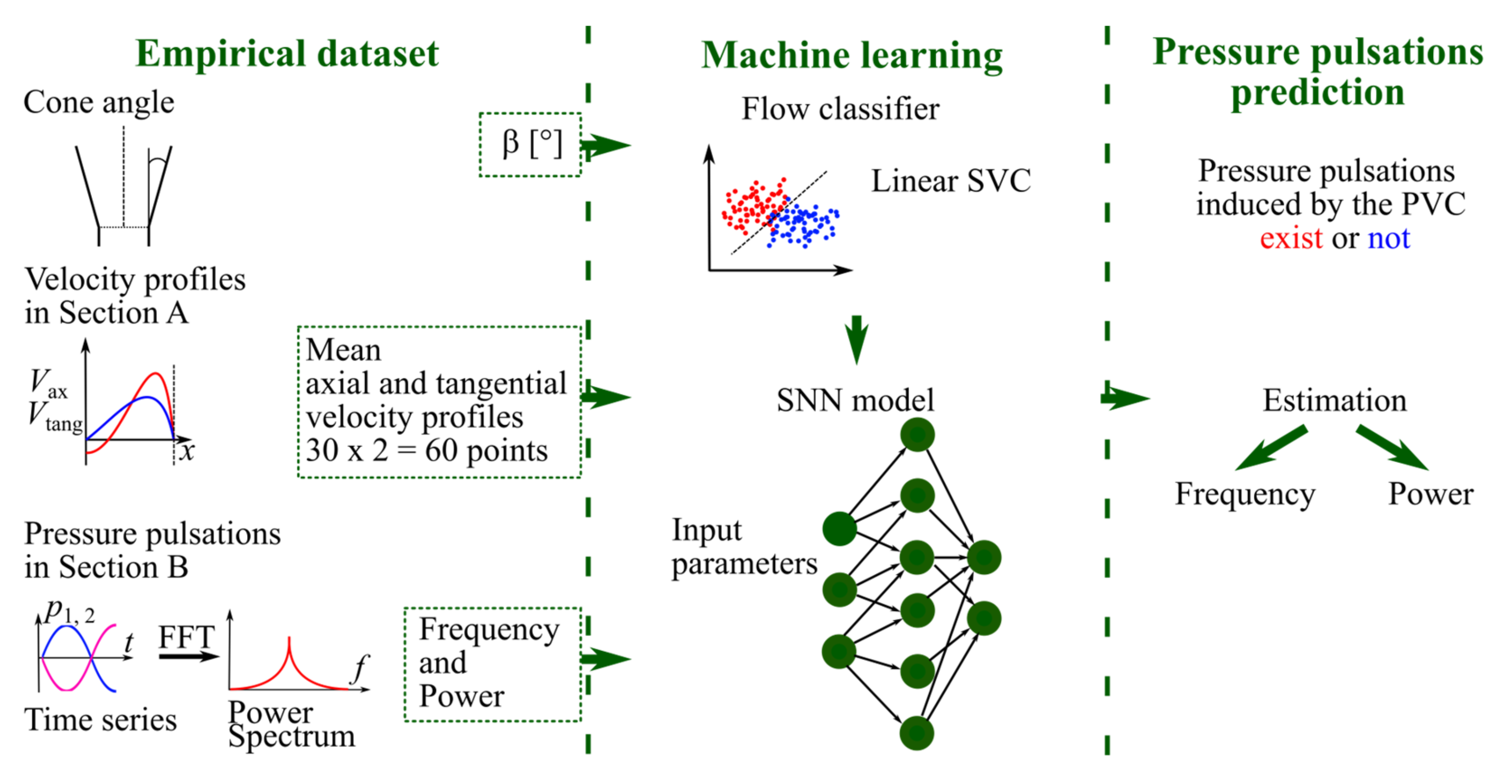
2.5. Empirical Database

The developed software allowed one to automatically vary the defining flow parameters (flow rate Q (Reynolds number Re) and angle of the guiding vanes α° (swirl number S)) with an acceptable accuracy. The half-angle of the conical diffuser β° was varied by selecting an ensemble of conical diffusers.

In the automated experiment, 1088 different regimes were measured (i.e., semi-profiles of the average velocity and the corresponding two pressure fluctuations signals). An analysis of the spectrograms of pressure fluctuation data showed that, for the opening angle β < 4°, the PVC inside the cone develops according to a different scenario. In this case, the power-frequency characteristics of the PVC depend on the output conditions of the cone, i.e., the sudden expansion conditions. In this regard, these regimes with β < 4° do not participate in further sampling in the analysis within the framework of machine learning and this article, but are of separate interest in terms of studying the swirling flows.

Table 1. Parameters of the empirical database.

Parameter	Parameter Range	Number of Regimes
Flow rate, Q [m3/h]	constant, 100	1
Angle of the guide vanes, α°	0–76.6	34
Cone angle, β°	4–15	12
Diaphragm, d [mm]	0 and 6	2
Total regimes involved in machine learning:	816

shows all the regimes and varied parameters of the accumulated empirical basis. Changes in the angle of the guide vanes α entailed a nonlinear change in the swirl number S according to Formula (1). The swirl number S was calculated separately for each regime.

For each regime in Table 1, semi-profiles of the average axial, and tangential components in the inlet section of the cone diffuser (in section A, Figure 1b) were obtained using LDA. Simultaneously with velocity measurements, the pressure fluctuation signals from two acoustic transducers p_1,2 were recorded (in section B, Figure 1b). All the accumulated experimental data were analyzed and reduced to a form suitable for machine learning algorithms. The mean value of the axial and tangential components was obtained for each measured velocity profile.

Figure 2 shows a characteristic spectrogram of the asynchronous mode of the pressure pulsations signal (p₁-p₂) for the diffuser with the angle β = 5°, and α varied within the range α = 40°–83°, where the PVC occurs in the flow. In the spectrogram, the PVC is illustrated by an emerging peak around 80–140 Hz when the value α increases, and therefore, the swirl number S, which overcomes its critical value, and the PVC occurs in the flow.

If we follow the power and frequency of the dominant peak (see Figure 3) corresponding to the PVC, we will see that the power and frequency increase with parameter α (swirl number S). In this case, the criterion for PVC formation is an important issue for classifying the flow and constructing a tool for predicting the PVC from the average velocity distributions. In this paper, a pressure pulsations level of 5% relative to the maximum pressure pulsations level in terms of signal power in a given conical diffuser was chosen to be such a selection criterion. This selection criterion was applied to the task of classifying the flow with respect to the PVC (present/absent).

The neural network-based prediction of the power-frequency characteristics of PVC was performed for an already marked database. The velocity profiles in the database classify the presence of the PVC. The regimes with a power lying below the threshold were not considered in further sampling.

According to Table 1, the Re number variation was excluded from consideration for further machine learning because, starting from approximately Re ≈ 30,000, the frequency response of the PVC becomes proportional to the flow rate of the medium (or the Re number). Figure 4 shows the Strouhal number Sh (the dimensionless frequency of the PVC) as a function of the rotational angle of the guide vanes α for three air flow rates Q = 60, 90, and 120 m³/h, which corresponds to three different Reynolds numbers Re = 23,600, 35,400, and 47,000. As it can be seen from the dependence reported above, for the two higher Re numbers, Sh is almost independent of Re. In this regard, the entire database has been measured at a fixed flow rate Q = 100 m³/h, which corresponds to Re = 39,000.

2.6. Machine Learning

Figure 5 shows the general concept of this study and the application of machine learning. Having a complete marked database, we proceed to the two tasks, namely to predicting the presence of PVC in the flow, and determining its frequency response of pressure fluctuations. Thus, the first model considered was a flow classifier based on the average velocity profiles, i.e., a tool for predicting the presence of PVCs in the flow. Several different ML algorithms were tested: Random Forest Classifier, SVC (Support Vector Classifier), Linear Support Vector Classification (Linear SVC), SGD (Stochastic Gradient Descent) Classifier, and K-Neighbors Classifier from the scikit-learn (Python) software package. The best accuracy was achieved with Linear SVC, an algorithm based on the support vector method. Based on this model, a classifier capable of predicting the PVC with high accuracy was created. The second model was designed for predicting the power-frequency characteristics of the flow when a PVC exists in it. In order to build the second model, we used the Self-Normalizing Neural Network (SNN) with five hidden layers: 1024, 512, 512, 256, and 16 neurons, respectively. The more detailed analysis included investigation and optimization of the network input parameters.

3. Results and Discussion

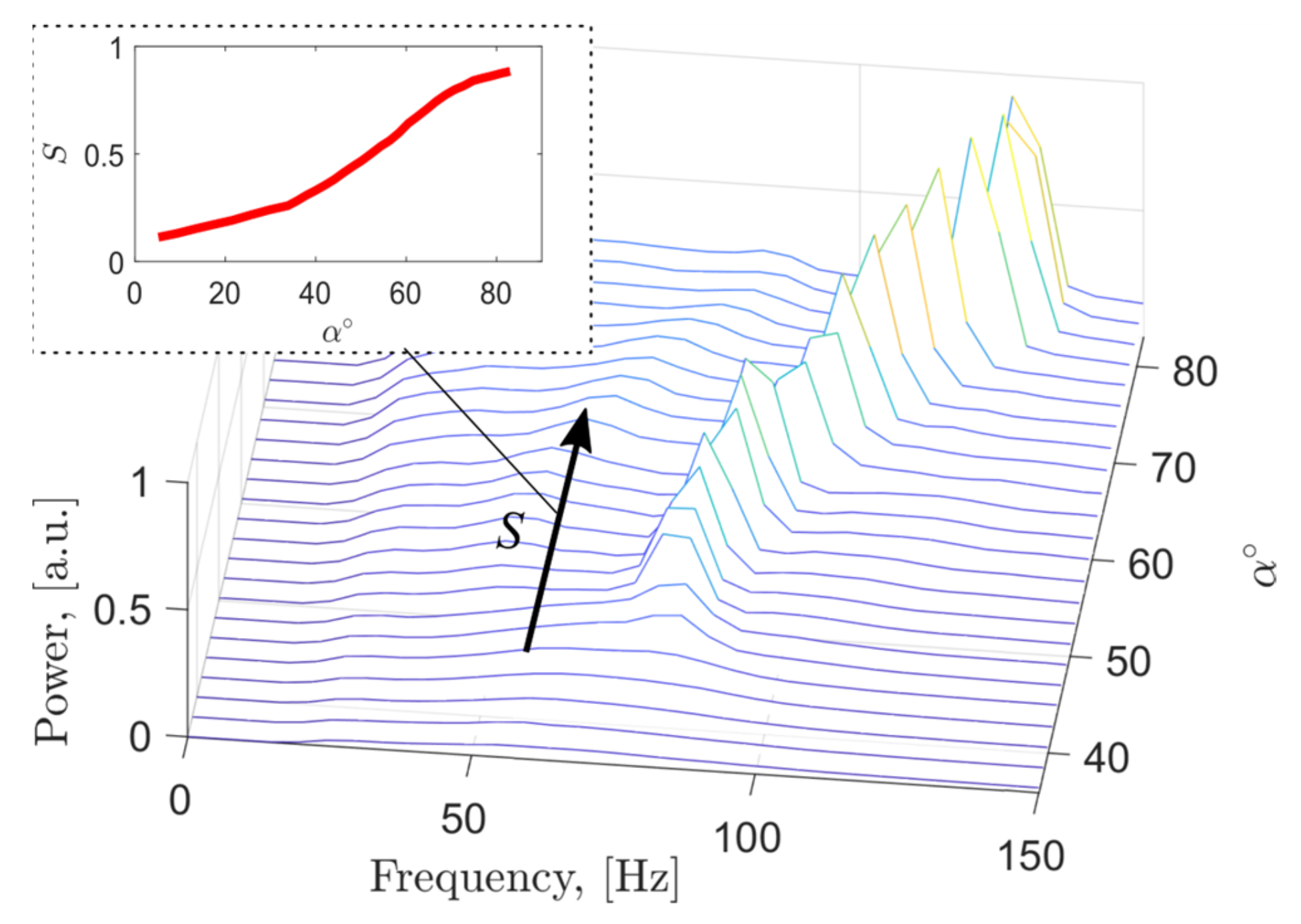
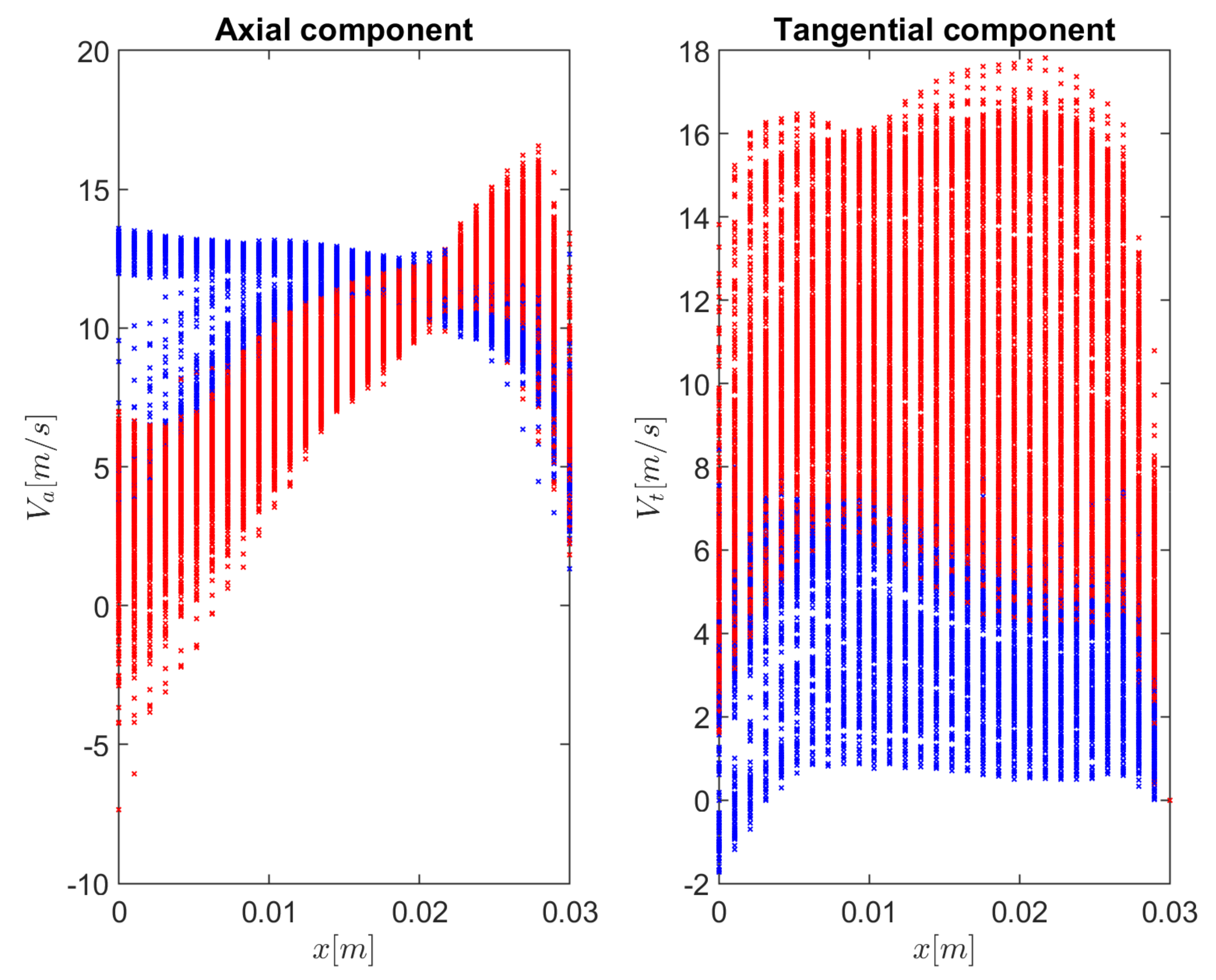
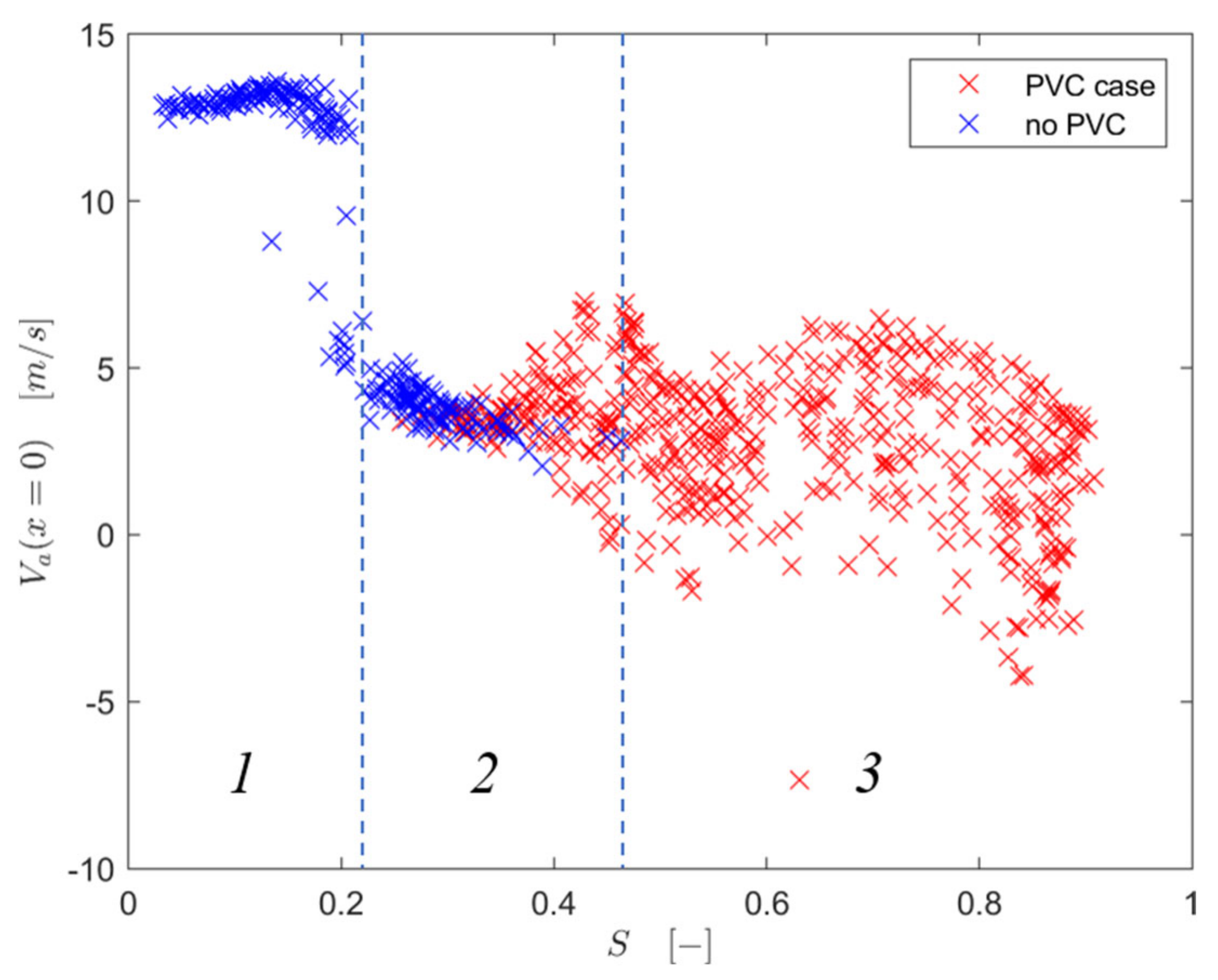
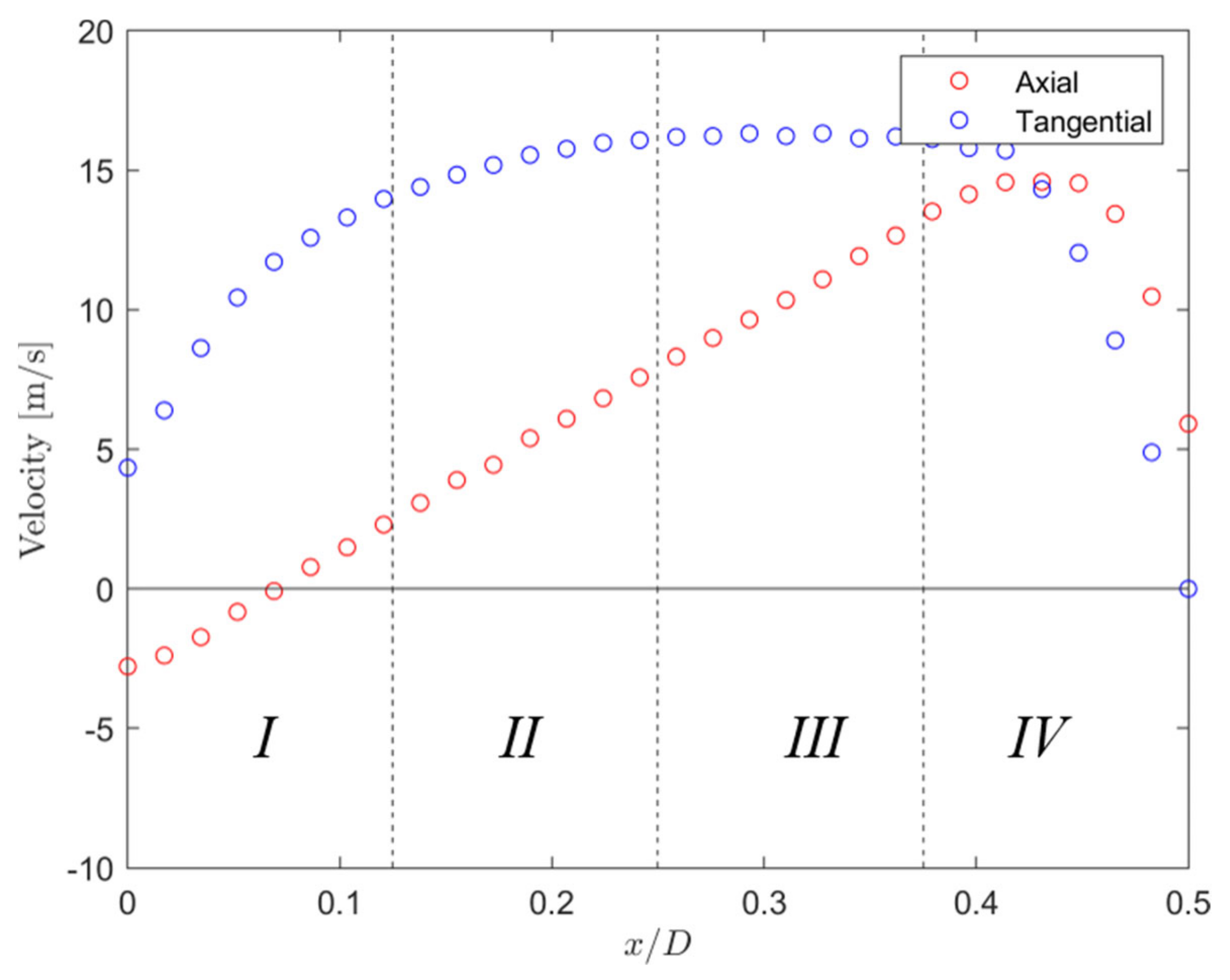
3.1. Flow Characteristics

An extensive series of automated experimental studies were performed, including measurements of the semi-profiles of the two velocity components and pressure pulsations in the swirling flow for the flow regimes summarized in Table 1. For each flow regime, the frequency and power of pressure pulsations were calculated from the pressure pulsations signals, and the PVC existence criterion (5% of maximum peak of the power in the spectra) was imposed.

All the measured distributions of the axial and tangential velocity components were plotted as an initial analysis of the velocity distributions and the regimes in which the PVC was registered (Figure 6). According to the processed pressure pulsations data, the red color indicates the velocity distributions in which PVC was detected in the flow, while the blue color indicates the velocity distributions in which no PVC was detected. It is possible to identify an area of intersection where the local velocity values fall into both the regions with and without PVC; however, it does not mean that the entire profile entirely belongs to both sets. This fact implies that considering only one velocity value at some local point along the radius would be insufficient for constructing a classifier of the flow with respect to the PVC formation, but one can see from the axial component that separation of the sets occurs near the diffuser axis.

From these considerations, Figure 7 shows the axial velocity V_a (x = 0) at the axis as a function of the swirl number S for all the analyzed flow regimes. The color shows whether the PVC is fixed in the flow or not. One can see that this representation makes a pretty clear distinction between the cases with and without PVC formation. Three characteristic regions of the swirl number can be observed; the raw data are grouped according to them. Region 1 corresponds to the low flow swirl numbers S, from 0 to 0.25; region 2 corresponds to the moderate swirl numbers from 0.25 to 0.55; region 3, to the strong swirl numbers S = 0.55 to 0.9. In region 2, axial velocity on the axis is nearly constant as the flow swirl number increases; however, once it reaches a value near S = 0.25, an abrupt jump in axial velocity and significant deficit of axial velocity are observed. The diagram shows that the PVC is not fixed in region 2. In region 2, the axial velocity on the axis starts to decrease monotonically, and the cases with PVC formation (red symbols) start to be recorded. Subsequently, as the swirl increases, the axial velocity decreases up to negative values due to formation of the central recirculation zone being characteristic of the PVC [52,63], and only the PVC-forming regimes are observed.

Nevertheless, the effect of varying the conical diffuser angle β is manifested in a different way within each region. In region 1, variations in the angle have almost no effect on velocity, while in regions 2 and 3, the increasing opening angle of the conical diffuser leads to monotonic reduction in velocity on the axis; the greatest effect is reached at the highest swirl numbers. The resulting findings indicate that the vortex decay region is sensitive even to small changes in the boundary conditions.

Therefore, the analysis of the empirical database clearly demonstrates that the axial velocity on the diffuser axis and the swirl number S can be used to construct a tool for predicting PVC according to the average velocity profiles.

3.2. The Classifier

The first task was to create a classifier that can predict the formation of the PVC with high accuracy according to the average velocity profiles at the diffuser inlet (Section A). The Linear SVC model from the Scikit-learn library was used for this task [64]. The Stochastic Gradient Descent (SGD) model showed similar results.

In order to train the ML model, the velocity distribution data were divided into training and test sets at a 7/3 ratio (573 and 243 samples, respectively). Grid search (GridSearch) was performed to select the optimal method parameters. Searching was performed according to the following hyperparameters summarized in

Table 2. Hyperparameters of the classifier model.

Hyperparameter Name	Range of Variation (Model Parameters with the Best Accuracy Are Underlined)
Penalty (the standard for determining the penalty)	l1, l2
Loss (loss function):	hinge, squared_hinge
Tol (tolerance parameter to stop training)	10−6, 10−5, 10−4, 10−3, 10−2
C (regularization parameter)	0.1, 0.25, 0.5, 0.75, 1.0
Max_iter (maximum number of learning iterations)	1000, 10,000

.

Figure 8 shows the classifier confidence diagram for the test dataset. It was possible to achieve 99% accuracy in determining the presence of PVC on the test dataset using this model.

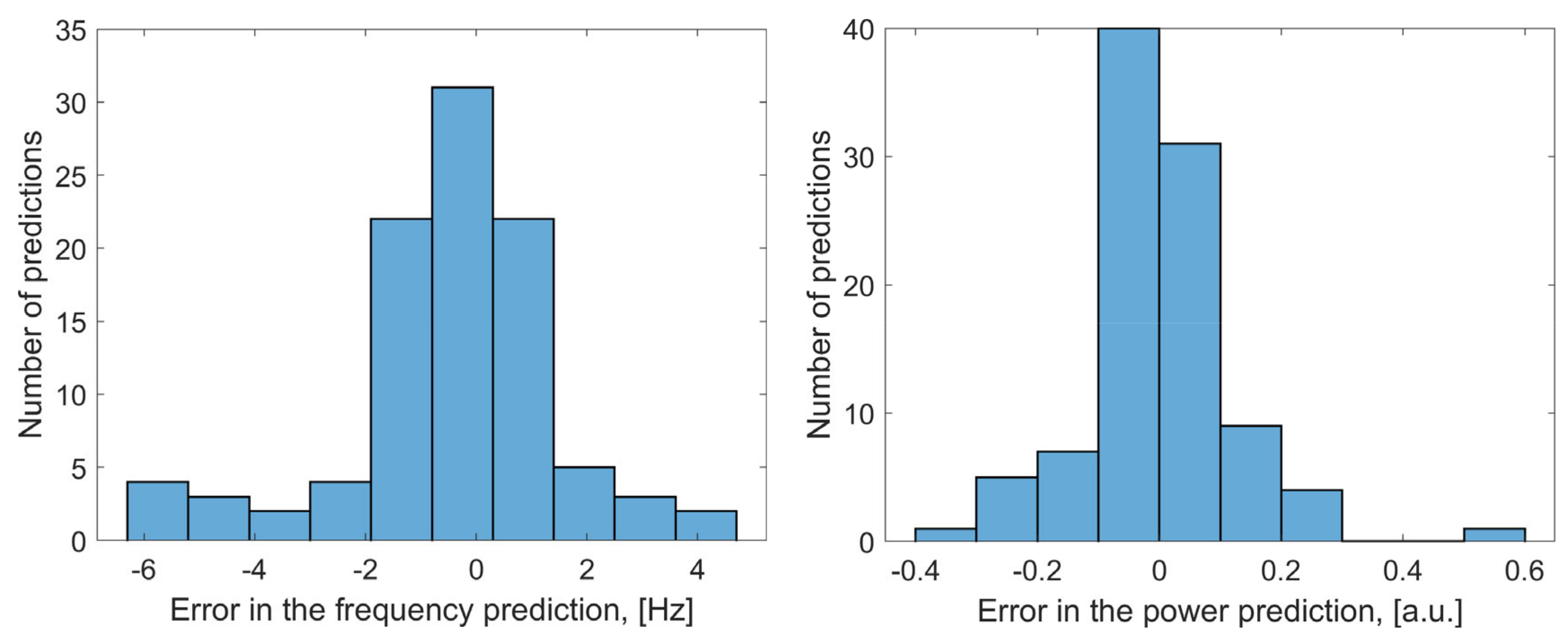
3.3. Self-Normalizing Neural Network (SNN)

The next task was to train a model that would be able to predict the power-frequency characteristics of pressure pulsations in the flow if the PVC existed. There were 61 parameters used as inputs: cone angle (β), axial, and tangential velocity values at 30 points.

For determining PVC frequency, SNN with five hidden layers was used: 1024, 512, 512, 256, and 16 neurons, respectively. In order to train the neural network, the dataset was divided into training, validation, and test sets at a 6/2/2 ratio (295, 98, and 98 samples). For determining the pressure pulsations power, a neural network with the same architecture was used. Figure 9 shows the distribution of errors in predicting the frequency and power of pressure pulsations using the SNN model. The final SNN errors are shown in

Table 3. Errors of the SNN model.

	Frequency of Pressure Pulsations	Power of Pressure Pulsations
Mean absolute percentage error (MAPE), %	1.01	5.40
Mean absolute error (MAE)	1.38	0.08

.

3.4. Feature Importance

To improve the interpretability of the ML model, a “feature importance” analysis was performed by comparing the coefficient measures of the learned SGD and Linear SVC models. For this purpose, the velocity profile was divided into four segments (I-IV) by radial coordinate x/D (see Figure 10). For each segment, the average velocity in this segment was calculated using the dimensionless x/D coordinate. A total of eight segment velocities (four segment velocities per velocity component) and the cone angle β were used to construct the model.

Figure 11 plots the most significant features of the two Linear SVC and SGD models for the flow classifier with respect to the PVC. The models show the same result in the following fact: the most important parameter in terms of predicting the PVC is the axial velocity component in the second quarter of the velocity profile (Ax-II). The Ax-II value can be interpreted as a certain tilt angle of the axial velocity profile whose variation would change the recirculation zone when the flow swirl increases, and is related to the formation of PVC in the flow (see Figure 10). The cone angle β is the second most important parameter highlighted by the model. The models somewhat diverge in the importance of other parameters.

The importance of features was also analyzed for determining the frequency and power of pressure pulsations. For this purpose, the model was analyzed using several methods implemented in the Captum library (in our case, Integrated Gradients, a neural network interpretation method in which integrated gradients are computed) [65]. For this approach, the dataset was prepared in the same way as for the classifier problem: eight average velocity values across segments (see Figure 10), and β values. All the values were normalized.

For the pressure pulsation frequency and power prediction problem, the MAPE was 1.23% and 2.78%, respectively. Figure 12 shows the importance diagrams of the Integrated Gradients method for predicting the power-frequency characteristics of pressure pulsations. It follows from the analysis that the most important features are the tangential velocity in the third quarter (Tang-II), which is responsible for the maximum value of the tangential velocity component, cone angle β, and axial velocity in the second quarter (Ax-II).

3.5. The Two-Parameter Model

Another approach was to use a limited number of input parameters as model inputs. Based on the above analysis, it is clear that the cone angle parameter β is important, and it is logical to take the integral swirl number S calculated from the average velocity profiles as the second parameter. The accuracy of predicting the frequency and power of pressure pulsations from the PVC by SNN learning was as follows (

Table 4. Errors of the two-parameter SNN model.

	Frequency	Power
Mean absolute percentage error (MAPE), %	2.68	6.38
Mean absolute error (MAE)	3.66	0.10

).

The decrease in accuracy expressed as relative percentage did not exceed 2% for determining the precession frequency, and 1% for determining the pulsations power. This fact emphasizes the importance of the flow swirl number, and the possibility of using it as one of the main flow-determining parameters. Figure 13 shows an example of successful application of a trained neural network to predict the precession frequency for five different swirl numbers in a conical diffuser with angle β = 9° using the full and two-parameter models.

Using the swirl number S can also be justified by the fact that, for example, with respect to flows in hydraulic turbines, there exist a number of semi-empirical models that allow one to calculate S with acceptable accuracy without measuring velocity profiles [66,67], thus making the ML tool for predicting unsteady flow characteristics even more versatile in the future.

4. Conclusions

An empirical database including the measured average input velocity profiles (the axial and tangential components), and emerging pressure pulsations in the swirling flow inside the cone diffuser was obtained. The unsteady vortex phenomenon PVC generated powerful pressure pulsations for some swirl regimes and the opening angle of the conical diffuser. In total, more than 10³ different flow regimes were measured by varying the swirl parameter and the opening angle of the diffuser. The following conclusions are drawn.

A flow classifier was constructed based on the resulting experimental data and the Linear SVC model. According to the average velocity profiles at the entrance to the cone diffuser, it allows one to predict the formation of the PVC phenomenon with high accuracy (99%).

It has been shown that it is possible to create a tool for predicting the frequency response of pressure pulsations of the flow in the presence of a PVC in a conical diffuser by constructing and training a regression artificial neural network SNN. The existence of the PVC can be predicted with high accuracy, and the frequency and power of pressure pulsations generated by the PVC can be determined according to the time-averaged input velocity profiles with an error being no more than 1.01% and 5.4%, respectively. It has been demonstrated using the two-parameter model that applying the cone diffuser angle and the integral swirl number as input parameters allows one to predict the power-frequency characteristics of the flow with an error of 2.7% and 6.4%, respectively.

If level of the pressure pulsations strongly depends on the site and method used for its registration, the frequency of pressure pulsations is a more universal value that is independent of the measurement site and method. Therefore, we can assume that the constructed neural network model is universal. Such a network can be applied to a wide class of technical devices with diffusive flow output. From the fundamental standpoint, this study is an attempt to systematize a wide class of swirling flows. An important relationship between the unsteady characteristics of the developed flow and the time-averaged input boundary conditions in the form of axial and tangential velocity distributions was revealed.

The authors believe the approach considered in the paper has great potential both in terms of practical applications for predicting the vortex frequency response of hydraulic turbines, and for developing fundamental theories of vortex structures.

References

1. Rheingans, W.J. Power Swings in Hydroelectric Power Plants. Trans. ASME 1940, 62, 171–184. [Google Scholar] [CrossRef]
2. Dörfler, P.; Sick, M.; Coutu, A. Flow-Induced Pulsation and Vibration in Hydroelectric Machinery: Engineer’s Guidebook for Planning, Design and Troubleshooting; Springer Science & Business Media: Berlin/Heidelberg, Germany, 2012. [Google Scholar]
3. Goyal, R.; Gandhi, B.K. Review of Hydrodynamics Instabilities in Francis Turbine during Off-Design and Transient Operations. Renew. Energy 2018, 116, 697–709. [Google Scholar] [CrossRef]
4. Kumar, S.; Cervantes, M.J.; Gandhi, B.K. Rotating Vortex Rope Formation and Mitigation in Draft Tube of Hydro Turbines—A Review from Experimental Perspective. Renew. Sustain. Energy Rev. 2021, 136, 110354. [Google Scholar] [CrossRef]
5. Fanelli, M. The Vortex Rope in the Draft Tube of Francis Turbines Operating at Partial Load: A Proposal for a Mathematical Model. J. Hydraul. Res. 1989, 27, 769–807. [Google Scholar] [CrossRef]
6. Nicolet, C.; Zobeiri, A.; Maruzewski, P.; Avellan, F. Experimental Investigations on Upper Part Load Vortex Rope Pressure Fluctuations in Francis Turbine Draft Tube. Int. J. Fluid Mach. Syst. 2011, 4, 179–190. [Google Scholar] [CrossRef] [Green Version]
7. Yamamoto, K.; Müller, A.; Favrel, A.; Landry, C.; Avellan, F. Pressure Measurements and High Speed Visualizations of the Cavitation Phenomena at Deep Part Load Condition in a Francis Turbine. IOP Conf. Ser. Earth Environ. Sci. 2014, 22, 022011. [Google Scholar] [CrossRef]
8. Skripkin, S.; Tsoy, M.; Shtork, S.; Hanjalić, K. Comparative Analysis of Twin Vortex Ropes in Laboratory Models of Two Hydro-Turbine Draft-Tubes. J. Hydraul. Res. 2016, 54, 450–460. [Google Scholar] [CrossRef]
9. Wahl, T.L. Draft Tube Surging Times Two: The Twin Vortex Phenomenon. Hydro Rev. States 1994, 8, 60–69. [Google Scholar]
10. Müller, A.; Favrel, A.; Landry, C.; Avellan, F. Fluid–Structure Interaction Mechanisms Leading to Dangerous Power Swings in Francis Turbines at Full Load. J. Fluids Struct. 2017, 69, 56–71. [Google Scholar] [CrossRef]
11. Alekseenko, S.V.; Kuibin, P.A.; Shtork, S.I.; Skripkin, S.G.; Tsoy, M.A. Vortex Reconnection in a Swirling Flow. JETP Lett. 2016, 103, 455–459. [Google Scholar] [CrossRef]
12. Minakov, A.; Sentyabov, A.; Platonov, D.; Dekterev, A.; Gavrilov, A. Numerical Modeling of Flow in the Francis-99 Turbine with Reynolds Stress Model and Detached Eddy Simulation Method. J. Phys. Conf. Ser. 2015, 579, 12004. [Google Scholar] [CrossRef] [Green Version]
13. Platonov, D.V.; Minakov, A.V.; Dekterev, D.A.; Maslennikova, A.V.; Kuibin, P.A. Experimental Observation of the Precessing-Vortex-Core Reconnection Phenomenon in a Combined-Flow Turbine. Tech. Phys. Lett. 2017, 43, 969–971. [Google Scholar] [CrossRef]
14. Susan-Resiga, R.; Muntean, S.; Tanasa, C.; Bosioc, A. Hydrodynamic Design and Analysis of a Swirling Flow Generator. In Proceedings of the 4th GRoWTH, Stuttgart, Germany, 12 June 2008. [Google Scholar]
15. Chigier, N.A.; Chervinsky, A. Experimental Investigation of Swirling Vortex Motion in Jets. J. Appl. Mech. 1967, 34, 443–451. [Google Scholar] [CrossRef]
16. Gupta, K.; Lilley, D.G.; Syred, N. Swirl Flows; Abacus Press: Kent, DC, USA, 1984. [Google Scholar]
17. Alligne, S.; Nicolet, C.; Tsujimoto, Y.; Avellan, F. Cavitation Surge Modelling in Francis Turbine Draft Tube. J. Hydraul. Res. 2014, 52, 399–411. [Google Scholar] [CrossRef]
18. Kuibin, P.A.; Okulov, V.L.; Susan-Resiga, R.F.; Muntean, S. Validation of Mathematical Models for Predicting the Swirling Flow and the Vortex Rope in a Francis Turbine Operated at Partial Discharge. IOP Conf. Ser. Earth Environ. Sci. 2010, 12, 012051. [Google Scholar] [CrossRef]
19. Susan-Resiga, R.; Dan Ciocan, G.; Anton, I.; Avellan, F. Analysis of the Swirling Flow Downstream a Francis Turbine Runner. J. Fluids Eng. 2006, 128, 177. [Google Scholar] [CrossRef]
20. Skripkin, S.; Zuo, Z.; Tsoy, M.; Kuibin, P.; Liu, S. Oscillation of Cavitating Vortices in Draft Tubes of a Simplified Model Turbine and a Model Pump–Turbine. Energies 2022, 15, 2965. [Google Scholar] [CrossRef]
21. Müller, J.; Sieber, M.; Litvinov, I.; Shtork, S.; Alekseenko, S.; Oberleithner, K. Prediction of Vortex Precession in the Draft Tube of a Model Hydro Turbine Using Mean Field Stability Theory and Stochastic Modelling. In IOP Conference Series: Earth and Environmental Science; IOP Publishing: Bristol, UK, 2021; Volume 774, p. 012003. [Google Scholar]
22. Pasche, S.; Avellan, F.; Gallaire, F. Part Load Vortex Rope as a Global Unstable Mode. J. Fluids Eng. 2017, 139, 051102. [Google Scholar] [CrossRef]
23. Muller, J.; Luckoff, F.; Kaiser, T.; Oberleithner, K. On the Relevance of the Runner Crown for Flow Instabilities in a Francis Turbine. In IOP Conference Series: Earth and Environmental Science; IOP Publishing: Bristol, UK, 2022; in press. [Google Scholar]
24. Minakov, A.; Platonov, D.; Litvinov, I.; Shtork, S.; Hanjalić, K. Vortex ropes in draft tube of a laboratory Kaplan hydroturbine at low load: An experimental and LES scrutiny of RANS and DES computational models. J. Hydraul. Res. 2017, 55, 668–685. [Google Scholar] [CrossRef] [Green Version]
25. Minakov, A.V.; Platonov, D.V.; Dekterev, A.A.; Sentyabov, A.V.; Zakharov, A.V. The Analysis of Unsteady Flow Structure and Low Frequency Pressure Pulsations in the High-Head Francis Turbines. Int. J. Heat Fluid Flow 2015, 53, 183–194. [Google Scholar] [CrossRef]
26. Zuo, Z.; Liu, S.; Liu, D.; Qin, D.; Wu, Y. Numerical Analyses of Pressure Fluctuations Induced by Interblade Vortices in a Model Francis Turbine. J. Hydrodyn. Ser B 2015, 27, 513–521. [Google Scholar] [CrossRef]
27. Galván, S.; Reggio, M.; Guibault, F. Numerical Optimization of the Inlet Velocity Profile Ingested by the Conical Draft Tube of a Hydraulic Turbine. J. Fluids Eng. 2015, 137, 071102. [Google Scholar] [CrossRef]
28. Faller, W.E.; Schreck, S.J. Neural Networks: Applications and Opportunities in Aeronautics. Prog. Aerosp. Sci. 1996, 32, 433–456. [Google Scholar] [CrossRef]
29. Grant, I.; Pan, X. An Investigation of the Performance of Multi Layer, Neural Networks Applied to the Analysis of PIV Images. Exp. Fluids 1995, 19, 159–166. [Google Scholar] [CrossRef]
30. Teo, C.; Lim, K.; Hong, G.; Yeo, M. A Neural Net Approach in Analyzing Photograph in PIV. In Proceedings of the 1991 IEEE International Conference on Systems, Man, and Cybernetics, Charlottesville, VA, USA, 13–16 October 1991; pp. 1535–1538. [Google Scholar]
31. Bishop, C.M.; James, G.D. Analysis of Multiphase Flows Using Dual-Energy Gamma Densitometry and Neural Networks. Nucl. Instrum. Methods Phys. Res. Sect. Accel. Spectrometers Detect. Assoc. Equip. 1993, 327, 580–593. [Google Scholar] [CrossRef]
32. Baldi, P.; Hornik, K. Neural Networks and Principal Component Analysis: Learning from Examples without Local Minima. Neural Netw. 1989, 2, 53–58. [Google Scholar] [CrossRef]
33. Milano, M.; Koumoutsakos, P. Neural Network Modeling for near Wall Turbulent Flow. J. Comput. Phys. 2002, 182, 1–26. [Google Scholar] [CrossRef] [Green Version]
34. Liu, Y.; Fang, Y. Predictive Control Strategy of Hydraulic Turbine Turning System Based on Bgnn Neural Network. In Proceedings of the International Symposium on Intelligence Computation and Applications, Wuhan, China, 19–21 December 2008; Springer: Berlin/Heidelberg, Germany, 2008; pp. 331–341. [Google Scholar]
35. Jambunathan, K.; Hartle, S.; Ashforth-Frost, S.; Fontama, V. Evaluating Convective Heat Transfer Coefficients Using Neural Networks. Int. J. Heat Mass Transf. 1996, 39, 2329–2332. [Google Scholar] [CrossRef]
36. Pierret, S.; Van den Braembussche, R. Turbomachinery Blade Design Using a Navier-Stokes Solver and Artificial Neural Network. In Turbo Expo: Power for Land, Sea, and Air; American Society of Mechanical Engineers: New York, NY, USA, 1998; Volume 78620, p. V001T01A002. [Google Scholar]
37. Abdurakipov, S.; Tokarev, M.; Pervunin, K.; Dulin, V. Modeling of the Tonal Noise Characteristics in a Foil Flow by Using Machine Learning. Optoelectron. Instrum. Data Process. 2019, 55, 205–211. [Google Scholar] [CrossRef]
38. Elsayed, K.; Lacor, C. Modeling, Analysis and Optimization of Aircyclones Using Artificial Neural Network, Response Surface Methodology and CFD Simulation Approaches. Powder Technol. 2011, 212, 115–133. [Google Scholar] [CrossRef]
39. Zhao, B.; Su, Y. Artificial Neural Network-Based Modeling of Pressure Drop Coefficient for Cyclone Separators. Chem. Eng. Res. Des. 2010, 88, 606–613. [Google Scholar] [CrossRef]
40. Gruber, P.; Farhat, M.; Odermatt, P.; Etterlin, M.; Lerch, T.; Frei, M. The Detection of Cavitation in Hydraulic Machines by Use of Ultrasonic Signal Analysis. Int. J. Fluid Mach. Syst. 2015, 8, 264–273. [Google Scholar] [CrossRef] [Green Version]
41. Hocevar, M.; Sirok, B.; Blagojevic, B.; Grabec, I. Experimental Modeling of a Cavitation Vortex in the Draft Tube of a Francis Turbine Using Artificial Neural Networks. J. Hydraul. Res. 2007, 45, 538–546. [Google Scholar] [CrossRef]
42. Hočevar, M.; Širok, B.; Blagojevič, B. Prediction of Cavitation Vortex Dynamics in the Draft Tube of a Francis Turbine Using Radial Basis Neural Networks. Neural Comput. Appl. 2005, 14, 229–234. [Google Scholar] [CrossRef]
43. Ahmed, S.A.; Raghavan, B.V. Free Vortex Turbulent Swirling Flow Reconstruction Using a Neural Network. In Proceedings of the Fluids Engineering Division Summer Meeting, American Society of Mechanical Engineers, Rio Grande, PR, USA, 8–12 July 2012; Volume 44755, pp. 783–788. [Google Scholar]
44. Raissi, M.; Perdikaris, P.; Karniadakis, G.E. Physics-Informed Neural Networks: A Deep Learning Framework for Solving Forward and Inverse Problems Involving Nonlinear Partial Differential Equations. J. Comput. Phys. 2019, 378, 686–707. [Google Scholar] [CrossRef]
45. Raissi, M.; Wang, Z.; Triantafyllou, M.S.; Karniadakis, G.E. Deep Learning of Vortex-Induced Vibrations. J. Fluid Mech. 2019, 861, 119–137. [Google Scholar] [CrossRef] [Green Version]
46. Véras, P.; Balarac, G.; Métais, O.; Georges, D.; Bombenger, A.; Ségoufin, C. Reconstruction of Numerical Inlet Boundary Conditions Using Machine Learning: Application to the Swirling Flow inside a Conical Diffuser. Phys. Fluids 2021, 33, 085132. [Google Scholar] [CrossRef]
47. Véras, P.; Métais, O.; Balarac, G.; Georges, D.; Bombenger, A.; Ségoufin, C. Reconstruction of Proper Numerical Inlet Boundary Conditions for Draft Tube Flow Simulations Using Machine Learning. Comput. Fluids 2023, 254, 105792. [Google Scholar] [CrossRef]
48. Brunton, S.L. Applying Machine Learning to Study Fluid Mechanics. Acta Mech. Sin. 2021, 37, 1718–1726. [Google Scholar] [CrossRef]
49. Liu, Z.; Favrel, A.; Miyagawa, K. Effect of the Conical Diffuser Angle on the Confined Swirling Flow Induced Precessing Vortex Core. Int. J. Heat Fluid Flow 2022, 95, 108968. [Google Scholar] [CrossRef]
50. Litvinov, I.V.; Sharaborin, D.K.; Shtork, S.I. Reconstructing the Structural Parameters of a Precessing Vortex by SPIV and Acoustic Sensors. Exp. Fluids 2019, 60, 139. [Google Scholar] [CrossRef]
51. Valera-Medina, A.; Syred, N.; Griffiths, A. Visualisation of Isothermal Large Coherent Structures in a Swirl Burner. Combust. Flame 2009, 156, 1723–1734. [Google Scholar] [CrossRef]
52. Litvinov, I.V.; Shtork, S.I.; Kuibin, P.A.; Alekseenko, S.V.; Hanjalic, K. Experimental Study and Analytical Reconstruction of Precessing Vortex in a Tangential Swirler. Int. J. Heat Fluid Flow 2013, 42, 251–264. [Google Scholar] [CrossRef]
53. Alekseenko, S.V.; Kuibin, P.A.; Okulov, V.L. Theory of Concentrated Vortices: An Introduction; Springer Science & Business Media: Berlin/Heidelberg, Germany, 2007; Volume 1, ISBN 978-3-540-73376-8. [Google Scholar]
54. Cassidy, J.J.; Falvey, H.T. Observations of Unsteady Flow Arising after Vortex Breakdown. J. Fluid Mech. 1969, 41, 727–736. [Google Scholar] [CrossRef]
55. Chanaud, R.C. Observations of Oscillatory Motion in Certain Swirling Flows. J. Fluid Mech. 1965, 21, 111–127. [Google Scholar] [CrossRef]
56. Alekseenko, S.V.; Kuibin, P.A.; Okulov, V.L.; Shtork, S.I. Helical Vortices in Swirl Flow. J. Fluid Mech. 1999, 382, 195–243. [Google Scholar] [CrossRef]
57. Skripkin, S.; Suslov, D.; Litvinov, I.; Gorelikov, E.; Tsoy, M.; Shtork, S. Comparative Analysis of Air and Water Flows in Simplified Hydraulic Turbine Models. J. Phys. Conf. Ser. 2022, 2150, 012001. [Google Scholar] [CrossRef]
58. Litvinov, I.; Gorelikov, E.; Shtork, S. Frequency Response of the Flow in a Radial Swirler. J. Mech. Sci. Technol. 2022, 36, 2397–2402. [Google Scholar] [CrossRef]
59. Tropea, C.; Yarin, A.L.; Foss, J.F. Springer Handbook of Experimental Fluid Mechanics; Springer: Berlin/Heidelberg, Germany, 2007; Volume 46, ISBN 978-3-540-25141-5. [Google Scholar]
60. Yanta, W.J.; Smith, R.A. Measurements of Turbulence-Transport Properties with a Laser Doppler Velocimeter. In Proceedings of the 11th Aerospace Sciences Meeting, American Institute of Aeronautics and Astronautics, Washington, DC, USA, 10–12 January 1973. AIAA Paper 73–169. [Google Scholar]
61. Cala, C.E.; Fernandes, E.C.; Heitor, M.V.; Shtork, S.I. Coherent Structures in Unsteady Swirling Jet Flow. Exp. Fluids 2006, 40, 267–276. [Google Scholar] [CrossRef]
62. Goyal, R.; Cervantes, M.J.; Gandhi, B.K. Characteristics of Synchronous and Asynchronous Modes of Fluctuations in Francis Turbine Draft Tube during Load Variation. Int. J. Fluid Mach. Syst. 2017, 10, 164–175. [Google Scholar] [CrossRef]
63. Yazdabadi, P.A.; Griffiths, A.J.; Syred, N. Characterization of the PVC Phenomena in the Exhaust of a Cyclone Dust Separator. Exp. Fluids 1994, 17, 84–95. [Google Scholar] [CrossRef]
64. Pedregosa, F.; Varoquaux, G.; Gramfort, A.; Michel, V.; Thirion, B.; Grisel, O.; Blondel, M.; Prettenhofer, P.; Weiss, R.; Dubourg, V.; et al. Scikit-Learn: Machine Learning in Python. J. Mach. Learn. Res. 2011, 12, 2825–2830. [Google Scholar]
65. Sundararajan, M.; Taly, A.; Yan, Q. Axiomatic Attribution for Deep Networks. In Proceedings of the International Conference on Machine Learning, Sydney, Australia, 6–11 August 2017; pp. 3319–3328. [Google Scholar]
66. Favrel, A.; Pereira, J.G., Jr.; Landry, C.; Müller, A.; Nicolet, C.; Avellan, F. New Insight in Francis Turbine Cavitation Vortex Rope: Role of the Runner Outlet Flow Swirl Number. J. Hydraul. Res. 2017, 56, 367–379. [Google Scholar] [CrossRef]
67. Skripkin, S.; Tsoy, M.; Kuibin, P.; Shtork, S. Swirling Flow in a Hydraulic Turbine Discharge Cone at Different Speeds and Discharge Conditions. Exp. Therm. Fluid Sci. 2019, 100, 349–359. [Google Scholar] [CrossRef]
Figure 1. The experimental setup: a sketch (a) and the measurement scheme (b).
Energies 16 02108 g001aEnergies 16 02108 g001b
Figure 2. Spectrogram of asynchronous mode of pressure pulsations with varied rotation angle α (which corresponds to swirl number S) in a conical diffuser with angle β = 5° (in the insert swirl number as function of α°).
Energies 16 02108 g002
Figure 3. The normalized power and frequency of the wall-measured pressure pulsations caused by PVC as functions of angle α (swirl number S) in a conical diffuser with angle β = 5°.
Energies 16 02108 g003
Figure 4. The Strouhal parameter Sh as a function of the angle of the guide vanes α at different Reynolds numbers Re in a conical diffuser with angle β = 5°.
Energies 16 02108 g004
Figure 5. Machine learning diagram of the empirical sample.
Energies 16 02108 g005
Figure 6. Illustration of all the measured semi-profiles of the axial and tangential component of the average velocity (the regimes with PVC according to the criterion are shown in red; the regimes without PVC are shown in blue).
Energies 16 02108 g006
Figure 7. Axial velocity component in the center of the diffuser (x = 0) for all the implemented flow regimes depending on the swirl number S (the regimes with PVC according to the selection criterion are shown in red; the regimes without PVC are shown in blue).
Energies 16 02108 g007
Figure 8. The confusion matrix of the PVC classifier.
Energies 16 02108 g008
Figure 9. Error histogram of the SNN model predicting the frequency (left) and power of pressure pulsations induced by the PVC (right).
Energies 16 02108 g009
Figure 10. Partitioning the velocity profile into segments for feature analysis. (The regime is β = 5° and α = 70°).
Energies 16 02108 g010
Figure 11. Histograms of feature importance for the SGD (left) and Linear SVC models (right).
Energies 16 02108 g011
Figure 12. Visualization of the importance of features in the frequency (left) and the power (right) of the pressure pulsations prediction task.
Energies 16 02108 g012
Figure 13. The results of applying the neural network model to the angle β = 9°.
Energies 16 02108 g013