Effect of Macroscopic Turbulent Gust on the Aerodynamic Performance of Vertical Axis Wind Turbine

Abstract

Vertical Axis Wind Turbines (VAWTs) have proven to be suitable for changing wind conditions, particularly in urban settings. In this paper, a 2D URANS (Unsteady Reynolds-Averaged Navier Stokes) numerical analysis is employed for an H-Darrieus VAWT. A turbulent domain is created through systemically randomising the inlet velocity to create macro-turbulence in front of the VAWT. The parameters for spatial and temporal randomisation of velocity and its effects on the turbine performance are studied for a mean free stream velocity, U_∞ = 10 m/s, and a tip speed ratio (TSR) of 4.1. The mean Coefficient of power (C_p) for randomised fluctuation of 2 m/s and half-cycle randomisation update frequency is 0.411 and for uniform inlet velocity is 0.400. The C_p vs. Tip Speed ratio plot suggests that the optimal tip speed ratio for operation is around 4.1 for this particular wind turbine of diameter 1 m, chord 0.06 m, and NACA 0018 airfoils. The effect of randomisation for tip speed ratio λ = 2.5, 3.3, 4.1, and 5.3 on the performance of the turbine is studied. Turbine wake recovers at a faster rate for macro-turbulent conditions and is symmetric when compared to wake generated by uniform velocity inlet. The maximum velocity deficit for a distance behind the turbine, x/d = 8 at TSR (λ) = 4.1 is 46% for randomised inlet and 64% for uniform inlet. The effect of randomisation for λ = 2.5 to 5.3 on the performance of the turbine is analysed. A time-varying gust based on International Electrotechnical Commission (IEC) Extreme Operating Gust is used to study the effect of fluctuating wind conditions in a turbulent environment. Since real-time conditions often exceed gust factors mentioned by IEC, winds with large gust factors such as 1.50, 1.64, and 1.80 are analysed. With an increase in gust amplitude, U_gust = 6 m/s to U_gust = 12 m/s on a free stream velocity of U∞ = 10 m/s, the mean C_p decreases from 0.41 to 0.35 since the wind turbine operates under tip speed ratios outside optimal range due to large fluctuations in incoming velocity.

1. Introduction

The recent trend in environmental degradation and climate change has led to a pressing need to shift towards renewable and sustainable sources of energy. With wind energy steadily gaining pace, the global wind energy market continues to be stable with about 591 GW in 2018, and approximately 51 GW installed worldwide every year. There has been an approximate 400% increase in power generated by wind turbines from 2008 to 2018 [1]. Though there are efficient methods to harness wind energy using large wind farms and offshore sites, there is still a void in the development of effective harnessing methods for urban conditions.

Unlike wind conditions in large wind sites, the urban winds are mainly characterised by unsteadiness in wind velocity and wind direction and have high turbulence intensity due to the interaction of winds with various physical obstacles such as buildings and trees, and localised temperature variations. Emejeamara et al. [2] measured wind velocities in urban environments and reported the presence of gustiness in urban winds and the need for their consideration in urban wind studies.

For energy extraction in large wind farms, conventional Horizontal Axis Wind Turbines (HAWT) are efficient choices. However, HAWTs do not prove to be as efficient as Vertical Axis Wind Turbines (VAWT) in urban areas. The power produced by HAWTs drops significantly when the direction of the wind changes, while that of the Vertical Axis Wind Turbines (VAWTs) remains constant irrespective of the directional change. VAWTs pose an advantage over HAWTs in urban conditions due to their omnidirectional characteristic [3,4,5]. As the angle of wind changed from 0° to 45° incident to HAWT, the voltage produced by the generator of wind turbines significantly dropped, according to Ishugah et al. [6]. Voltage further dropped to 0 V when the angle reached 90°. VAWTs, however, produced a steady voltage for all angles. When compared to a HAWT, a VAWT is suitable for urban environments because of less space requirement and more potential to produce power for the same swept area of the turbine [6]. VAWTs also have several other advantages over HAWTs due to their capability to operate at low tip speed ratios (TSR), low noise levels and ease of construction and maintenance, and thus are suitable choices for urban wind conditions [3,7,8].

In recent years, several kinds of research and analyses have been conducted on the performance and design of the VAWTs under various wind conditions. Many studies have focused on the effect of unsteady and fluctuating winds [9,10,11,12,13,14,15,16,17,18,19], impact of gust [20,21,22,23,24,25,26], and turbulence [27,28] on the performance of VAWTs.

Both numerical and experimental studies have been performed on the effects of unsteady winds on the performance of VAWTs. Danao et al. [18] experimentally studied these effects by employing 7% and 12% velocity amplitude fluctuations on a sinusoidal wind profile for a scaled wind tunnel model of a VAWT. Shahzad et al. [29] studied the effect of accelerating and decelerating airflow on VAWTs by steadily increasing the velocity from 4 m/s to 10 m/s and decreasing it back to 4 m/s. They established that even though the rate of acceleration is constant during acceleration and deceleration, their effects on VAWTs vary. Bhargav et al. [14] and Danao et al. [17] have numerically studied the performance dependency of the unsteadiness of the wind by establishing a relation between the wind velocity fluctuation amplitude and the fluctuation frequency. The fluctuating wind varies its velocity sinusoidal, and different analyses are performed by varying the fluctuation amplitude and frequency. These studies show that, as the fluctuation amplitude increases, the coefficient of power (C_p) values decreases significantly, and as the fluctuation frequency increases, the C_p value increases. Jafari et al. [30] used a wind model that generates quasi unsteady wind velocity by generating random velocities using the turbulence intensity of the wind, which was 20% in their study.

Studies comparing the computationally modelled sinusoidal wind and real-time unsteady winds have also been conducted. In a comparison study performed by Wekesa et al. [12], the performance results obtained computationally were compared to the empirically obtained results at specified locations, namely Marsabit and Garissa. Numerically obtained power densities of wind compared closely with the empirically obtained ones and had only marginal errors of 4% and 17%, respectively, at Marsabit and Garissa.

Gust winds are the winds with a sudden increase in wind speed, followed by a decrease in wind speed. The incoming winds, based on the direction, are classified into longitudinal, lateral, and upward [21]. Lee et al. [31] studied the influence of the vertical wind on the performance of a small vertical-axis wind turbine installed on the rooftop of a building and concluded that if the horizontal wind is greater than 8 m/s, the impact of the vertical wind and the impact of horizontal wind on the power output of the turbine is reduced.

The Extreme Operating Gust (EOG) standardised by the International Electrochemical Commission’s (IEC) [32] is used in this paper. EOGs are constituted by a decrease, followed by a steep rise, a steep drop, and a rise back to the original wind speed value. There has been research on the effects of gust winds on VAWTs. Onol and Yesilyurt [23] studied the effect of the IEC’s model of EOG on VAWTs through 2D URANS-based numerical simulations by plotting the power coefficient against the angle of attack for various Tip Speed Ratios. Wu et al. [20] studied the responses of VAWTs to lateral gustiness of wind using sinusoidal wind signals. They stated that gust influences are not only present in the immersion period but also in a much broader influencing period because of the mutual aerodynamic interaction between the gusts and rotor.

Even though the IEC has standardised gusts, several studies [22,33] have been performed comparing the original gust data and possible corrections that have to be made to the model to make it more accurate. Rakib et al. [22] compared the IEC 61400-2013 gust model to actual wind data for a 5 kW Aerogenesis turbine at Callaghan. It was observed that the average gust factor of experimental data was 26% higher and the rise-and-fall time was 21% shorter when compared to the IEC gust model. The frequency of occurrence of gust was also higher than the predictions by IEC. Thus, an increase in the mean amplitude of gust velocity, shorter rise, and fall time, and an increase in gust factor must be incorporated into the inlet gust model. The analyses on gust winds did not take into consideration the high turbulence levels in urban winds.

In order to reproduce the real-life turbulent urban wind conditions in numerical simulations, Balduzzi et al. [27] developed a numerical strategy for an unsteady RANS approach to generate macro-turbulence for wind energy applications. The study introduced macro-turbulence by spatially randomising the velocity values at the inlet. Further in the study, it was used to simulate the behaviour under turbulence of an H-Darrieus vertical axis wind turbine. The results produced by the simulations were also reported to match the experimental results.

The study of the wake is necessary for predicting aerodynamic behaviour downstream of the turbine. Extensive experimental and numerical studies on the effect of wind conditions on wake and wake characteristics of VAWTs are reported. Lam and Peng [34] studied wake characteristics of VAWT using 2D and 3D simulation models. They found that SST turbulence models are coherent with experimental results. Peng et al. [35] experimentally studied wake aerodynamics of a 5-straight-bladed VAWT through wind tunnel tests. They concluded that wake asymmetry was attributed to the larger number of vortices shed in the windward direction. In addition, a counter-rotating pair of vortices was found downstream that contributed to complete mixing and faster wake recoveries. Rezaeiha et al. [36] studied the effect of tip speed ratio on wake structures and its influence on wake parameters such as length of the turbine wake and velocity deficit.

The effect of macro-turbulence in winds and gustiness of winds on VAWTs has been separately studied in the past for a typical urban environment. However, VAWTs are likely to be installed in environments with wind profiles that have a super-imposition of both. Thus, this study analyses the effect that macro-turbulent gusty winds on the performance and wakes of VAWTs. In the current study, wind speeds are varied both spatially and temporally in an attempt to reproduce a typical urban setting under an Extreme Operating Gust (EOG) criteria. The temporal randomisation accounts for the unsteadiness in wind velocities, and spatial randomisation attempts to reproduce non-homogeneous eddies with larger length scale as present in urban winds. This work studies inlet randomisation parameters such as randomised fluctuation and randomisation update frequency on a steady inlet velocity and its effects on the upwind conditions and performance of the VAWT. It includes the effect of Tip Speed Ratio (TSR) on the performance of the VAWT and a study of wake turbine characteristics for different tip speed ratios for randomised inlet conditions. A comparison of uniform and randomised velocity inlet cases on turbine performance and wake is performed. The effect of gust parameters such as gust amplitude and gust time period are also studied for spatially randomised time-varying gust cases.

2. Problem Statement

The present study uses a 2-dimensional simulation of a 2-bladed H type VAWT with NACA0018 aerofoil. The height and diameter of the turbine are both equal to 1 m, and solidity (σ) is 0.12(σ = Nc/D). The shaft diameter (D) is 0.04 m, and the chord length of the aerofoil (c) is 0.06 m. N signifies the number of blades. The effect of struts is disregarded in this study.

Table 1. Geometric features of the turbine considered for the study.

Axis of Rotation	Vertical
Blade profile	NACA 0018
Chord, c	0.06 m
Diameter of rotor	1 m
Frontal area of the rotor	1 m2
Solidity, σ	0.12
Number of blades	2

shows the geometric features of the turbine considered for the study.

Urban wind conditions are non-uniform spatially. Hence it is essential to understand the performance of the VAWT with spatially varying macro-turbulence.

The urban winds are mainly characterised by their gustiness, unsteadiness in wind velocity and direction, and high turbulence levels. Unlike the wind flow in an open wind farm, the wind in urban regions will have to make its way around significantly denser tall structures such as buildings and poles. This leads to a flow that is non-homogeneously filled with eddies of large length scales, which result in a ‘macro-turbulent’ wind flow. The velocity contour of such a macro-turbulent inflow is presented in Figure 1a. Along with the local fluctuations of wind speeds caused by urban structures, one can observe larger and characteristic fluctuations in the freestream velocity of the wind result. The International Electrotechnical Commission (IEC) has characterised different types of such fluctuations and one such wind fluctuation, characterised by sudden rise and fall of wind speeds, is an Extreme Operating Gust (EOG), represented by the velocity plot in Figure 1b. With gusts being a fairly common wind phenomenon, urban environments are also susceptible to them. Therefore, in an urban environment, one can observe local winds with smaller and high frequency velocity fluctuations compounded with larger and low frequency variations in wind due to gusts. Inflow wind speed, averaged over the frontal area of a VAWT rotor subjected to such gusty wind conditions, can be best represented by the black coloured plot of wind velocity in Figure 1b. These characteristics of urban winds are detrimental to both the performance and structural integrity of VAWTs. Though significant research has been performed on studying the effects of gusts on the performance of VAWTs, the local unsteadiness and turbulent nature of urban winds have been undermined. Thus, the focus of the present study is to analyse the effects of unsteady, macro-turbulent gusty winds on the performance of VAWTs. Randomisation has been performed spatially (Figure 1a) and temporally (Figure 1b) to account for unsteadiness in wind velocity and turbulence levels, respectively.

3. Numerical Methodology

The simulations were carried out in commercial CFD package ANSYS Fluent 19.2. The flow is considered to be incompressible, as the velocity is negligible compared to the sonic speed. The flow is solved using incompressible 2D Unsteady Reynolds Averaged Navier Stokes (URANS)-based 4 equation transition SST model. The equations of conservation of mass and momentum solved for modelling the flow are given in Equations (1) and (2):

$$\nabla ·\overrightarrow{v}=0$$

(1)

$$\nabla ·\left(\overrightarrow{v}\overrightarrow{v}\right)=-\nabla p+\nabla ·\left(\overline{\overline{\tau }}\right)+\rho \overrightarrow{g}$$

(2)

$$\overline{\overline{\tau }}=\left(\mu +{\mu }_t\right)\left[\nabla \overrightarrow{v}+{\left(\nabla \overrightarrow{v}\right)}^T-\frac{2}{3}\nabla .\overrightarrow{v}I\right]$$

(3)

where $\rho$ is the density [kg/m³], $\overrightarrow{v}$ is the velocity [m/s], $\overrightarrow{g}$ is the acceleration due to gravity [m/s²], p is the pressure [Pa], $\overline{\overline{\tau }}$ is the stress tensor [N/m²], μ is the dynamic viscosity [N m²/s], μ_t is the turbulent viscosity [m²/s] closed by a suitable turbulence model, and I is an identity matrix.

The equations used for modelling turbulence, i.e., the equations for transition SST model are given in Equations (4) and (5):

$$\frac{\partial \left(\rho \gamma \right)}{\partial t}+\frac{\partial \left(\rho U_j\gamma \right)}{\partial x_j}=P_{\gamma 1}-E_{\gamma 1}+P_{\gamma 2}-E_{\gamma 2}+\frac{\partial }{\partial x_j}\left[\left(\mu +\frac{{\mu }_t}{{\sigma }_y}\right)\frac{\partial \gamma }{\partial x_j}\right]$$

(4)

$$\frac{\partial \left(\rho {\overline{R\theta }}_{\theta t}\right)}{\partial t}+\frac{\partial \left(\rho U_j{\overline{R\theta }}_{\theta t}\right)}{\partial x_j}=P_{\theta t}+\frac{\partial }{\partial x_j}\left[\left(\mu +{\mu }_t\right)\frac{\partial {\overline{R\theta }}_{\theta t}}{\partial x_j}\right]$$

(5)

In a comparative study of turbulence models by Darcozy et al. [37], the k-epsilon Realisable and k-omega SST models provide accurate results in locating the optimal tip speed ratio value for a VAWT for a 2D CFD analysis of an H-Darrieus-type VAWT. However, in a study by Rezaeiha et al. [38], various turbulence models were compared for accuracy in modelling turbulence. The study concluded that SST-based models are best suited for URANS-based VAWT simulations and transitional SST models for simulations in which the flow transitions from laminar to turbulent. Since the present study is concerned about transitional flows in which the range of the Reynolds number is from 1.2 × 10⁶ to 2.0 × 10⁶, the transition SST turbulent model is chosen for the simulations.

For convective term discretisation, the second-order upwind scheme is used. The Coupled algorithm is employed for handling the pressure and velocity coupling. The double-precision segregated solver with an implicit method, was utilised for solving the discretised algebraic equations.

3.1. Wind Inlet Conditions

The inlet velocity is defined using a custom User-defined Function (UDF) in ANSYS FLUENT to reproduce desired turbulent flow conditions inside the computational domain. UDF allows direct interaction with the solver through customisation of inlet boundary conditions and execution for a specified number of iterations. The velocity values are randomised, both temporally and spatially. Temporal randomisation is performed to account for the unsteadiness of wind velocities in urban conditions and spatial randomisation for the high turbulent wind conditions in urban areas. The velocity values fed to the solver will be randomised by maintaining the integrity of the original wind data, i.e., the mean and standard deviation of the wind data before and after randomisation will be the same.

The gust signal chosen for the study is an IEC standardised extreme operating gust and the variation of velocity of wind with time follows the Equation (6):

$$V\left(t\right)=(0.37*A*\left(sin\left(3\pi t/T\right)\right)*\left(1-cos\left(2\pi t/T\right)\right)$$

(6)

where A and T are gust amplitude and time period.

Accounting for the unsteadiness of wind velocities in urban wind conditions, the wind signal is randomised temporally. This is achieved by adding random values, within the range of random velocity fluctuation, to the IEC standard gust profile. The temporal randomisation scheme discretises the IEC gust signal based on the desired randomisation update frequency. It adds fluctuation magnitude to the original magnitude of wind velocity. The resultant velocity will thus be a sum of the original gust velocity and a random fluctuation added within the range of specified velocity fluctuation. This randomisation is better expressed through the figures in Figure 1b. Uniform wind case (where the mean velocity is kept constant at 10 m/s) is also randomised using the same method. The chosen velocity fluctuation for randomising the IEC gust profile temporally is 6 m/s and the randomisation update frequency is 90.

The spatial randomisation randomises the wind data spatially by assigning different velocities to each of the nodes at the velocity inlet of the computational domain. Both the X and Y components of the velocity vectors will be randomised. The X component gets assigned by different velocities to each of the nodes at the inlet. The randomisation in the Y component of velocity helps in changing the direction of the velocity vector, thus introducing macro-turbulence.

3.2. Computational Domain and Grid

The computational analyses performed in this study employ the use of 2D computational domains for computational simplicity. Rezaeiha et al. [39] compared the results of 2D and 2.5D simulations for low solidity wind turbines and established that 2D simulation results show good agreement with experimental results. The study on the effectiveness of 2D analyses for straight-bladed Darrieus VAWTs by Bianchini et al. [40] showed that the results from 2D CFD analyses are significantly accurate and reliable upon considering the placement of lateral boundaries at a distance far enough to simulate an open-air flow field.

The computational domain, as illustrated in Figure 2a, consists of a rotating inner domain where the turbine is located and a fixed rectangular domain surrounding the core. To provide an idea about the turbine geometry in 3D, a representative image is shown in Figure 2b. For the computational purposes, we have considered a 2D cross-sectional plane of the turbine perpendicular to the axis of rotation and have not considered the struts connecting the blades to the shaft. A sliding interface is employed between the fixed domain, and the rotating core enables rotation of the turbine. The meshing of the computational domain has been performed using commercial software GAMBIT v2.4. The inner domain is dynamic and made to rotate at an angular velocity of 82 rad/s to simulate the rotation of the turbine. The diameter of the inner mesh (dc) is 2.5 m, and the dimensions of the outer domain are 45 m and 40 m along the length (di + do) and breadth (W), respectively. With reference to Rezaeiha et al. [39], the turbine is placed at a distance of 15 m from the inlet (di). The side AB of the domain is the spatially varying velocity inlet, side CD is the pressure outlet, and BC and CD of the domain are walls as shown in the Figure 2a.

The side AB of the domain is a spatially varying velocity inlet that is given velocity values by a UDF hooked to the CFD solver, side CD is the pressure outlet with 1 atm pressure, and BC and AD of the domain are no-slip walls as shown in Figure 2a. The blades have a no-slip wall boundary condition with 628 nodes and a grid length of 5 × 10⁻⁵ m with a growth factor of 1.22. The computational domain totally consists of around 0.8 million cells. The grid independence study is performed by comparing the turbulence intensity and the turbulent length scales acquired by running simulations in the present grid and a finer grid for both randomised velocity inlet cases. Figure 3a shows the refinement of the mesh downstream of the turbine for performing accurate wake studies. The blade angle is measured in a counter-clockwise direction, which forms the basis for choosing the time step interval. Figure 3b represents the rotating domain of the mesh, and Figure 3c shows the region around the blade that is finely meshed to analyse blade-flow interactions with better accuracy.

3.3. Computational Methodology

The explicit relaxation factors for momentum and pressure are both 0.75. The under-relaxation factors for turbulent kinetic energy, dissipation rate, and intermittency are 0.4. The residuals for convergence are 10⁻⁵ for the continuity equation and 10⁻³ for velocity, turbulent kinetic energy, dissipation rate, and other variables. Time step size is taken to be time taken by the rotor to complete 0.5° of rotation. The results are read during the cycles 60–120 turbine cycles for the steady mean velocity case at tip speed ratio (λ) of 4.1. For the IEC gust cases, the results are read 120–160 turbine cycles for gust time period 3 s, 120–200 turbine cycles for time periods 6 s, and 120–200 turbine cycles 10.5 s. This allows time for the gust signal to reach the turbine and enough time for proper wake study.

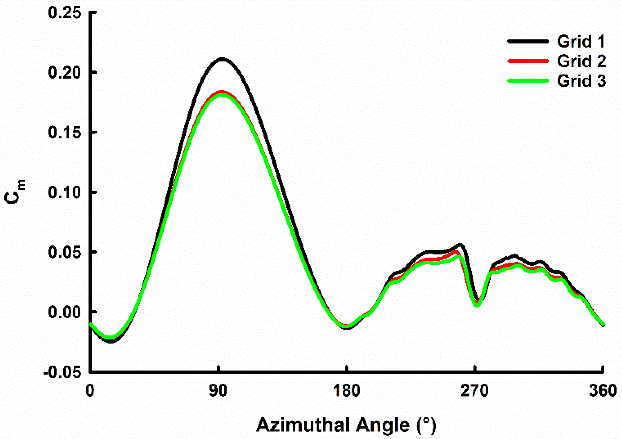
4. Validation and Grid Independence

For any results obtained by numerical simulation, validation is essential and mandatory for the results of the same to be considered for further analysis. The study involves a numerical analysis of vertical axis wind turbine. Hence, a validation against an experimental result is carried out. The CFD results of Rezaeiha et al. [36] and experimental results of Castelli et al. [41] are plotted against the CFD results obtained for a 3-bladed vertical axis wind turbine in Figure 4. It is found that at lower tip speed ratio, the numerical results are in line with the experimental results. This percentage of error is minimal. Grid independence is conducted by running three different grid cases with 0.4 million, 0.8 million, and 1.4 million grid points represented by grid 1, grid 2, and grid 3, respectively, in Figure 5. As the results given by grid 2 were at par with the results predicted by grid 3, which is almost double the grid points, it was decided to do the remaining set of simulations using grid 2.

5. Results and Discussion

The present study analyses the effect of inlet velocity randomisation parameters such as randomisation fluctuation and randomisation update frequency on the performance of a VAWT at a constant tip speed ratio of 4.1. The effect of Tip Speed Ratio on the coefficient of power and wake structure was studied. Further, the effect of gust parameters such as gust amplitude and gust time period for an IEC Extreme Operating Gust was investigated.

5.1. Effect of Randomisation Parameters on the VAWT Performance

5.1.1. Effect of Randomised Fluctuation

In Figure 6a, the variation of coefficient of power of the wind turbine due to the effect of randomised fluctuation of 2 m/s, 4 m/s, and 6 m/s at a constant tip speed ratio of 4.1 is shown. The randomised fluctuation magnitude is applied on an inlet mean velocity magnitude of 10 m/s. The value of C_p keeps fluctuating due to frequent updates of velocity at the inlet boundary, for every half rotation of the turbine. It is observed that as the randomisation fluctuation of velocity decreases from 6 m/s to 2 m/s, the mean value of C_p, represented by the dashed line, increases by a small margin of 0.01. This is because, for lower randomised fluctuations, the range of velocity values at all the inlet nodes is less compared to higher randomised fluctuations. For randomised fluctuation of 2 m/s, the velocity values vary from 12 m/s to 8 m/s, whereas for randomised fluctuation of 6 m/s, the velocity values vary from 16 m/s to 4 m/s. Since the velocities before the turbine could be of small magnitude in higher randomised fluctuation cases, the value of C_p produced is also low. The maximum and minimum bounds of C_p are represented by dotted lines in Figure 6a. The decrease in range values of C_p by 0.06 and a standard deviation of C_p by 0.01 from the randomised fluctuation of 6 m/s to 2 m/s is due to the same reason. The mean C_p values of cases with randomised inlet velocity are always higher than uniform velocity cases due to the effect of upstream macro-turbulence. The mean C_p value for randomisation fluctuation of 2 m/s is 0.411 and mean C_p for uniform velocity is 0.400 for λ = 4.1.

The effect of randomisation inlet velocity on the coefficient of power is shown in Figure 6b. It is noticed that as the mean free stream velocity varies, C_p follows a similar trend. There is a delay in C_p with respect to the free stream velocity through most peaks and troughs when plotted against flow time. The value of C_p increases as the magnitude of velocity in front of the turbine increases, and C_p drops as velocity magnitude decreases. As the magnitude of fluctuation of velocity increases, the time lag for C_p increases. It is also noticed that in regions with a higher frequency of fluctuation in velocity, the variation in C_p does not reflect the frequency of velocity fluctuation.

Figure 7 describes the variation of the Coefficient of Moment (C_m) for a single blade over an entire turbine rotation. In general, the C_m values peak at 90° where a dynamic stall occurs. During downwind conditions, a small variation in C_m is noticed and can be attributed to the interaction of blades with the wake created by the central shaft. There is a substantial variation in peak C_m values for different turbine cycles due to variation of wind velocity due to spatial randomisation and different randomised fluctuations of the inlet velocity. The range of peak C_m values is of higher magnitude for randomised fluctuation of 6 m/s (Figure 7a) than for randomised fluctuation of 2 m/s (Figure 7b).

5.1.2. Effect of Randomisation Update Frequency

The effect of update frequency of inlet profile for updates at every 45, 90,180, and 360 time-steps on the variation of C_p is studied. The tip speed ratio is maintained at 4.1, and the randomised fluctuation magnitude is 6 m/s on an inlet mean velocity magnitude of 10 m/s for all simulations. Figure 8a shows the variation of mean free stream wind velocity (U_∞) for all randomisation update frequency cases. The velocity values are taken at 0.75 d upstream of wind turbine and averaged over a width of 1.5 d. There is a decrease in the magnitude of fluctuation of wind velocity from an update frequency of 360 time-steps to 45 time-steps. The standard deviation of fluctuating velocity is 0.21 m/s for update frequency of 360 time-steps and 0.11 m/s for update frequency of 45 time-steps. The range of velocity fluctuation is 0.4 m/s higher in the case of update frequency of 360 time-steps compared to 45 time-steps. The flow field upstream of the turbine is more uniform for update frequency of 45 time-steps (Figure 8c) than for update frequency of 360 time-steps (Figure 8b), which is characterised by a higher magnitude of macro-turbulence. As the update interval decreases, the flow field in front of the turbine becomes uniform.

In Figure 9, it is observed that there are frequent C_p peaks in analysed data for an update frequency of 45 time-steps when compared to an update frequency of 360 time-steps. For cases of slower randomisation updates (update frequencies of 180 time-steps and 360 time-steps), the velocity at the inlet diffuses and becomes less spatially random by the time wind reaches the turbine. The effect of these velocities is prominent on the blade because of larger update intervals, and thus higher peaks and troughs of C_p are achieved. Thus, lower update frequencies such as 180 time-steps and 360 time-steps have a higher magnitude of fluctuations of C_p with respect to the mean C_p, hence larger values of the standard deviation of C_p, 0.24 and 0.28, respectively.

The range of variation of C_p is 0.11 for update frequency of 180 time-steps and 0.14 for the update frequency of 360 time-steps. On the contrary, the spatial randomness of velocity is maintained before the turbine for faster updates of 45 and 90 time-steps. The number of time-steps for the inlet wind is not sufficient to develop large fluctuations on C_p. Consequently, update frequencies of 45 and 90 time-steps produce C_p fluctuations of smaller magnitude closer to the mean C_p generated by the wind, i.e., the standard deviations of C_p are 0.12 and 0.16, respectively. The range of variation of C_p is 0.06 for update frequency of 45 time-steps and 0.07 for the update frequency of 90 timesteps. The fluctuations of the C_p value from the mean are highest in case of an update frequency of 360 time-steps and gradually decrease for quicker updates of 180, 90, and 45 time-steps.

Figure 10 shows the variation of the Coefficient of Moment (C_m) with respect to the azimuthal angle for a single blade. It is observed that the C_m plot follows a similar pattern in both update frequencies of 45 time-steps (Figure 10a) and 360 time-steps (Figure 10b) except at peak C_m values at 90° and downstream wake affected region after 180°.

5.2. Effect of Tip Speed Ratio on Coefficient of Power

The average wind velocity upstream of the turbine for tip speed ratios 2.5, 3.3, 4.1, and 5.3 is shown in Figure 11. Tip Speed ratio (λ) is the ratio between the rotational speed of the wind turbine and the free stream velocity. The mean wind velocity at the inlet for all cases is maintained at 10 m/s with a randomised fluctuation of 6 m/s; the rotational speed of the turbine varies with the tip speed ratio. As the wind approaches the turbine, it is noticed that with a decrease in tip speed ratio, the mean velocity of the wind increases, taken at 0.75 d upwind, and averaged over a width of 1.5 d (Figure 11a). Since the relative velocity of the turbine increases with the tip speed ratio, resistance due to turbine will increase, blocking the incoming wind. Hence, the mean velocity values are 9.48 m/s for λ = 2.5 and 8.56 m/s for λ = 5.3. The magnitude of fluctuation of velocity also decreases with an increase in the tip speed ratio. The standard deviation of fluctuating velocity is 0.30 m/s for λ = 2.5 and 0.20 m/s for λ = 5.3.

The dotted line in Figure 11a represents the uniform velocity condition, and the dashed line represents the mean of randomised velocity condition. The mean of randomised velocity is of similar value to the magnitude of uniform velocity. The mean of randomised velocity for λ = 2.5 is 9.48 m/s and 9.53 m/s for the uniform velocity case. The fluctuation of inlet velocity is also taken at 1 d upwind of the turbine and 1.25 d upwind of the turbine averaged over a width 1.5 d (Figure 11b). The velocity fluctuations follow a similar variation for all tip speed ratios at the three upwind locations. As the distance from the turbine decreases, the mean of randomised velocity also decreases. The mean of randomised velocity for λ = 2.5 is 9.69 m/s at 1.25 d, 9.62 m/s at 1 d, and 9.53 m/s at 0.75 d.

Figure 12 shows the effect of tip speed ratio on the coefficient of power of the VAWT. In general, the C_p value gradually increases until a particular tip speed ratio and then steadily decreases. The C_p of uniform flow steadily increases to a maximum of 0.399 at λ = 4.1, then decreases for higher tip speed ratios. The randomised wind C_p follows the same trend and increases up to a maximum value of 0.401 at λ = 4.1. The C_p values at λ = 3.3 and 4.1 are comparable in both wind cases. At λ = 2.5, C_p = 0.160 for randomised wind and C_p = 0.113 for uniform wind. There is also a considerable difference at λ = 5.3: C_p = 0.283 for randomised wind, and C_p = 0.324 for uniform wind. This difference in C_p value between randomised and uniform wind, at higher C_p and lower C_p tip speed ratio, is due to the steep C_p-λ slope.

Figure 12 also shows the error values in C_p and tip speed ratio for randomised wind. It is noticed that the error bar in C_p slightly increases from λ = 2.5 to λ = 5.3, i.e., the performance of the VAWT is highly sensitive at higher tip speed ratios. The error bar for λ also increases from λ = 2.5 to λ = 5.3. The higher rotor velocity causes more error in tip speed ratio though the magnitude of wind velocity before the turbine is less at higher tip speed ratios (Figure 11), which is similar to results observed by Balduzzi et al. [27].

It is essential to find an operational range of tip speed ratio to extract maximum power from available wind. It can be concluded that for a 2-bladed turbine of 1 m diameter and solidity of 0.12, for a steady wind case, it is beneficial to operate the turbine at a tip speed ratio around 4.1.

In Figure 13, the variation of coefficient of moment (C_m) is given for a single blade for a rotor rotation for various tip speed ratios. It is noticed that at λ = 2.5 (Figure 13a), the C_m vs. azimuthal angle plot deviates from Figure 7. The peak C_m occurs before 90°, and there is a sudden drop in moment coefficient to negative values after dynamic stall due to induced vortices of the previous blade. Since λ = 3.3 (Figure 13b) and λ = 4.1 (Figure 13c) lie in the beneficial operation tip speed ratio range, the peak C_m values at 90° are higher than that of λ = 2.5 and λ = 5.3 (Figure 13d).

During downstream conditions, vortex shedding from the central shaft contributes to higher moment coefficient values and more considerable variations for λ = 2.5 compared to other tip speed ratios. Since the relative velocity is low for λ = 2.5, the wake produced by the central shaft of the turbine contributes heavily to the moment production when the blade is downstream. The moment production downstream gradually decreases for λ = 2.5 to λ = 4.1 and is almost nil for λ = 5.3 due to the low interaction of the blade with wake structures from the central shaft.

5.3. Turbine Wake Study

Wake is generated from the interaction of wind with the blades and central shaft downstream of the turbine. The study of wake characteristics of a VAWT is essential to understand how wake structures evolve from near the turbine to far wake regions. The wake is characterised by velocity deficit and turbulence intensity caused by the power extraction by a VAWT. Such studies are critical in determining the wind farm layout, as the drastic reduction in wind velocity and the increased turbulence affects power production and causes fatigue loading on other turbines downstream. The downstream is distinguished into two regions—near wake and far wake.

Figure 14 and Figure 15 show time-averaged velocities over 50 turbine cycles normalised with mean free stream velocity along −0.75 d ≤ y/d ≤ +0.75 d for near wake and far wake cases, respectively. Wake Structures were plotted for four tip speed ratios 2.5, 3.3, 4.1, 5.3. Wake self-induction, i.e., reduction in the stream-wise velocity as the wake travels downstream, is significant in all tip speed ratios. Velocity deficit refers to the decreased wake velocity compared to free stream velocity. It signifies the percentage loss in velocity at downstream distances with respect to free stream velocity. It is observed that the velocity deficit in wake increases with an increase in λ as represented in Figure 16. At higher tip speed ratios, since the relative velocity between the turbine and wind is high, the turbine causes blockage. Hence, streamwise velocity behind the turbine is highly reduced owing to a larger velocity deficit. This is significant in near-wake cases, x/d = 2.5 and x/d = 4. The magnitude of the velocity deficit is comparable for near-wake cases. The maximum velocity deficit at x/d = 2.5 for λ = 2.5 is 34% and for λ = 5.3 is 78% (Figure 14a). At x/d = 4, the maximum velocity deficit for λ = 2.5 is 35% and for λ = 5.3 is 78% (Figure 14b). For far-wake conditions, the maximum velocity deficit decreases for all tip speed ratios, with an increase in the distance behind the turbine, from x/d = 6 to x/d = 10. The maximum velocity deficit at x/d = 6 for λ = 2.5 is 32% and for λ = 5.3 is 56% (Figure 15a). At x/d = 10, maximum velocity deficit for λ = 2.5 is 25% and for λ = 5.3 is 31% (Figure 15c). It is observed that in all cases of far wake, λ = 4.1 has a larger magnitude of velocity deficit compared to λ = 5.3. At x/d = 8, the maximum velocity deficit for λ = 4.1 is 46% and for λ = 5.3 is 38% (Figure 15c).

For near-wake cases (Figure 14a,b), it is observed that there is a small magnitude of wake asymmetry towards the windward side (y < 0) for all tip speed ratios. The maximum velocity deficit position shifts towards the windward direction with an increased distance from the turbine downwind, i.e., from x/d = 2.5 to x/d = 10. Wake asymmetry is caused in the windward side as the blade travels against an adverse pressure gradient, contributing to stronger vortex shedding than the leeward side (y > 0). Since the blade moves against the wind, causing a blockage, a low pressure in the windward is created, inducing faster blade downstream movement. Tip speed ratios λ = 3.3 and λ = 4.1 do not show much wake asymmetry, whereas λ = 2.5 and λ = 5.3 show comparatively larger shifts in maximum velocity deficit positions in both near-wake and far-wake cases.

In the case of wake structures formed by uniform velocity inlet, represented by the dotted line, the trend is similar for near-wake cases. The maximum velocity deficit for λ = 4.1 at x/d = 2.5 is 69% for uniform inlet and 68% for randomised inlet (Figure 14a). Since wake data are extracted very close to the turbine, turbulence mixing occurs for both inlet cases, irrespective of macro-turbulence in randomised cases. As the distance behind the turbine increases, there is considerable variation between wake plots of the randomised and uniform inlet, leading to faster wake recovery, whereas for uniform inlet case, the mixing is slower, wake recovery is slower, and wake asymmetry is high. The maximum velocity deficit for uniform velocity is hence higher than randomised velocity for λ = 2.5, 3.3, 4.1 for far wake distances. The maximum velocity deficit at x/d = 8 at λ = 4.1 is 46% for randomised inlet and 64% for uniform inlet (Figure 15c). For λ = 5.3, the velocity deficit is higher for randomised inlet at x/d = 8 and x/d = 10.

5.4. Effect of Gust Amplitude on the VAWT Performance

Figure 17a shows the variation cycle-averaged randomised free stream velocity, U_∞ for 4 different randomised cases of Gust Amplitude, U_gust = 6 m/s, 8 m/s, 10 m/s, and 12 m/s, where one gust cycle corresponds to 80 rotor rotations. The respective gust factors corresponding to these U_gust values are 1.34, 1.50, 1.64, and 1.80. According to IEC 61400-2-Small wind turbines [32], the average gust factor in an extreme wind case is 1.44 and can be much higher in an extreme operating gust case. The fluctuation of U_∞ is minimum for U_gust = 6 m/s and maximum for U_gust = 12 m/s, where their maximum peak velocities are 14.4 m/s and 18.9 m/s. The difference in their maximum peak velocity is 4.3 m/s. The minimum peak velocity is 6.78 m/s corresponding to U_gust = 12 m/s and 8.4 m/s corresponding to U_gust = 6 m/s. Figure 17b represents the instantaneous randomised U_∞ values for the four gust cases taken at every 20 timesteps.

Figure 17c represents the variation of instantaneous U_∞ for randomised gust cases, U_gust = 6 m/s, 10 m/s, and 12 m/s in comparison with instantaneous U_∞ for uniform gust cases. Both randomised and uniform gust follow the same profile. However, randomised gust shows a large fluctuation in velocity due to the randomisation procedure at the inlet of the domain.

The magnitude of randomised fluctuation is 6 m/s. The continuous spikes in the velocity profile subsequently affect the C_p values of the wind turbine. Figure 18a shows the variation of cycle-averaged λ for various randomised U_gust cases. The minimum fluctuation of λ occurs for U_gust = 6 m/s case with maximum and minimum values of λ being 4.89 and 2.84, respectively. The maximum fluctuation occurs in U_gust = 12 m/s with maximum and minimum values of λ values at 6.04 and 2.18, respectively. Figure 18b represents the instantaneous randomised λ values for the four gust cases taken at every 20 timesteps.

In Figure 19, the variation of C_m vs. azimuthal angle for a single blade for U_gust cases of 6 m/s, 8 m/s, 10 m/s, and 12 m/s is shown. It is observed that power produced by upstream wind is greater than the power produced by downstream wind. Unlike the case with a steady inlet velocity of 10 m/s shown in Figure 8a, the C_m vs. azimuthal angle for U_gust cases shown in Figure 17 deviates from the general profile.

The deviation occurs for turbine cycles where free stream velocity is greater than 14 m/s, i.e., the tip speed ratio is less than 2.92. This is attributed to induced vortexes of the leading and trailing edge that occur at high velocities (low λ values) that contribute to positive aerodynamic performance creating a larger lift. In such cases, the instantaneous moment coefficients begin to increase at a smaller azimuthal angle, and the C_m peaks sooner and higher. The maximum C_m value for U_gust = 6 m/s is 0.39 corresponding to peak velocity of 14.4 m/s (Figure 19a) and the maximum C_m value for U_gust = 12 m/s is 0.61 corresponding to peak velocity of 18.8 m/s (Figure 19d); both cases at cycle 160. The moment coefficients after dynamic stall drop steeply to a negative value. During downstream conditions, vortex shedding and subsequent flow separation contribute positively to higher moment coefficient values compared to the rest of the cycles. Cycles with higher tip speed ratios have a lower value of peak C_m during the upwind condition and have a broad operational range, i.e., C_m values are not negative.

Figure 20 explains the variation of C_p for flow time for one complete gust cycle. It is observed that, from a mean value of 0.433, there is a sudden drop of C_p to a minimum value. This is attributed to a decreasing U_∞ value and increasing λ value. From Figure 10, it can be concluded that for a particular rotational speed of the wind turbine, the magnitude of C_p increases until at a certain λ value and then drops after reaching a maximum. According to the gust profile, since velocity initially drops, there is a drop in C_p. After reaching the minimum C_p, the velocity of gust increases, decreasing the λ value and subsequently contributing to a steep increase in the C_p value. In the region where U_∞ is comparatively high, the λ and C_p values both decrease. Again, when the U_∞ values drop, the magnitude of C_p is higher corresponding to the same U_∞ previously (i.e., before C_p drop). This is due to the contribution of induced vortexes formed by previous cycles’ high-velocity U∞. The mean value of C_p over the complete gust cycles is 0.35 for U_gust = 12 m/s and 0.41 for U_gust = 6 m/s. This can be attributed to the high U_∞ fluctuations of cases with high gust amplitude.

5.5. Effect of Gust Time Period on the VAWT Performance

The effect of time period is investigated for U_gust = 10 m/s, and gust factor 1.64 is studied for gust time periods T = 3 s, 6 s, 10.5 s. According to Rakib et al. [22], the rise and fall time of a gust event should lie between 3 s to 5.6 s. Figure 21 shows the fluctuation of U_∞ for different gust time periods. The maximum and minimum velocities are 17.4 m/s and 7.3 m/s for all three cases. Similarly, Figure 22 shows the fluctuations of λ for different gust periods. The minimum and maximum are 2.35 and 5.60 for all three cases. It takes 40 rotor rotations at 82 rad/s to finish one complete gust cycle for the gust time period 3 s and 140 rotor rotations at 82 rad/s to finish one complete gust cycle for the gust time period 10.5 s.

Figure 23 shows the variation of C_p for flow time for one complete gust cycle for the same U_gust = 10 m/s and gust time periods 3 s, 6 s, and 10.5 s, respectively. The trend is similar in all three cases, but the max C_p values are 0.64 for a time period of 3 s and 0.71 for the time periods of 6 s and 10.5 s. This difference is due to the rapid rise and fall time of the gust signal for the time period 3 s case. In Figure 22c, it is observed that there are many fluctuations of C_p from the flow time 9 s to 10.5 s. The variation of C_m with the azimuthal angle for different turbine cycles is similar in all gust time period cases as represented in Figure 24, attributing to the same gust amplitude of 10 m/s.

6. Conclusions

In this study, a 2D Unsteady RANS Transition SST model was used to study the performance of a small-scale H-type Vertical Axis Wind Turbine with an NACA 0018 airfoil. A spatially randomised inlet velocity was generated to produce a macro-turbulent domain upstream of the turbine. The study focused on understanding the effect of the magnitude of randomness and the frequency of change in randomness in upstream wind on the coefficient of power (C_p) and the coefficient of moment (C_m).

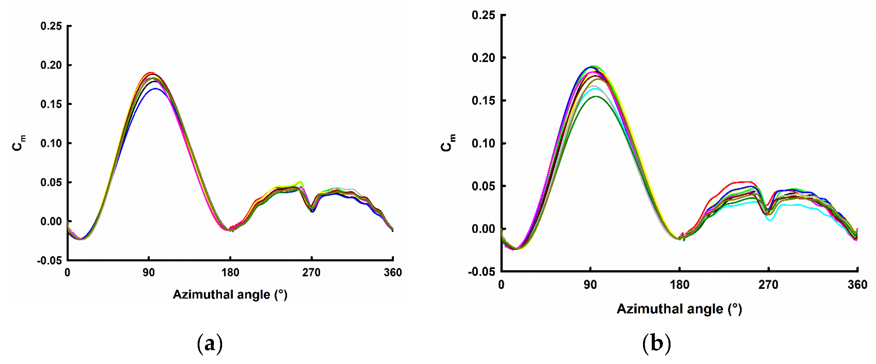
• The effect of inlet velocities randomisation parameters such as input randomised fluctuation of 6 m/s, 4 m/s, and 2 m/s were investigated. The average C_p value and magnitude of fluctuation of velocity was higher, with an increase in the magnitude of randomised fluctuation.
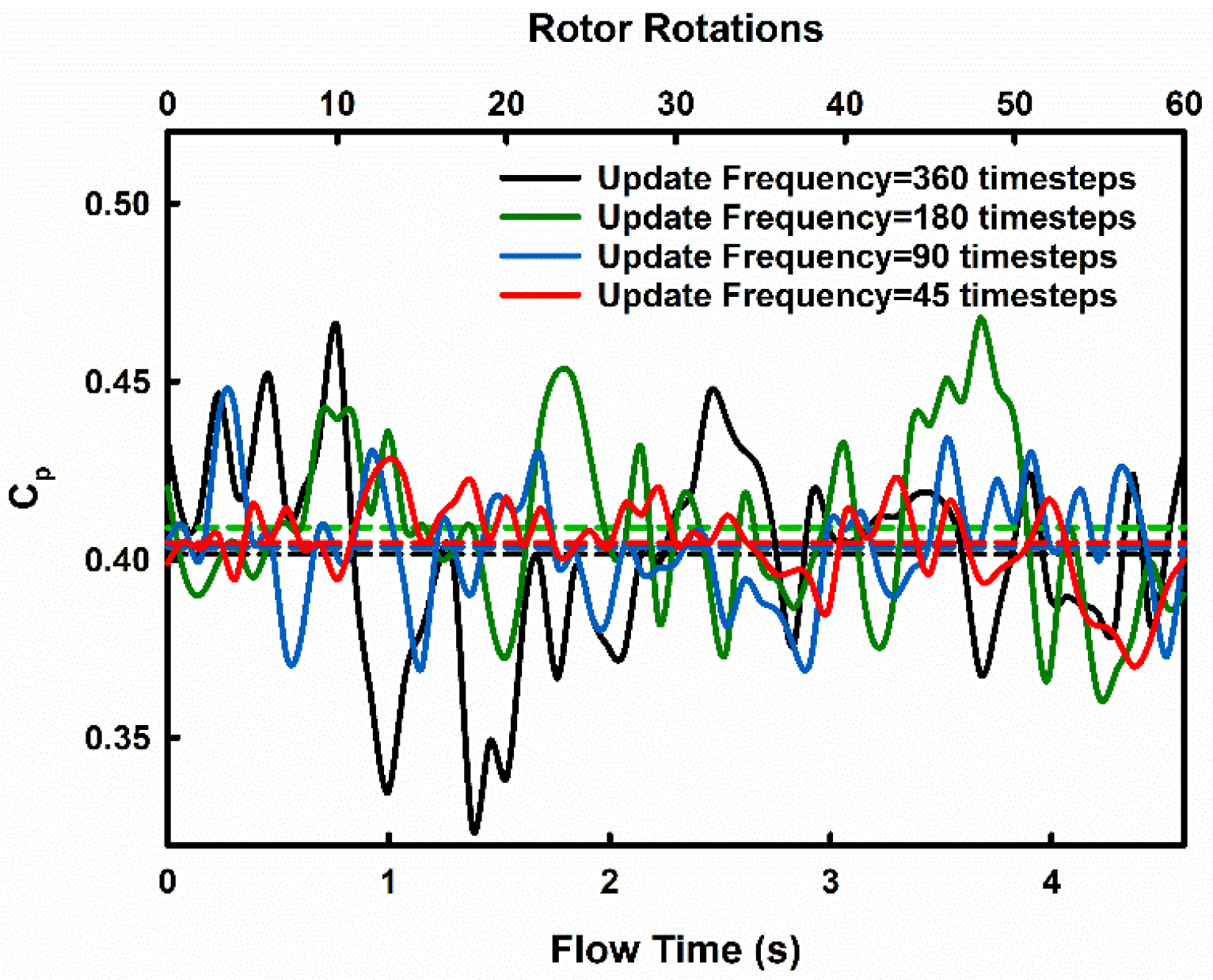
• The effect of randomisation update frequencies of 45, 90,180, and 360 time-steps was also studied. There was a decrease in the magnitude of velocity fluctuations from the update frequency 360 time-steps to the update frequency of 45 time-steps. The flow field upstream of the turbine was more uniform for the update frequency of 45 time-steps than for the update frequency of 360 time-steps, which is characterised by a higher magnitude of macro-turbulence. As the update interval decreases, the flow field in front of the turbine becomes uniform. The magnitude of C_p fluctuations also decreases with the size of the update interval.
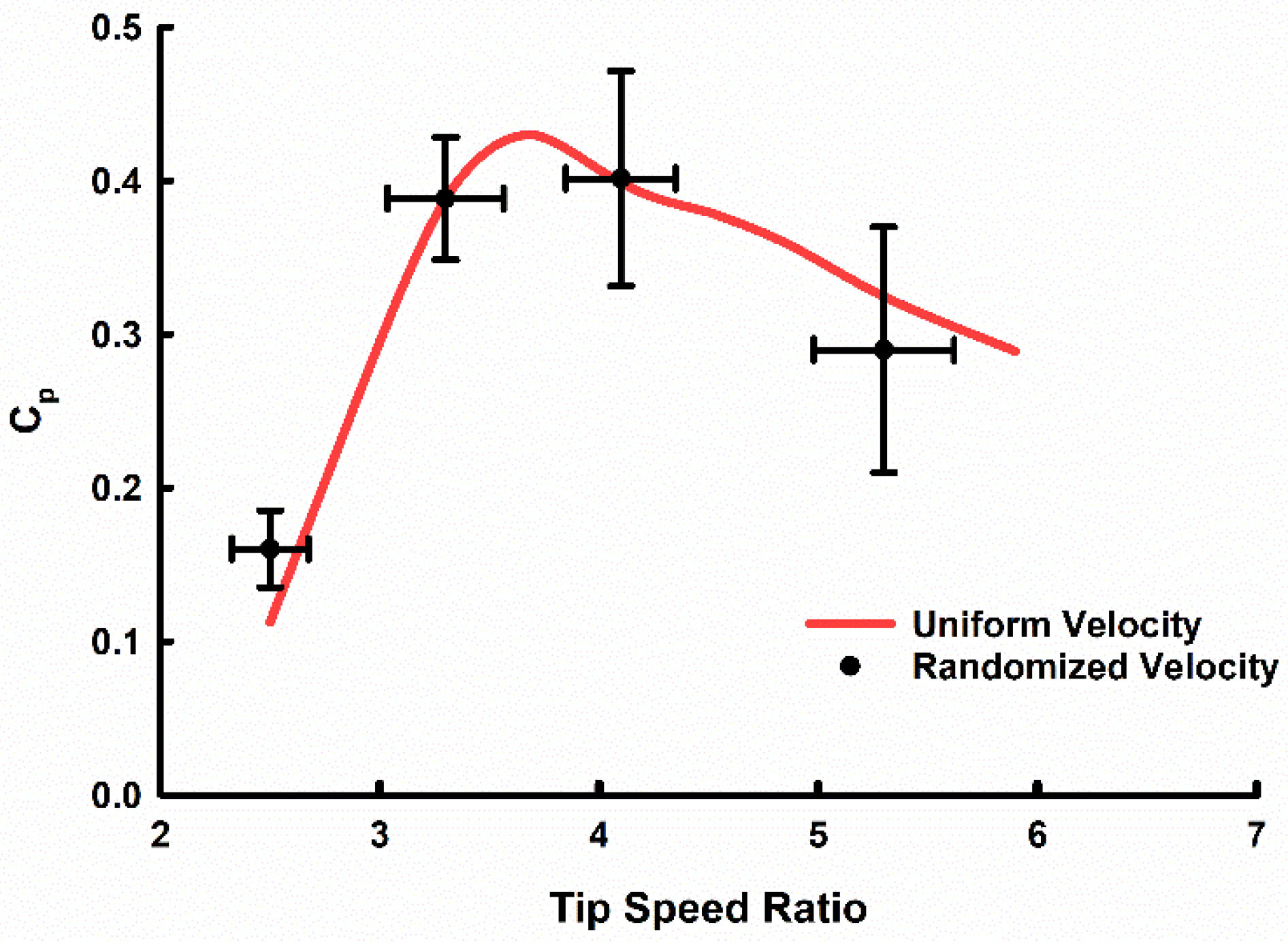
• The effect of the tip speed ratio on a wind turbine for randomised inlet conditions was also studied. The magnitude of fluctuation of velocity also decreased with an increase in tip speed ratio. Though randomised and uniform flow follows the same C_p-λ trend, the slope was steeper for randomised, and there was a visible difference in the C_p values at λ = 2.5 and λ = 5.3. The performance of the VAWT was highly sensitive at higher tip speed ratios. Thus, the operational range of tip speed ratio to extract maximum power from available wind should be around 4.1 for a 2 bladed turbine of 1 m diameter and solidity of 0.12.
• The variation of C_m given for a single blade for a rotor rotation for various tip speed ratios was also studied. It was noticed that at lower tip speed ratios, the peak C_m occurred before 90° and a drop in moment coefficient to negative values after dynamic stall was observed. During downstream conditions, vortex shedding from the central shaft contributed to higher moment coefficient values and larger variations for λ = 2.5 compared to other tip speed ratios.
• The effect of tip speed ratio on the turbine wake recovery was also studied. As the tip speed ratio increased, the velocity deficit in the wake structure also increased. Streamwise velocity behind the turbine was highly reduced. For near wake cases, x/d = 2.5 and x/d = 4, the velocity deficit values were comparable for all tip speed ratios. As the downstream distance increased, the velocity deficit decreased for all tip speed ratios. Wake recovery was faster in the case of lower tip speed ratios. Wake generated by uniform velocity inlet had slower wake recovery compared to randomised velocity inlet. Macro-turbulence generated by randomisation enhanced the mixing of flow downwind of the turbine, allowing faster recovery.
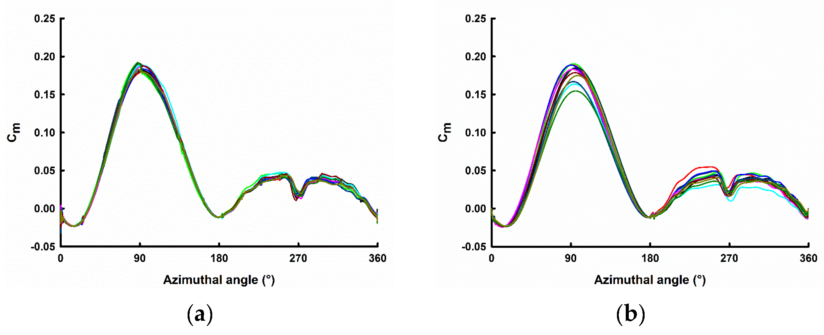
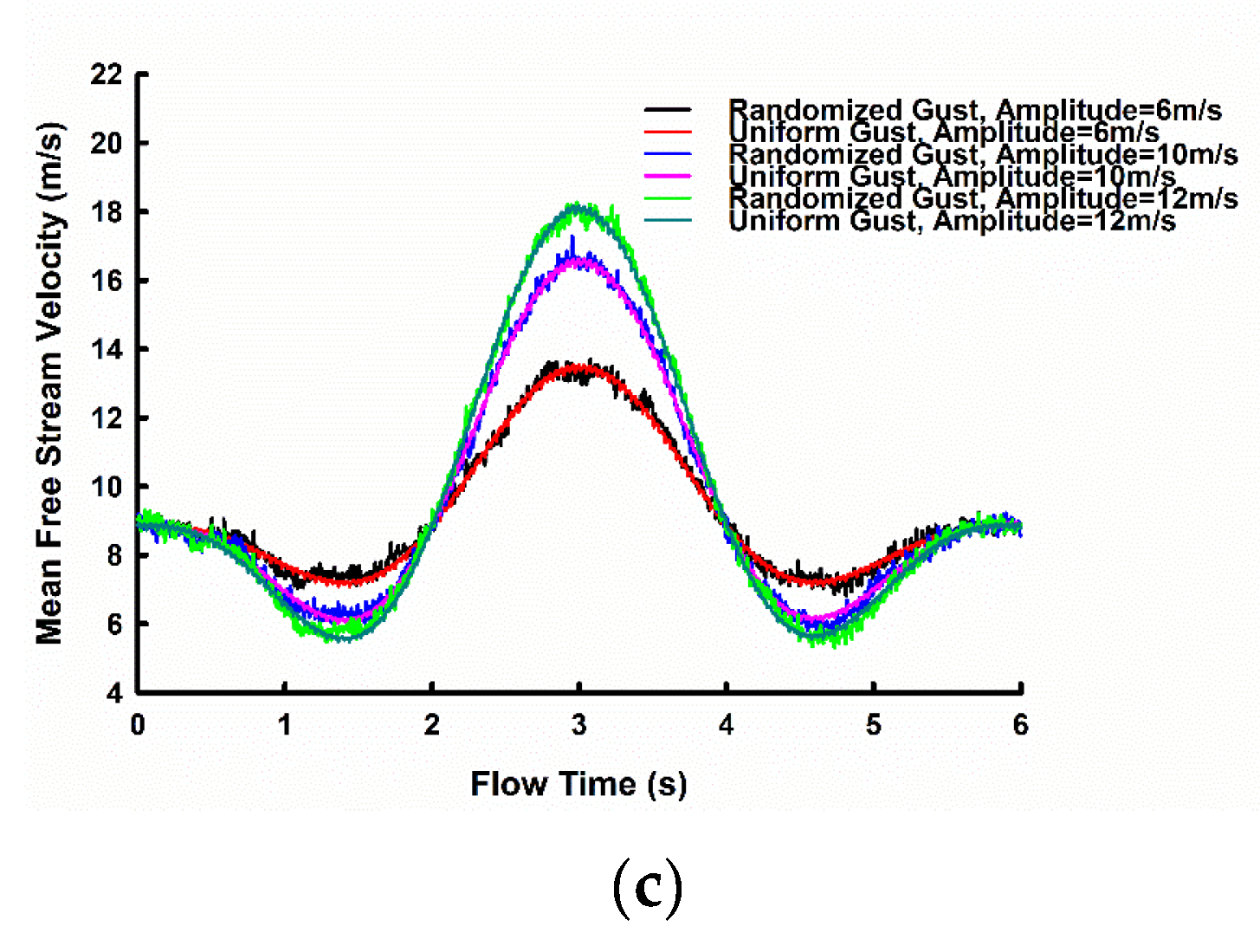
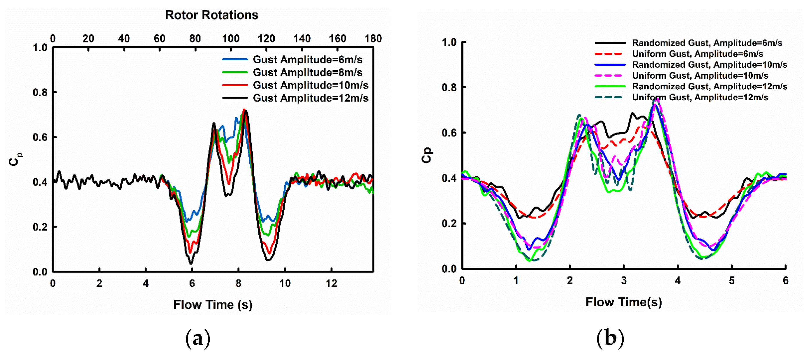
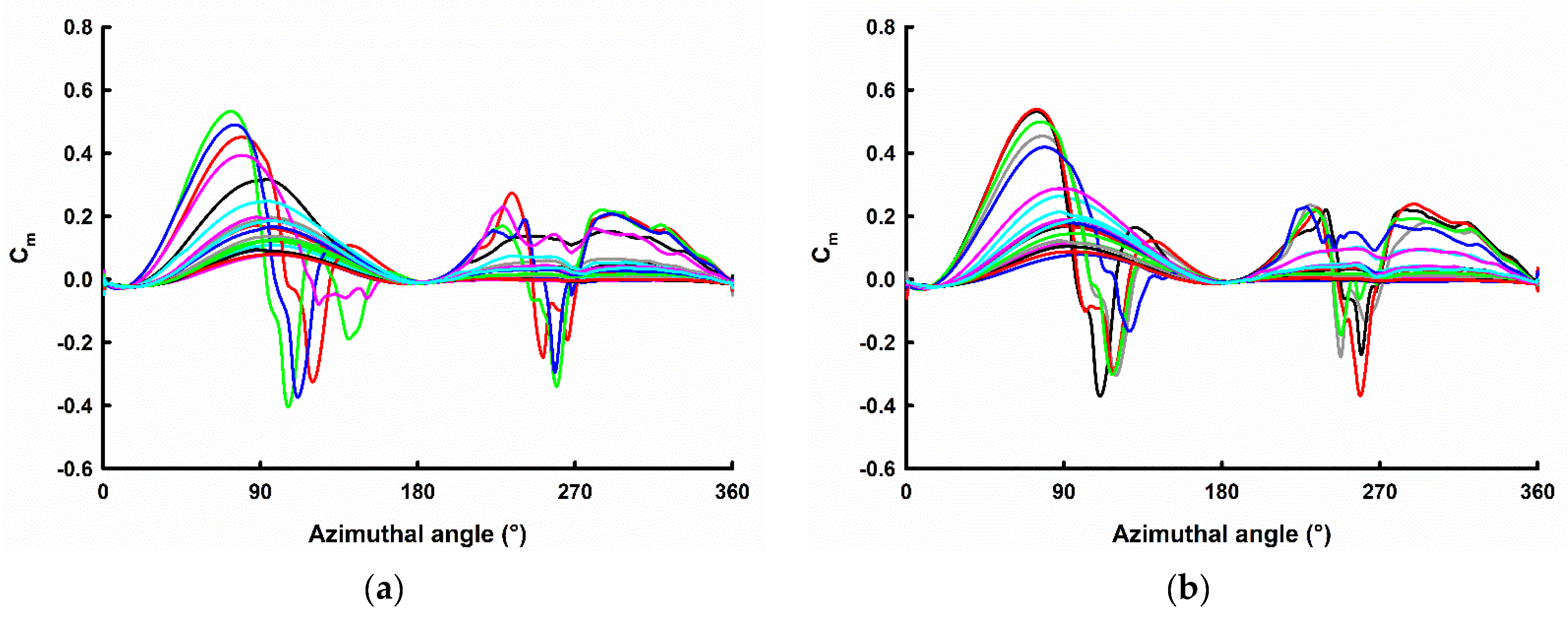
• Further, a study was performed on the influence of gust parameters such as gust amplitude and gust time period on the coefficient of power of the VAWT, for an IEC extreme operating gust. Since the average gust factor is 1.44 in extreme cases, 4 different randomised cases of U_gust = 6 m/s, 8 m/s, 10 m/s, and 12 m/s with gust factors of 1.34, 1.50, 1.64, and 1.80, respectively, were considered. A comparison of U_∞ for uniform gust cases and randomised gust cases showed that the spatial fluctuation in the velocity profile of randomised gust subsequently affected the C_p values of the wind turbine. The tip speed ratio vs. flow time plots also showed fluctuations for all gust cases. Unlike the case with a steady inlet velocity of 10 m/s, the C_m vs. azimuthal angle for U_gust deviated from the general profile due to continuously varying tip speed ratios. The deviation occurred for turbine cycles where free stream velocity was greater than 14 m/s, i.e., the tip speed ratio was less than 2.92. This was clearly observed in gust cases with higher gust magnitude, U_gust = 10 m/s and U_gust = 12 m/s. As tip speed ratios increased, cycles had a lower value of peak C_m during the upwind condition and C_m values were not negative.
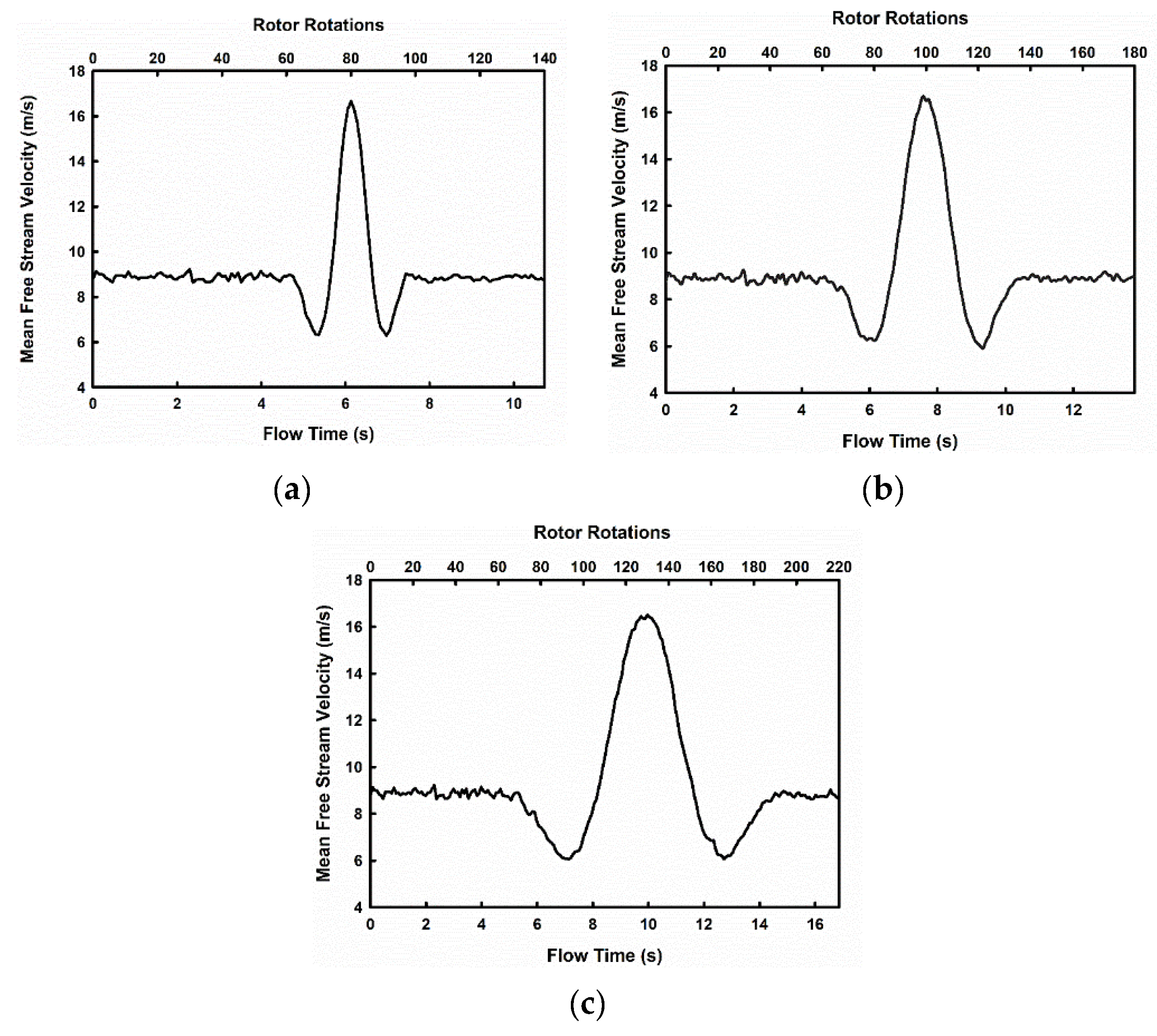
• The effect of time period was investigated for U_gust = 10 m/s, and gust factor 1.64 was studied for gust time periods T = 3 s, 6 s, 10.5 s. All cases showed similar values of maximum and minimum velocities and tip speed ratios, spread over the respective time periods. The C_p plot for 10.5 s gust showed many fluctuations in the region where velocity rises to the maximum.

References

1. Kusch-Brandt, S. Renewables 2019 Global Status Report. 2019, Volume 8. 9783981891140. Available online: https://www.ren21.net/wp-content/uploads/2019/05/2018-2019-Annual-Report_FINAL_low-res.pdf (accessed on 12 January 2023).
2. Emejeamara, F.C.; Tomlin, A.S.; Millward-Hopkins, J.T. Urban wind: Characterisation of useful gust and energy capture. Renew. Energy 2015, 81, 162–172. [Google Scholar] [CrossRef] [Green Version]
3. Johari, M.K.; Jalil, M.A.A.; Shariff, M.F.M. Comparison of horizontal axis wind turbine (HAWT) and vertical axis wind turbine (VAWT). Int. J. Eng. Technol. 2018, 7, 74–80. [Google Scholar] [CrossRef] [Green Version]
4. Pagnini, L.C.; Burlando, M.; Repetto, M.P. Experimental power curve of small-size wind turbines in turbulent urban environment. Appl. Energy 2015, 154, 112–121. [Google Scholar] [CrossRef]
5. Toja-Silva, F.; Colmenar-Santos, A.; Castro-Gil, M. Urban wind energy exploitation systems: Behaviour under multidirectional flow conditions—Opportunities and challenges. Renew. Sustain. Energy Rev. 2013, 24, 364–378. [Google Scholar] [CrossRef]
6. Ishugah, T.F.; Li, Y.; Wang, R.Z.; Kiplagat, J.K. Advances in wind energy resource exploitation in urban environment: A review. Renew. Sustain. Energy Rev. 2014, 37, 613–626. [Google Scholar] [CrossRef]
7. Tummala, A.; Velamati, R.K.R.K.; Sinha, D.K.; Indraja, V.; Krishna, V.H.; Subramanian, A.; Yogesh, S.A.; Sivanandan, H.; Giri, A.; Vasudevan, M.; et al. Progress and recent trends of wind energy technology. Renew. Sustain. Energy Rev. 2013, 21, 456–468. [Google Scholar] [CrossRef]
8. Britter, R.E.; Hanna, S.R. Flow and dispersion in urban areas. Annu. Rev. Fluid Mech. 2003, 35, 469–496. [Google Scholar] [CrossRef]
9. Mantravadi, B.; Unnikrishnan, D.; Sriram, K.; Mohammad, A.; Vaitla, L.; Velamati, R.K. Effect of solidity and airfoil on the performance of vertical axis wind turbine under fluctuating wind conditions. Int. J. Green Energy 2019, 16, 1329–1342. [Google Scholar] [CrossRef]
10. Tavernier, D.D.; Ferreira, C. The need for dynamic inflow models for vertical axis wind turbines. J. Phys. Conf. Ser. 2019, 1356. [Google Scholar] [CrossRef] [Green Version]
11. McIntosh, S.C.; Babinsky, H.; Bertényi, T. Optimizing the energy output of vertical axis wind turbines for fluctuating wind conditions. In Proceedings of the Collect Tech Pap—45th AIAA Aerospace Sciences Meeting, Reno, NV, USA, 8–11 January 2007; Volume 23, pp. 16202–16214. [Google Scholar] [CrossRef]
12. Wekesa, D.W.; Wang, C.; Wei, Y.; Danao, L.A.M. Analytical and numerical investigation of unsteady wind for enhanced energy capture in a fluctuating free-stream. Energy 2017, 121, 854–864. [Google Scholar] [CrossRef]
13. Battisti, L.; Benini, E.; Brighenti, A.; Soraperra, G.; Castelli, M.R. Simulating the dynamic behavior of a vertical axis wind turbine operating in unsteady conditions. J. Phys. Conf. Ser. 2016, 753. [Google Scholar] [CrossRef]
14. Bhargav, M.; Kishore, V.R.; Laxman, V. Influence of fluctuating wind conditions on vertical axis wind turbine using a three dimensional CFD model. J. Wind Eng. Ind. Aerodyn. 2016, 158, 98–108. [Google Scholar] [CrossRef]
15. Wekesa, D.W.; Wang, C.; Wei, Y.; Kamau, J.N.; Danao, L.A.M. A numerical analysis of unsteady inflow wind for site specific vertical axis wind turbine: A case study for Marsabit and Garissa in Kenya. Renew. Energy 2015, 76, 648–661. [Google Scholar] [CrossRef]
16. Bausas, M.D.; Danao, L.A.M. The aerodynamics of a camber-bladed vertical axis wind turbine in unsteady wind. Energy 2015, 93, 1155–1164. [Google Scholar] [CrossRef]
17. Danao, L.A.; Edwards, J.; Eboibi, O.; Howell, R. A numerical investigation into the influence of unsteady wind on the performance and aerodynamics of a vertical axis wind turbine. Appl. Energy 2014, 116, 111–124. [Google Scholar] [CrossRef] [Green Version]
18. Danao, L.A.; Eboibi, O.; Howell, R. An experimental investigation into the influence of unsteady wind on the performance of a vertical axis wind turbine. Appl. Energy 2013, 107, 403–411. [Google Scholar] [CrossRef]
19. Scheurich, F.; Brown, R.E. Modelling the aerodynamics of vertical-axis wind turbines in unsteady wind conditions. Wind Energy 2013, 16, 91–107. [Google Scholar] [CrossRef] [Green Version]
20. Wu, Z.; Wang, Q.; Bangga, G.; Huang, H. Responses of vertical axis wind turbines to gusty winds. Proc. Inst. Mech. Eng. Part A J. Power Energy 2020, 235, 81–93. [Google Scholar] [CrossRef]
21. Wu, Z.; Bangga, G.; Cao, Y. Effects of lateral wind gusts on vertical axis wind turbines. Energy 2019, 167, 1212–1223. [Google Scholar] [CrossRef]
22. Rakib, M.I.; Evans, S.P.; Clausen, P.D. Measured gust events in the urban environment, a comparison with the IEC standard. Renew. Energy 2020, 146, 1134–1142. [Google Scholar] [CrossRef]
23. Onol, A.O.; Yesilyurt, S. Effects of wind gusts on a vertical axis wind turbine with high solidity. J. Wind Eng. Ind. Aerodyn. 2017, 162, 1–11. [Google Scholar] [CrossRef]
24. Kwon, D.K.; Kareem, A.; Butler, K. Gust-front loading effects on wind turbine tower systems. J. Wind Eng. Ind. Aerodyn. 2012, 104–106, 109–115. [Google Scholar] [CrossRef]
25. Cheng, P.W.; Bierbooms, W.A.A.M. Distribution of extreme gust loads of wind turbines. J. Wind Eng. Ind. Aerodyn. 2001, 89, 309–324. [Google Scholar] [CrossRef]
26. Bierbooms, W.; Cheng, P.W. Modelling of Extreme Gusts for Design Calculations. In Proceedings of the EUWEC 96, Göteborg, Sweden, 20–24 May 2000; pp. 842–845. [Google Scholar]
27. Balduzzi, F.; Zini, M.; Ferrara, G.; Bianchini, A. Development of a computational fluid dynamics methodology to reproduce the effects of macroturbulence on wind turbines and its application to the particular case of a VAWT. J. Eng. Gas Turbines Power 2019, 141, 1–12. [Google Scholar] [CrossRef]
28. KC, A.; Whale, J.; Urmee, T. Urban wind conditions and small wind turbines in the built environment: A review. Renew. Energy 2019, 131, 268–283. [Google Scholar] [CrossRef]
29. Shahzad, A.; Asim, T.; Mishra, R.; Paris, A. Performance of a vertical axis wind turbine under accelerating and decelerating flows. Procedia CIRP 2013, 11, 311–316. [Google Scholar] [CrossRef] [Green Version]
30. Jafari, M.; Razavi, A.; Mirhosseini, M. Effect of Steady and Quasi-Unsteady Wind on Aerodynamic Performance of H-Rotor Vertical Axis Wind Turbines. J. Energy Eng. 2018, 144, 04018065. [Google Scholar] [CrossRef]
31. Lee, K.Y.; Tsao, S.H.; Tzeng, C.W.; Lin, H.J. Influence of the vertical wind and wind direction on the power output of a small vertical-axis wind turbine installed on the rooftop of a building. Appl. Energy 2018, 209, 383–391. [Google Scholar] [CrossRef]
32. IEC Standard 61400-2; International Standard—Part 2: Small Wind Turbines. International Electrotechnical Commission: London, UK, 2006; Volume 2006, ISBN 2831886376.
33. Stork, C.H.J.; Butterfield, C.P.; Holley, W.; Madsen, P.H.; Jensen, P.H. Wind conditions for wind turbine design proposals for revision of the IEC 1400-1 standard. J. Wind Eng. Ind. Aerodyn. 1998, 74–76, 443–454. [Google Scholar] [CrossRef]
34. Lam, H.F.; Peng, H.Y. Study of wake characteristics of a vertical axis wind turbine by two- and three-dimensional computational fluid dynamics simulations. Renew. Energy 2016, 90, 386–398. [Google Scholar] [CrossRef]
35. Peng, H.Y.; Lam, H.F.; Lee, C.F. Investigation into the wake aerodynamics of a five-straight-bladed vertical axis wind turbine by wind tunnel tests. J. Wind Eng. Ind. Aerodyn. 2016, 155, 23–35. [Google Scholar] [CrossRef]
36. Rezaeiha, A.; Montazeri, H.; Blocken, B. Characterization of aerodynamic performance of vertical axis wind turbines: Impact of operational parameters. Energy Convers. Manag. 2018, 169, 45–77. [Google Scholar] [CrossRef]
37. Daróczy, L.; Janiga, G.; Petrasch, K.; Webner, M.; Thévenin, D. Comparative analysis of turbulence models for the aerodynamic simulation of H-Darrieus rotors. Energy 2015, 1–11. [Google Scholar] [CrossRef]
38. Rezaeiha, A.; Montazeri, H.; Blocken, B. On the accuracy of turbulence models for CFD simulations of vertical axis wind turbines. Energy 2019, 180, 838–857. [Google Scholar] [CrossRef]
39. Rezaeiha, A.; Kalkman, I.; Blocken, B. CFD simulation of a vertical axis wind turbine operating at a moderate tip speed ratio: Guidelines for minimum domain size and azimuthal increment. Renew. Energy 2017, 107, 373–385. [Google Scholar] [CrossRef] [Green Version]
40. Bianchini, A.; Balduzzi, F.; Bachant, P.; Ferrara, G.; Ferrari, L. Effectiveness of two-dimensional CFD simulations for Darrieus VAWTs: A combined numerical and experimental assessment. Energy Convers. Manag. 2017, 136, 318–328. [Google Scholar] [CrossRef]
41. Castelli, M.R.; Englaro, A.; Benini, E. The Darrieus wind turbine: Proposal for a new performance prediction model based on CFD. Energy 2011, 36, 4919–4934. [Google Scholar] [CrossRef]
Figure 1. (a) Velocity contour of non-uniform flow upstream of the VAWT; (b) Temporal variation of average free stream wind velocity upstream of the VAWT.
Energies 16 02250 g001
Figure 2. (a) Computational domain ABCD; (b) A representation of straight-bladed VAWT with 3 blades.
Energies 16 02250 g002
Figure 3. Details of computational grid used in the present work. (a) Overall grid of the entire domain; (b) Mesh in the rotation part of domain (c) grid around the wind turbine blade.
Energies 16 02250 g003
Figure 4. Validation of numerical model with experimental results [36,41] and other standard numerical results.
Energies 16 02250 g004
Figure 5. Grid independence study conducted using three different grid numbers.
Energies 16 02250 g005
Figure 6. (a) Variation of Cp for various randomised fluctuation; the mean and minimum maximum is represented in the graph with the help of dashed lines and dotted lines respectively; (b) Effect of free stream velocity on Cp.
Energies 16 02250 g006
Figure 7. Moment coefficient for various rotational cycles. (a) Randomised Fluctuation = 2 m/s; (b) Randomised Fluctuation = 6 m/s. Coefficient of Moment at various time instances (rotational cycles) are represented through different coloured lines. Due to randomized wind conditions, values vary every rotational cycle.
Energies 16 02250 g007
Figure 8. (a) Effect of update frequency on the average wind velocity upstream of VAWT; (b) Snapshots of flow field upstream of VAWT for Randomisation Update Frequency = 360 time-steps; (c) Snapshots of flow field upstream of VAWT for Randomisation Update Frequency = 45 time-steps.
Energies 16 02250 g008aEnergies 16 02250 g008b
Figure 9. Variation of Cp for various randomisation update frequencies. Corresponding mean Cp is represented through dashed lines.
Energies 16 02250 g009
Figure 10. Coefficient of Moment (Cm) for various rotational cycles. (a) Randomisation Update Frequency = 45 time-steps; (b) Randomisation Update Frequency = 360 time-steps. Coefficient of Moment at various time instances (rotational cycles) are represented through different coloured lines. Due to randomized wind conditions, values vary every rotational cycle.
Energies 16 02250 g010
Figure 11. Effect of tip speed ratio on the average wind velocity upstream of VAWT. (a) 0.75 d; (b) 1 d; (c) 1.25 d. The mean and minimum-maximum is represented in the graph with the help of dashed lines and dotted lines respectively.
Energies 16 02250 g011aEnergies 16 02250 g011b
Figure 12. Effect of tip speed ratio on Coefficient of Performance (Cp) with random wind conditions.
Energies 16 02250 g012
Figure 13. Coefficient of Moment (Cm) for various rotational cycles. (a) λ = 2.5; (b) λ = 3.3; (c) λ = 4.1; (d) λ = 5.3. Coefficient of Moment at various time instances (rotational cycles) are represented through different coloured lines. Due to randomized wind conditions, values vary every rotational cycle.
Energies 16 02250 g013
Figure 14. Time-averaged normalised stream-wise wake velocity along −0.75 d ≤ y/d ≤ +0.75 d for different tip speed ratios at near-wake distances. (a) x/d = 2.5; (b) x/d = 4. Instantaneous normalised stream-wise wake velocity profiles are represented using dotted lines.
Energies 16 02250 g014
Figure 15. Time averaged normalised stream-wise wake velocity along −0.75 d ≤ y/d ≤ +0.75 d for different tip speed ratios at near-wake distances. (a) x/d = 6; (b) x/d = 8; (c) x/d = 10. Instantaneous normalised stream-wise wake velocity profiles are represented using dotted lines.
Energies 16 02250 g015
Figure 16. Time averaged normalised stream-wise wake velocity along −0.75 d ≤ y/d ≤ +0.75 d for all wake distances for (a) λ = 2.5; (b) λ = 5.3.
Energies 16 02250 g016
Figure 17. (a) The variation in cycle-averaged U∞ for Ugust = 6 m/s, 8 m/s, 10 m/s and 12 m/s; (b) Instantaneous variation of U∞ for Ugust = 6 m/s, 8 m/s, 10 m/s and 12 m/s; (c) Comparison of Randomised Gust velocity and Uniform gust velocity.
Energies 16 02250 g017aEnergies 16 02250 g017b
Figure 18. (a) The variation in cycle-averaged tip speed ratio for Ugust = 6 m/s, 8 m/s, 10 m/s, and 12 m/s; (b) Instantaneous variation of tip speed ratio for Ugust = 6 m/s, 8 m/s, 10 m/s and 12 m/s.
Energies 16 02250 g018
Figure 19. Variation of Coefficient of Moment Cm for azimuthal Angle for (a) Ugust = 6 m/s; (b) Ugust = 8 m/s; (c) Ugust = 10 m/s; (d) Ugust = 12 m/s. Coefficient of Moment at various time instances (rotational cycles) are represented through different coloured lines. Due to randomized wind conditions, values vary every rotational cycle.
Energies 16 02250 g019aEnergies 16 02250 g019b
Figure 20. (a) Variation of Cp for flow time for Ugust = 6 m/s, 8 m/s, 10 m/s, and 12 m/s; (b) Comparison of Cp of randomised gust velocity case with uniform gust velocity case against flow time.
Energies 16 02250 g020
Figure 21. The variation of cycle-averaged mean free stream velocity (U∞) for gust time periods (a) 3 s; (b) 6 s; (c) 10.5 s.
Energies 16 02250 g021
Figure 22. The variation of tip speed ratio (λ) for gust time periods (a) 3 s; (b) 6 s; (c) 10.5 s.
Energies 16 02250 g022
Figure 23. The variation of Cp for flow time for one complete gust cycle gust time periods (a) 3 s; (b) 6 s; (c) 10.5 s.
Energies 16 02250 g023aEnergies 16 02250 g023b
Figure 24. Variation of Coefficient of Moment (Cm) with azimuthal angle for gust time periods (a) 3 s; (b) 10.5 s. Coefficient of Moment at various time instances (rotational cycles) are represented through different coloured lines. Due to randomized wind conditions, values vary every rotational cycle.
Energies 16 02250 g024